World-set Decompositions:
Expressiveness and Efficient Algorithms

Abstract

Uncertain information is commonplace in real-world data management scenarios. The ability to represent large sets of possible instances (worlds) while supporting efficient storage and processing is an important challenge in this context. The recent formalism of world-set decompositions (WSDs) provides a space-efficient representation for uncertain data that also supports scalable processing. WSDs are complete for finite world-sets in that they can represent any finite set of possible worlds. For possibly infinite world-sets, we show that a natural generalization of WSDs precisely captures the expressive power of c-tables. We then show that several important problems are efficiently solvable on WSDs while they are NP-hard on c-tables. Finally, we give a polynomial-time algorithm for factorizing WSDs, i.e. an efficient algorithm for minimizing such representations.

1 Introduction

Recently there has been renewed interest in incomplete information databases. This is due to the many important applications that systems for representing incomplete information have, such as data cleaning, data integration, and scientific databases.

Strong representation systems [19, 3, 18] are formalisms for representing sets of possible worlds which are closed under query operations in a given query language. While there have been numerous other approaches to dealing with incomplete information, such as closing possible worlds semantics using certain answers [1, 7, 12], constraint or database repair [13, 10, 9], and probabilistic ranked retrieval [14, 4], strong representation systems form a compositional framework that is minimally intrusive by not requiring to lose information, even about the lack of information, present in an information system: Computing certain answers, for example, entails a loss of possible but uncertain information. Strong representation systems can be nicely combined with the other approaches. For example, data transformation queries and data cleaning steps effected within a strong representation systems framework can be followed by a query with ranked retrieval or certain answers semantics, closing the possible worlds semantics.

The so-called c-tables [19, 16, 17] are the prototypical strong representation system. However, c-tables are not well suited for representing large incomplete databases in practice. Two recent works presented strong, indeed complete, representation systems for finite sets of possible worlds. The approach of the Trio x-relations [8] relies on a form of intensional information (“lineage”) only in combination with which the formalism is strong. In [5] large sets of possible worlds are managed using world-set decompositions (WSDs). The approach is based on relational product decomposition to permit space-efficient representation. [5] describes a prototype implementation and shows the efficiency and scalability of the formalism in terms of storage and query evaluation in a large census data scenario with up to $2^{10^{6}}$ worlds, where each world stored is several GB in size.

Examples of world-set decompositions.

As WSDs play a central role in this work, we next exemplify them using two manually completed forms that may originate from a census and which allow for more than one interpretation (Figure 1). For simplicity we assume that social security numbers consist of only three digits. For instance, Smith’s social security number can be read either as “185” or as “785”. We can represent the available information using a relation in which possible alternative values are represented in set notation (so-called or-sets):

(TID)	S	N	M
$t_{1}$	{ 185, 785 }	Smith	{ 1, 2 }
$t_{2}$	{ 185, 186 }	Brown	{ 1, 2, 3, 4 }

This or-set relation represents $2\cdot 2\cdot 2\cdot 4=32$ possible worlds.

We now enforce the integrity constraint that all social security numbers be unique. For our example database, this constraint excludes 8 of the 32 worlds, namely those in which both tuples have the value 185 as social security number. This constraint excludes the worlds in which both tuples have the value 185 as social security number. It is impossible to represent the remaining 24 worlds using or-set relations. What we could do is store each world explicitly using a table called a world-set relation of a given set of worlds. Each tuple in this table represents one world and is the concatenation of all tuples in that world (see Figure 1).

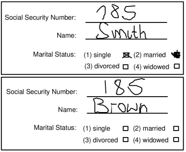
$t_{1}.S$	$t_{1}.N$	$t_{1}.M$	$t_{2}.S$	$t_{2}.N$	$t_{2}.M$
185	Smith	1	186	Brown	1
185	Smith	1	186	Brown	2
185	Smith	1	186	Brown	3
185	Smith	1	186	Brown	4
185	Smith	2	186	Brown	1
185	Smith	2	186	Brown	2
185	Smith	2	186	Brown	3
185	Smith	2	186	Brown	4
⋮
785	Smith	2	186	Brown	4

Figure 1: Two completed survey forms and a world-set relation representing the possible worlds with unique social security numbers.

A world-set decomposition is a decomposition of a world-set relation into several relations such that their product (using the product operation of relational algebra) is again the world-set relation. The world-set represented by our initial or-set relation can also be represented by the product

185785×t1.NSmith× 12× 185186×t2.NBrown× 1234 fragments185785fragmentst1.NSmith 12 185186fragmentst2.NBrown 1234\begin{tabular}[]{|c|}\hline\cr$t_{1}.S$\\ \hline\cr 185\\ 785\\ \hline\cr\end{tabular}\times\begin{tabular}[]{|c|}\hline\cr$t_{1}.N$\\ \hline\cr Smith\\ \hline\cr\end{tabular}\times\begin{tabular}[]{|c|}\hline\cr$t_{1}.M$\\ \hline\cr 1\\ 2\\ \hline\cr\end{tabular}\times\begin{tabular}[]{|c|}\hline\cr$t_{2}.S$\\ \hline\cr 185\\ 186\\ \hline\cr\end{tabular}\times\begin{tabular}[]{|c|}\hline\cr$t_{2}.N$\\ \hline\cr Brown\\ \hline\cr\end{tabular}\times\begin{tabular}[]{|c|}\hline\cr$t_{2}.M$\\ \hline\cr 1\\ 2\\ 3\\ 4\\ \hline\cr\end{tabular}

$$\begin{array}{c}\end{array}$$t1.St1.Mt2.St2.Mt1.St1.Mt2.St2.M

In the same way we can represent the result of data cleaning with the uniqueness constraint for the social security numbers as the product

185186785185785186×t1.NSmith× 12×t2.NBrown× 1234fragments 185186785185785186fragmentst1.NSmith 12fragmentst2.NBrown 1234\begin{tabular}[]{|c@{\extracolsep{1mm}}c|}\hline\cr$t_{1}.S$&$t_{2}.S$\\ \hline\cr 185&186\\ 785&185\\ 785&186\\ \hline\cr\end{tabular}\times\begin{tabular}[]{|c|}\hline\cr$t_{1}.N$\\ \hline\cr Smith\\ \hline\cr\end{tabular}\times\begin{tabular}[]{|c|}\hline\cr$t_{1}.M$\\ \hline\cr 1\\ 2\\ \hline\cr\end{tabular}\times\begin{tabular}[]{|c|}\hline\cr$t_{2}.N$\\ \hline\cr Brown\\ \hline\cr\end{tabular}\times\begin{tabular}[]{|c|}\hline\cr$t_{2}.M$\\ \hline\cr 1\\ 2\\ 3\\ 4\\ \hline\cr\end{tabular}

t1.St2.St1.Mt2.Mt1.St2.St1.Mt2.M

One can observe that the result of this product is exactly the world-set relation in Figure 1. The decomposition is based on the independence between sets of fields, subsequently called components. Only fields that depend on each other, for example $t_{1}.S$ and $t_{2}.S$, belong to the same component. Since $\{t_{1}.S,t_{2}.S\}$ and $\{t_{1}.M\}$ are independent, they are put into different components.

WSDs can be naturally viewed as c-tables whose formulas have been put into a normal form represented by the component relations. The following c-table with global condition $\phi$ is equivalent to the WSD with our integrity constraint enforced.

T	S	N	M	cond
				$\phi=((x=185\land z=186)\lor(x=785\land z=185)\lor$
				$(x=785\land z=186))\land(y=1\lor y=2)\land$
				$(w=1\lor w=2\lor w=3\lor w=4)$
	$x$	Smith	$y$
	$z$	Brown	$w$

Formal definitions of WSDs and c-tables will be given in the body of this article.

Contributions.

Input Representation system ${\cal W}$, instance $I=(R^{I})$, tuple $t$ Problems Tuple possibility: $\exists{\cal A}\in\mathit{rep}({\cal W}):t\in R^{\cal A}$ Tuple certainty: $\forall{\cal A}\in\mathit{rep}({\cal W}):t\in R^{\cal A}$ Instance possibility: $\exists{\cal A}\in\mathit{rep}({\cal W}):R^{I}=R^{\cal A}$ Instance certainty: $\forall{\cal A}\in\mathit{rep}({\cal W}):R^{I}=R^{\cal A}$ Tuple q-possibility (query q fixed): $\exists{\cal A}\in\mathit{rep}({\cal W}):t\in q({\cal A})$ Tuple q-certainty (query q fixed): $\forall{\cal A}\in\mathit{rep}({\cal W}):t\in q({\cal A})$ Instance q-possibility (query q fixed): $\exists{\cal A}\in\mathit{rep}({\cal W}):R^{I}=q({\cal A})$ Instance q-certainty (query q fixed): $\forall{\cal A}\in\mathit{rep}({\cal W}):R^{I}=q({\cal A})$

Table 1: Decision Problems for Representation Systems.

The main goal of this work is to develop expressive yet efficient representation systems for infinite world-sets and to study the theoretical properties (such as expressive power, complexity of query-processing, and minimization) of these representation systems. Many of these results also apply to – and are new for – the world-set decompositions of [5].

In [18], a strong argument is made supporting c-tables as a benchmark for the expressiveness of representation systems; we concur. Concerning efficient processing, we adopt a less expressive syntactic restriction of c-tables, called v-tables [19, 3], as a lower bound regarding succinctness and complexity. The main development of this article is a representation system that combines, in a sense, the best of all worlds: (1) It is just as expressive as c-tables, (2) it is exponentially more succinct than unions of v-tables, and (3) on most classical decision problems, the complexity bounds are not worse than those for v-tables.

In more detail, the technical contributions of this article are as follows:

• We introduce gWSDs, an extension of the WSD model of [5] with variables and possibly negated equality conditions.

• We show that gWSDs are expressively equivalent to c-tables and are therefore a strong representation system for full relational algebra.

• We study the complexity of the main data management problems [3, 19] regarding WSDs and gWSDs, summarized in Table 1. Table 2 compares the complexities of these problems in our context to those of existing strong representation systems like the well-behaved ULDBs of Trio and c-tables.

• We present an efficient algorithm for optimizing gWSDs, i.e., for computing an equivalent gWSD whose size is smaller than that of a given gWSD. In the case of WSDs, this is a minimization algorithm that produces the unique maximal decomposition of a given WSD.

	v-tables [3]	(g)WSDs	Trio [8]	c-tables [17]
Tuple possibility	PTIME	PTIME	PTIME	NP-compl.
Tuple certainty	PTIME	PTIME	PTIME	coNP-compl.
Instance possibility	NP-compl.	NP-compl.	NP-hard	NP-compl.
Instance certainty	PTIME	PTIME	NP-hard	coNP-compl.
Tuple q-possibility	NP-compl.	NP-compl.	?	NP-compl.
positive relational algebra	PTIME	PTIME	?	NP-compl.
Tuple q-certainty	coNP-compl.	coNP-compl.	?	coNP-compl.
positive relational algebra	PTIME	coNP-compl.	?	coNP-compl.
Instance q-possibility	NP-compl.	NP-compl.	NP-hard	NP-compl.
Instance q-certainty	coNP-compl.	coNP-compl.	NP-hard	coNP-compl.
positive relational algebra	PTIME	coNP-compl.	NP-hard	coNP-compl.

Table 2: Comparison of data complexities for standard decision problems.

One can argue that gWSDs are a practically more applicable representation formalism than c-tables: While having the same expressive power, many important problems are easier to solve. Indeed, as shown in Table 2, the complexity results for gWSDs on many important decision problems are identical to those for the much weaker v-tables. At the same time WSDs are still concise enough to support the space-efficient representation of very large sets of possible worlds (cf. the experimental evaluation on WSDs in [5]). Also, while gWSDs are strictly stronger than Trio representations, which can only represent finite world-sets, the complexity characteristics are better.

The results on finding maximal product decompositions relate to earlier work done by the database theory community on relational decomposition given schema constraints (cf. e.g. [2]). Our algorithms do not assume such constraints and only take a snapshot of a database at a particular point in time into consideration. Consequently, updates may require to alter a decomposition. Nevertheless, our results may be of interest independently from WSDs as for instance in certain scenarios with very dense relations, decompositions may be a practically relevant technique for efficiently storing and querying large databases.

Note that we do not consider probabilistic approaches to representing uncertain data (e.g. the recent work [14]) in this article. However, there is a natural and straightforward probabilistic extension of WSDs which directly inherits many of the properties studied in this article, see [5].

The structure of the article basically follows the list of contributions.

2 Preliminaries

We use the named perspective of the relational model and relational algebra with the operations selection $\sigma$, projection $\pi$, product $\times$, union $\cup$, difference $-$, and renaming $\delta$.

A relation schema is a construct of the form $R[U]$, where $R$ is a relation name and $U$ is a nonempty set of attribute names. Let ${\bf D}$ be an infinite set of atomic values, the domain. A relation over schema $R[A_{1},\dots,A_{k}]$ is a finite set of tuples $(A_{1}:a_{1},\dots,A_{k}:a_{k})$ where $a_{1},\dots,a_{k}\in{\bf D}$. A relational schema is a tuple $\Sigma=(R_{1}[U_{1}],\dots,R_{k}[U_{k}])$ of relation schemas. A relational structure (or database) ${\cal A}$ over schema $\Sigma$ is a tuple $(R_{1}^{\cal A},\dots,R_{k}^{\cal A})$, where each $R_{i}^{\cal A}$ is a relation over schema $R_{i}[U_{i}]$. When no confusion may occur, we will also use $R$ rather than $R^{\cal A}$ to denote one particular relation over schema $R[U]$. For a relation $R$, $\textsf{sch}(R)$ denotes the set of its attributes, $ar(R)$ its arity and $|R|$ the number of tuples in $R$.

A set of possible worlds (or world-set) over schema $\Sigma$ is a set of databases over schema $\Sigma$. Let ${\bf W}$ be a set of finite structures, and let $rep$ be a function that maps each ${\cal W}\in{\bf W}$ to a world-set of the same schema. Then $({\bf W},rep)$ is called a strong representation system for a query language if, for each query $Q$ of that language and each ${\cal W}\in{\bf W}$ such that the schema of $Q$ is consistent with the schema of the worlds in $rep({\cal W})$, there is a structure ${\cal W}^{\prime}\in{\bf W}$ such that $rep({\cal W}^{\prime})=\{Q({\cal A})\mid{\cal A}\in rep({\cal W})\}$.

2.1 Tables

We now review a number of representation systems for incomplete information that are known from earlier work (cf. e.g. [17, 2]).

Let ${\bf X}$ be a set of variables. We call an equality of the form $x=c$ or $x=y$, where $x$ and $y$ are variables from ${\bf X}$ and $c$ is from ${\bf D}$ an atomic condition, and will define (general) conditions as Boolean combinations (using conjunction, disjunction, and negation) of atomic conditions and the constant “true”.

Definition 1 (c-table)

A c-multitable [19, 17] over schema $(R_{1}[U_{1}],\dots,R_{k}[U_{k}])$ is a tuple

$${\cal T}=(R_{1}^{\cal T},\dots,R_{k}^{\cal T},\phi^{\cal T},\lambda^{\cal T})$$

where each $R_{i}^{\cal T}$ is a set of $ar(R_{i})$-tuples over ${\bf D}\cup{\bf X}$, $\phi^{\cal T}$ is a Boolean combination over equalities on ${\bf D}\cup{\bf X}$ called the global condition, and function $\lambda^{\cal T}$ assigns each tuple from one of the relations $R_{1}^{\cal T},\dots,R_{k}^{\cal T}$ to a condition (called the local condition of the tuple). A c-multitable with $k=1$ is called a c-table.

The semantics of a c-multitable ${\cal T}$, called its representation $rep({\cal T})$, is defined via the notion of a valuation of the variables occurring in ${\cal T}$ (i.e., those in the tuples as well as those in the conditions). Let $\nu:{\bf X}\rightarrow{\bf D}$ be a valuation that assigns each variable in ${\cal T}$ to a domain value. We overload $\nu$ in the natural way to map tuples and conditions over ${\bf D}\cup{\bf X}$ to tuples and formulas over ${\bf D}$. A satisfaction of ${\cal T}$ is a valuation $\nu$ such that $\nu(\phi^{\cal T})$ is true. A satisfaction $\nu$ takes ${\cal T}$ to a relational structure $\nu({\cal T})=(R_{1}^{\nu({\cal T})},\dots,R_{k}^{\nu({\cal T})})$ where each relation $R_{i}^{\nu({\cal T})}$ is obtained as $R_{i}^{\nu({\cal T})}:=\{\nu(t)\mid t\in R_{i}^{\cal T}\land\nu(\lambda^{\cal T}(t))\mbox{ is true}\}.$ The representation of ${\cal T}$ is now given by its satisfactions, $rep({\cal T}):=\{\nu({\cal T})\mid\nu\mbox{ is a satisfaction of ${\cal T}$}\}.$ $\Box$

Example 1

Section 1 gives a c-table $T$ representing our uncertain census data of Figure 1. $T$ uses one variable per uncertain field and lists the possible values of the variables in the global condition $\phi$. Each satisfaction of $T$ defines a world and there are 24 such worlds. The local conditions in $T$ are “true” and omitted.

Figure 6(a) shows a c-table $T$, where both tuples have local conditions. $T$ has infinitely many satisfactions and thus defines an infinite world-set. For example, the satisfaction $\{x\mapsto 2,y\mapsto 1,z\mapsto 2\}$ defines the world ${\cal A}$ with relation $T^{\cal A}=\{\nu({\langle A:x,B:1\rangle})\mid\nu(x\not=2)\mbox{ is true })\}\cup\{\nu({\langle A:z,B:y\rangle})\mid\nu(y\not=2)\mbox{ is true })\}=\{{\langle A:2,B:1\rangle}\}$.$\Box$

Proposition 1 ([19])

The c-multitables are a strong representation system for relational algebra.

We consider two important restrictions of c-multitables.

1. By a g-multitable [3], we refer to a c-multitable in which the global condition $\phi^{\cal T}$is a conjunction of possibly negated equalities and $\lambda^{\cal T}$ maps each tuple to “true”.

2. A v-multitable is a g-multitable in which the global condition $\phi^{\cal T}$ is a conjunction of equalities.

Without loss of generality, we may assume that the global condition of a g-multitable is a conjunction of negated equalities and the global condition of a v-multitable is simply “true”. Subsequently, we will always assume these two normal forms and omit local conditions from g-multitables and both global and local conditions from v-multitables.

$$\begin{array}[]{cp{10mm}cp{10mm}c}\phi^{\cal T}=(x\neq y)\\[2.84526pt] \begin{array}[]{l|ll}R^{\cal T}&A&B\\ \hline\cr&x&1\\ &2&x\\ \end{array}\hskip 14.22636pt\begin{array}[]{l|l}S^{\cal T}&C\\ \hline\cr&y\\ &3\\ \end{array}&&\begin{array}[]{l|ll}R{\cal A}&A&B\\ \hline\cr&1&1\\ &2&1\\ \end{array}\hskip 14.22636pt\begin{array}[]{l|l}S{\cal A}&C\\ \hline\cr&2\\ &3\\ \end{array}&&\nu:\left\{\begin{array}[]{lll}x&\mapsto&1\\ y&\mapsto&2\\ \end{array}\right.\\[17.07164pt] (a)&&(b)&&(c)\end{array}$$

Figure 2: A g-multitable ${\cal T}$ (a), possible world ${\cal A}$ (b), and a valuation s.t.  $\nu({\cal T})={\cal A}$ (c).

Example 2

Consider the g-multitable ${\cal T}=(R^{\cal T},S^{\cal T},\phi^{\cal T})$ of Figure 2 (a). Then the valuation of Figure 2 (c) satisfies the global condition of ${\cal T}$, as $\nu(x)\neq\nu(y)$. Thus ${\cal A}\in rep({\cal T})$, where ${\cal A}$ is the structure from Figure 2 (b).$\Box$

Remark 1

It is known from [19] that v-tables are not a strong representation system for relational selection, but for the fragment of relational algebra built from projection, product, and union.

The definition of c-multitables used here is from [17]. The original definition from [19] has been more restrictive in requiring the global condition to be “true”. While c-tables without a global condition are strictly weaker (they cannot represent the empty world-set), they nevertheless form a strong representation system for relational algebra.

In [2], the global conditions of c-multitables are required to be conjunctions of possibly negated equalities. It will be a corollary of a result of this paper (Theorem 4.1) that this definition is equivalent to c-multitables with arbitrary global conditions. $\Box$

We next define a restricted form of c-tables, called mutex-tables (or x-tables for short). This formalism is of particular importance in this paper as it is closely related to gWSDs, our main representation formalism. An x-table is a c-table where the global condition is a conjunction of negated equalities and the local conditions are conjunctions of equalities and a special form of negated equalities. We make this more precise next.

Consider a set of variables ${\bf Y}$ and a function $\mu:{\bf Y}\mapsto\mathbb{N}^{+}$ mapping variables to positive numbers. The mutex set $\mathbb{M}({\bf Y},\mu)$ for ${\bf Y}$ and $\mu$ is defined by

$$\{\mathrm{``true^{\prime\prime}}\}\cup\{(x=i)\mid x\in{\bf Y},1\leq i\leq\mu(x)\}\cup\{(x\not=1\wedge\ldots\wedge x\not=\mu(x))\mid x\in{\bf Y}\}.$$

Intuitively, $\mathbb{M}$ defines for each variable of ${\bf Y}$ possibly negated equalities such that a variable valuation satisfies precisely one of these conditions.

Definition 2 (x-table)

An x-multitable is a c-multitable

$${\cal T}=(R_{1}^{\cal T},\dots,R_{k}^{\cal T},\phi^{\cal T},\lambda^{\cal T}),$$

where (1) the global condition $\phi^{\cal T}$ is a conjunction of negated equalities, (2) all local conditions defined by $\lambda^{\cal T}$ are conjunctions over formulas from a mutex set $\mathbb{M}({\bf Y},\mu)$ and equalities over ${\bf X}\cup{\bf D}$, and (3) the variables in ${\bf Y}$ do not occur in $R_{1}^{\cal T},\dots,R_{k}^{\cal T},\phi^{\cal T}$. An x-multitable with $k=1$ is called an x-table. $\Box$

Example 3

Figure 5(b) shows an x-table $T$ over the mutex set $\mathbb{M}({\bf Y},\mu)$ where ${\bf Y}=\{x_{1}\}$ and $\mu(x)=1$. The mutex conditions on $x_{1}$ are used to state that instantiations of the first tuple cannot occur in the same worlds with instantiations of the last two tuples.

Figure 7(b) shows an x-multitable ${\cal T}$ over a mutex set with ${\bf Y}=\{x_{1},x_{3}\}$ and $\mu(x_{1})=\mu(x_{3})=1$. The mutex conditions on $x_{1}$ are used to state that instantiations of the first two tuples of $R$ and of the first tuple of $S$ cannot occur in the same worlds with instantiations of the third tuple of $R$ and the second tuple of $S$. For example, the satisfaction $\{x_{1}\mapsto 2,x_{3}\mapsto 2,y\mapsto 3,z\mapsto 4\}$ of ${\cal T}$ defines the world ${\cal A}$ with $R^{\cal A}=\{{\langle A:2\rangle},{\langle A:1\rangle}\}$ and $S^{\cal A}=\{{\langle B:2\rangle}\}$, whereas the satisfaction $\{x_{1}\mapsto 1,x_{3}\mapsto 1,y\mapsto 3,z\mapsto 4\}$ defines the world ${\cal B}$ with $R^{\cal B}=\{{\langle A:2\rangle},{\langle A:3\rangle},{\langle A:1\rangle}\}$ and $S^{\cal B}=\{{\langle B:4\rangle},{\langle B:1\rangle}\}$.$\Box$

It will be a corollary of joint results of this paper (Lemma 1 and Theorem 4.1) that x-multitables are as expressive as c-multitables.

Proposition 2

The x-multitables capture the c-multitables.

This result implies that x-multitables are a strong representation system for relational algebra. In this paper, however, we will make particular use of a weaker form of strongness, namely for positive relational algebra, in conjunction with efficient query evaluation.

Proposition 3

The x-multitables are a strong representation system for positive relational algebra. The evaluation of positive relational algebra queries on x-multitables has polynomial data complexity.

Proof

We use the algorithm of [19, 17] for the evaluation of relational algebra queries on c-multitables and obtain an answer c-multitable of polynomial size. Consider a fixed positive relational algebra query $Q$, c-multitable ${\cal T}$, and c-table ${\cal T}^{\prime}$, where ${\cal T}^{\prime}$ represents the answer to $Q$ on ${\cal T}$. We compute ${\cal T}^{\prime}$ by recursively applying each operator in $Q$. The evaluation follows the relational case except for the computation of global and local conditions (which do not exist in the relational case). The global condition of ${\cal T}$ becomes the global condition of ${\cal T}^{\prime}$. For projection and union, tuples preserve their local conditions from the input. In case of selection, the local condition of a result tuple is the conjunction of the local condition of the input tuple and, if required by the selection condition, of new equalities involving variables in the tuple and constants from the positive selections of $Q$. In case of product, the local condition of a result tuple is the conjunction of the local conditions of the constituent input tuples.

The local conditions in ${\cal T}^{\prime}$ are thus conjunctions of local conditions of ${\cal T}$ and possibly additional equalities. In case ${\cal T}$ is an x-table, then its local conditions are conjunctions over formulas from a mutex set $\mathbb{M}$ and further equalities. Thus the local conditions of ${\cal T}^{\prime}$ are also conjunctions over formulas from $\mathbb{M}$ and further equalities. ${\cal T}^{\prime}$ is then an x-table. $\Box$

3 New Representation Systems

This section introduces novel representation systems beyond those surveyed in the previous section. We start with finite sets of v(g-,c-)tables, or tabsets for short, then show how to inline tabsets into tabset-tables, and finally introduce decompositions of such tabset-tables based on relational product. Such decompositions are our main vehicle for representing incomplete data and the next sections are dedicated to their expressiveness and efficiency.

3.1 Tabsets and Tabset Tables

We consider finite sets of multitables as representation systems, and will refer to such constructs as tabsets (rather than as multitable-sets, to be short).

A g-(resp., v-)tabset ${\bf T}=\{{\cal T}_{1},\ldots,{\cal T}_{n}\}$ is a finite set of g-(v-)multitables. The representation of a tabset is the union of the representations of the constituent multitables,

$$rep({\bf T}):=rep({\cal T}_{1})\cup\dots\cup rep({\cal T}_{n}).$$

Note that finite sets of v-multitables are more expressive than v-multitables: v-tabsets can trivially represent any finite world-set with one v-multitable representing precisely one world. It is known [2] that no v-multitable can represent the world-set consisting of an empty world and a non-empty world, as produced by, e.g., selection queries on v-multitables.

We next construct an inlined representation of a tabset as a single table by turning each multitable into a single tuple.

Let A be a g-tabset over schema $\Sigma$. For each $R[U]$ in $\Sigma$, let $|R|_{\max}=\max\{|R^{\cal A}|:{\cal A}\in{\bf A}\}$ denote the maximum cardinality of $R$ in any multitable of ${\bf A}$. Given a g-multitable ${\cal A}\in{\bf A}$ with $R^{\cal A}=\{t_{1},\dots,t_{|R^{\cal A}|}\}$, let $\mbox{inline}(R^{\cal A})$ be the tuple obtained as the concatenation (denoted $\circ$) of the tuples of $R^{\cal A}$ padded with a special tuple $t_{\bot}$ up to arity $|R|_{\max}$,

$$\mbox{inline}(R^{\cal A}):=t_{1}\circ\dots\circ t_{|R^{\cal A}|}\circ(\underbrace{t_{\bot},\dots\dots\dots,t_{\bot}}_{|R|_{\max}-|R^{\cal A}|}),\mbox{ where }t_{\bot}={\langle\underbrace{\bot,\ldots,\bot}_{ar(R)}\rangle}$$

Then tuple

$$\mbox{inline}({\cal A}):=\mbox{inline}(R_{1}^{\cal A})\circ\dots\circ\mbox{inline}(R_{|\Sigma|}^{\cal A})$$

encodes all the information in ${\cal A}$.

We make use of the symbol $\bot$ to align the g-tables of different sizes and uniformly inline g-tabsets. Given a g-multitable ${\cal A}$ padded with additional tuples $t_{\bot}$, there is no world represented by $\mbox{inline}({\cal A})$ that contains instantiations of these tuples. We extend this interpretation and generally define as $t_{\bot}$ any tuple that has at least one symbol $\bot$, i.e., ${\langle A_{1}:a_{1},\ldots,A_{n}:a_{n}\rangle}$, where at least one $a_{i}$ is $\bot$, is a $t_{\bot}$ tuple. This allows for several different inlinings that represent the same world-set.

Definition 3 (gTST)

Given an inlining function inline, a g-tabset table (gTST) of a g-tabset ${\bf A}$ is the pair $(W,\lambda)$ consisting of the table $W=\{\mbox{inline}({\cal A})\mid{\cal A}\in{\bf A}\}$ and the function $\lambda$ which maps each tuple $\mbox{inline}({\cal A})$ of $W$ to the global condition of ${\cal A}$. $\Box$

A vTST (TST) is obtained in strict analogy, omitting $\lambda$ ($\lambda$ and variables).

To compute $\mbox{inline}(R^{\cal A})$, we have fixed an arbitrary order of the tuples in $R^{\cal A}$. We represent this order by using indices $d_{i}$ to denote the $i$-th tuple in $R^{\cal A}$ for each g-multitable ${\cal A}$, if that tuple exists. Then the TST has schema

$$\{R.d_{i}.A_{j}\mid R[U]\textrm{ in }\Sigma,1\leq i\leq|R|_{\max},A_{j}\in U\}.$$

Example 4

An example translation from a tabset to a TST is given in Figure 3.

$$\begin{array}[]{cp{8mm}cp{8mm}c}\phi^{{\cal A}}&&\phi^{{\cal B}}&&\phi^{{\cal C}}\\[2.84526pt] \begin{array}[]{l|ll}R^{\cal A}&A&B\\ \hline\cr&a_{1}&a_{2}\\ &a_{3}&a_{4}\\ \\ \end{array}\hskip 14.22636pt\begin{array}[]{l|ll}S^{\cal A}&C\\ \hline\cr&a_{5}\\ &a_{6}\\ \\ \end{array}&&\begin{array}[]{l|ll}R^{\cal B}&A&B\\ \hline\cr&b_{1}&b_{2}\\ &b_{3}&b_{4}\\ &b_{5}&b_{6}\end{array}\hskip 14.22636pt\begin{array}[]{l|ll}S^{\cal B}&C\\ \hline\cr\\ \\ \\ \end{array}&&\begin{array}[]{l|ll}R^{\cal C}&A&B\\ \hline\cr&c_{1}&c_{2}\\ \\ \\ \end{array}\hskip 14.22636pt\begin{array}[]{l|ll}S^{\cal C}&C\\ \hline\cr&c_{3}\\ &c_{4}\\ &c_{5}\end{array}\end{array}$$

(a) Three $(R[A,B],S[C])$-multitables ${\cal A}$, ${\cal B}$, and ${\cal C}$.

$$\begin{array}[]{l|cccccc|ccc|l}&R.d_{1}.A&R.d_{1}.B&R.d_{2}.A&R.d_{2}.B&R.d_{3}.A&R.d_{3}.B&S.d_{1}.C&S.d_{2}.C&S.d_{3}.C&\lambda\\ \hline\cr&a_{1}&a_{2}&a_{3}&a_{4}&\bot&\bot&a_{5}&a_{6}&\bot&\phi^{{\cal A}}\\ &b_{1}&b_{2}&b_{3}&b_{4}&b_{5}&b_{6}&\bot&\bot&\bot&\phi^{{\cal B}}\\ &c_{1}&c_{2}&\bot&\bot&\bot&\bot&c_{3}&c_{4}&c_{5}&\phi^{{\cal C}}\\ \end{array}$$

(b): TST of tabset $\{{\cal A},{\cal B},{\cal C}\}$.

Figure 3: Translation from a tabset (a) to a TST (b).

The semantics of a gTST $(W,\lambda)$ as a representation system is given in strict analogy with tabsets,

$$rep(W,\lambda):=\bigcup\{rep(\mbox{inline}^{-1}(t),\lambda(t))\mid t\in W\}.$$

Remark 2

Computing the inverse of “inline” is an easy exercise. In particular, we map $\mbox{inline}(R^{\cal A})$ to $R^{\cal A}$ as

$$(a_{1},\dots,a_{ar(R)\cdot|R|_{\max}})\mapsto\{(a_{ar(R)\cdot k+1},\dots,a_{ar(R)\cdot(k+1)})\mid 0\leq k<|R|_{\max},\\ a_{ar(R)\cdot k+1}\neq\bot,\dots,a_{ar(R)\cdot(k+1)}\neq\bot\}.$$

By construction, the TSTs capture the tabsets.

Proposition 4

The gTSTs (resp., vTSTs) capture the g-(v-)tabsets.

Finally, there is a noteworthy normal form for gTSTs.

Proposition 5

The gTST in which $\lambda$ maps each tuple to a common global condition $\phi$ unique across the gTST, that is, $\lambda:\cdot\mapsto\phi$, capture the gTST.

Proof

Given a g-tabset ${\bf A}$, we may assume without loss of generality that no two g-multitables from ${\bf A}$ share a common variable, either in the tables or the conditions, and that all global conditions in ${\bf A}$ are satisfiable. (Otherwise we could safely remove some of the g-multitables in ${\bf A}$.) But, then, $\phi$ is simply the conjunction of the global conditions in ${\bf A}$. For any tuple $t$ of the gTST of ${\bf A}$, the g-multitable $(\mbox{inline}^{-1}(t),\phi)$ is equivalent to $(\mbox{inline}^{-1}(t),\lambda(t))$. $\Box$

Proviso

We will in the following write gTSTs as pairs $(W,\phi)$, where $W$ is the table and $\phi$ is a single global condition shared by the tuples of $W$.

3.2 World-set Decompositions

We are now ready to define world-set decompositions, our main vehicle for efficient yet expressive representation systems.

A product $m$-decomposition of a relation $R$ is a set of non-nullary relations $\{C_{1},\ldots,C_{m}\}$ such that $C_{1}\times\cdots\times C_{m}=R$. The relations $C_{1},\ldots,C_{m}$ are called components. A product $m$-decomposition of $R$ is maximal(ly decomposed) if there is no product $n$-decomposition of $R$ with $n>m$.

Definition 4 (attribute-level gWSD)

Let $(W,\phi)$ be a gTST. Then an attribute-level world-set $m$-decomposition ($m$-gWSD) of $(W,\phi)$ is a pair of a product $m$-decomposition of $W$ together with the global condition $\phi$. $\Box$

We also consider two important simplifications of gWSDs, those without global condition, called vWSDs, and vWSDs without variables, called WSDs. An example of a WSD is shown in Figure 4.

$$\left\{\begin{array}[]{l|cc}R&A&B\\ \hline\cr d_{1}&1&2\\ d_{2}&5&6\\ \end{array}\hskip 8.53581pt\begin{array}[]{l|cc}R&A&B\\ \hline\cr d_{1}&1&2\\ \\ \end{array}\hskip 8.53581pt\begin{array}[]{l|cc}R&A&B\\ \hline\cr d_{1}&3&4\\ d_{2}&5&6\\ \end{array}\hskip 8.53581pt\begin{array}[]{l|cc}R&A&B\\ \hline\cr d_{1}&3&4\\ \\ \end{array}\right\}\hskip 28.45274pt\begin{array}[]{l|cccc}C_{1}&R.d_{1}.A&R.d_{1}.B\\ \hline\cr&1&2\\ &3&4\\ \end{array}\times\begin{array}[]{l|cccc}C_{2}&R.d_{2}.A&R.d_{2}.B\\ \hline\cr&5&6\\ &\bot&\bot\\ \end{array}$$

Figure 4: Set of four worlds and a corresponding 2-WSD.

The semantics of a gWSD is given by its exact correspondence with a gTST,

$$rep\underbrace{(\{C_{1},\dots,C_{m}\},\phi)}_{\mathrm{gWSD}}:=rep\underbrace{(C_{1}\times\dots\times C_{m},\phi)}_{\mathrm{gTST}}.$$

To decompose $W$, we treat its variables and the $\bot$-value as constants. Clearly, the g-tabset ${\bf A}$ and any gWSD of ${\bf A}$ represent the same set of possible worlds.

It immediately follows from the definition of WSDs that

Proposition 6

Any finite set of possible worlds can be represented as a $1$-WSD.

Corollary 1

WSDs are a strong representation system for any relational query language.

In the case of infinite world-sets, however, the mere extension of WSDs with variables and equalities does not suffice to make them strong. The lack of power to express negated equalities, despite the ability to express disjunction, keeps vWSDs (and thus equally v-tabsets) from being strong in the case of infinite world-sets.

Proposition 7

vWSDs are a strong representation system for projection, product and union, and are not a strong representation system for selection and difference.

Proof

We show that v-tabsets are a strong representation system for projection, product and union but not for selection and difference. From the equivalence of v-tabsets and vWSDs (each v-tabset is a 1-vWSD) the property also holds for vWSDs.

Let ${\cal T}=\{{\cal T}_{1},\ldots,{\cal T}_{n}\}$ be a v-tabset of multitables over schema $\Sigma$. The results of the operations projection $\pi_{U}(R_{1})$, product $R_{1}\times R_{2}$ and union $R_{1}\cup R_{2}$ on ${\cal T}$, respectively, (with $R_{1},R_{2}\in\Sigma$) are then defined as

$$\pi_{U}(R_{1})({\cal T}) =\{R^{\prime}\ |\ {\cal T}_{i}\in{\cal T},R^{\prime}=\pi_{U}(R_{1}^{{\cal T}_{i}})\}$$

$$(R_{1}\cup R_{2})({\cal T}) =\{R^{\prime}\ |\ {\cal T}_{i}\in{\cal T},R^{\prime}=R_{1}^{{\cal T}_{i}}\cup R_{2}^{{\cal T}_{i}}\}$$

$$(R_{1}\times R_{2})({\cal T}) =\{R^{\prime}\ |\ {\cal T}_{i}\in{\cal T},R^{\prime}=R_{1}^{{\cal T}_{i}}\times R_{2}^{{\cal T}_{i}}\}$$

To show that v-tabsets are not strong for selection and difference we consider a v-tabset consisting of the following v-multitable $(R,S)$:

$R$	$A$	$B$
$d_{1}$	$x$	2
$d_{2}$	1	$x$

$S$	$A$	$B$
$d_{3}$	1	1

Consider the selection $\sigma_{A=1}(R)$. The answer world-set $W$ consists of the world $\{{\langle A:1,B:2\rangle},{\langle A:1,B:1\rangle}\}$ in case $x=1$, and the worlds $\{{\langle A:1,B:c\rangle}\}$, where $c\in{\bf D}-\{1\}$, in case $x\not=1$. We prove by contradiction that there is no v-tabset representing precisely the world-set $W$. Since $W$ is an infinite world-set and a v-tabset consists of only finitely many v-tables, there must be at least one v-table $T$ that represents infinitely many worlds of the form $\{{\langle A:1,B:c\rangle}\mid c\in D\}$ and $rep(T)\subseteq W$. Since all tuples in a world of $W$ have 1 as a value for $A$, all tuples in $T$ must have it too, otherwise $T$ will represent worlds that are not in $W$. Also, to represent infinitely many worlds, $T$ must contain at least one variable. Thus $T$ consists of v-tables with tuples of the form ${\langle A:1,B:y\rangle}$, where for at least one such tuple $y$ is a variable. But then for $y\mapsto 3$, a v-table containing ${\langle A:1,B:y\rangle}$ with variable $y$ must not contain any other tuple whose instantiation is different from ${\langle A:1,B:3\rangle}$, as there are no worlds in $W$ containing ${\langle A:1,B:3\rangle}$ and other different tuples. This implies that for $y\mapsto 1$, $W$ has either a world $\{{\langle A:1,B:1\rangle}\}$ (in case of v-tables with one tuple ${\langle A:1,B:y\rangle}$), or a world $\{{\langle A:1,B:1\rangle},{\langle A:1,B:3\rangle}\}$ (in case of v-tables with several more tuples). Contradiction.

Consider now the difference $R-S$. The answer world-set $W^{\prime}$ consists of the world ${\langle A:1,B:2\rangle}$ in case $x=1$, and the worlds $\{{\langle A:c,B:2\rangle},{\langle A:1,B:c\rangle}\}$, $c\in{\bf D}-\{1\}$, in case $x\not=1$. We prove by contradiction that there is no v-tabset representing precisely the world-set $W$. Using arguments similar to the above case of selection, the answer v-tabset consists of v-tables that have (possibly many) tuples of the form $\{{\langle A:y,B:2\rangle},{\langle A:1,B:y\rangle}\}$, where $y$ is a variable for at least one pair of such tuples. But then, for $y\mapsto 1$, there are worlds that contain $\{{\langle A:1,B:2\rangle},{\langle A:1,B:1\rangle}\}$ and these worlds are not in $W$. Contradiction.$\Box$

We will later see that, in contrast to vWSDs, gWSDs are a strong representation system for any relational language, because they capture c-multitables (Theorem 4.1).

Remark 3

Verifying nondeterministically that a structure ${\cal A}$ is a possible world of gWSD $(\{C_{1},\dots,C_{m}\},\phi)$ is easy: all we need is choose one tuple from each of the component tables $C_{1},\dots,C_{m}$, concatenate them into a tuple $t$, and check whether a valuation exists that satisfies $\phi$ and takes $\mbox{inline}^{-1}(t)$ to ${\cal A}$.$\Box$

The vWSDs are already exponentially more succinct than the v-tabsets. As is easy to verify,

Proposition 8

Any v-tabset representation of the WSD

$$\left\{\begin{array}[]{l|c}C_{1}&R.d_{1}.A\\ \hline\cr&a_{1}\\ &b_{1}\end{array}\quad\cdots\quad\begin{array}[]{l|c}C_{n}&R.d_{n}.A\\ \hline\cr&a_{n}\\ &b_{n}\end{array}\right\}$$

where the $a_{i},b_{i}$ are distinct domain values takes space exponential in $n$.

By a similar argument, v(resp.,g)WSDs are exponentially more succinct than v(g-)TSTs. Succinct attribute-level repersentations have a rather high price:

Theorem 3.1

Given an attribute-level (g)WSD ${\cal W}$, checking whether the empty world is in $rep({\cal W})$ is NP-complete.

Proof

To prove this, we show that the problem is in NP for attribute-level gWSDs and NP-hard for attribute-level WSDs.

Let ${\cal W}=(\{C_{1},\dots,C_{n}\},\phi)$ be a gWSD. The problem is in NP since we can nondeterministically check whether there is a choice of component tuples $t_{1}\in C_{1},\dots,t_{n}\in C_{n}$ such that $t_{1}\circ\dots\circ t_{n}$ represents the empty world.

The proof of NP-hardness is by reduction from Exact Cover by 3-Sets (X3C) [15]. Given a finite set $X$ of size $|X|=3q$ and a set $C$ of three-element subsets of $X$, does $C$ contain a subset $C^{\prime}$ such that every element of $X$ occurs in exactly one member of $C^{\prime}$?

Construction. We construct an attribute-level WSD $\{C_{1},\dots,C_{q}\}$ as follows. Let $C_{i}$ be a table of schema $C_{i}[d_{1}.A_{i},\dots,d_{|X|}.A_{i}]$ with tuples $\langle d_{1}.A_{i}:a_{1},\dots,d_{|X|}.A_{i}:a_{|X|}\rangle$ for each $S\in C$ such that $a_{j}=\bot$ if $j\in S$ and $a_{j}=1$ otherwise.

Correctness. This is straightforward to show, but note that each tuple of a component relation contains exactly three $\bot$ symbols. The WSD represents a set of worlds in which each one contains, naively, up to $3\cdot q$ tuples. The composition of $q$ component tuples $w_{1}\in C_{1},\dots,w_{q}\in C_{q}$ can only represent the empty world if the $\bot$ symbols in $w_{1},\dots,w_{q}$ do not overlap. This guarantees that $w_{1}\circ\dots\circ w_{q}$ represents the empty set only if the sets from $C$ corresponding to $w_{1},\dots,w_{q}$ form an exact cover of $X$.$\Box$

Example 5

We give an example of the previous reduction from X3C to testing whether the empty world is in the representation of a WSD. Let $X=\{1,2,3,4,5,6,7,8,9\}$ and let $C=\{\{1,5,9\},\{2,5,8\},\{3,4,6\},\{2,7,8\},\{1,6,9\}\}$. Then the WSD $\{C_{1},C_{2},C_{3}\}$ with each $C_{i}$ the table

$$\small\begin{array}[]{l|ccccccccc}C_{i}&d_{1}.A_{i}&d_{2}.A_{i}&d_{3}.A_{i}&d_{4}.A_{i}&d_{5}.A_{i}&d_{6}.A_{i}&d_{7}.A_{i}&d_{8}.A_{i}&d_{9}.A_{i}\\ \hline\cr&\bot&1&1&1&\bot&1&1&1&\bot\\ &1&\bot&1&1&\bot&1&1&\bot&1\\ &1&1&\bot&\bot&1&\bot&1&1&1\\ &1&\bot&1&1&1&1&\bot&\bot&1\\ &\bot&1&1&1&1&\bot&1&1&\bot\\ \end{array}$$

for $1\leq i\leq 3$ represents the empty world, because every tuple $d_{i}$ has $\bot$ symbol for some attributes in the result of combining the first tuple of $C_{1}$, the third tuple of $C_{2}$, and the fourth tuple of $C_{3}$. Therefore, the first, third and fourth sets in $C$ are an exact cover of $X$. $\Box$

It follows that the problem of deciding whether the $q$-ary tuple $(1,\dots,1)$ or whether the world containing just that tuple is uncertain is NP-complete. Note that this NP-hardness is a direct consequence of the succinctness increase in gWSDs as compared to gTSTs. On gTSTs, checking for the empty world is a trivial operation.

Corollary 2

Tuple certainty is coNP-hard for attribute-level WSDs.

This problem remains in coNP even for general gWSDs. Nevertheless, since computing certain answers is a central task related to incomplete information, we will consider also the following restriction of gWSDs. As we will see, this alternative definition yields a representation system in which the tuple and instance certainty problems are in polynomial time while the formalism is still exponentially more succinct than gTSTs.

Definition 5 (gWSD)

An attribute-level gWSD is called a tuple-level gWSD if for any two attributes $A_{i},A_{j}$ from the schema of relation $R$, and any tuple id $d$, the attributes $R.d.A_{i},R.d.A_{j}$ of the component tables are in the same component schema. $\Box$

In other words, in tuple-level gWSDs, values for one and the same tuple cannot be split across several components – that is, here the decomposition is less fine-grained than in attribute-level gWSDs. In the remainder of this article, we will exclusively study tuple-level (g-, resp. v-)WSDs, and will refer to them as just simply (g-, v-)WSDs. Obviously, tuple-level (g)WSDs are just as expressive as attribute-level (g)WSDs, since they all are just decompositions of 1-(g)WSDs.

However, tuple-level (g)WSDs are less succinct than attribute-level (g)WSDs. For example, any tuple-level WSD equivalent to the attribute-level WSD

$$\left\{\begin{array}[]{l|c}C_{1}&R.d.A_{1}\\ \hline\cr&a_{1}\\ &b_{1}\end{array}\quad\cdots\quad\begin{array}[]{l|c}C_{n}&R.d.A_{n}\\ \hline\cr&a_{n}\\ &b_{n}\end{array}\right\}$$

must be exponentially larger. Note that the WSDs of Proposition 8 are tuple-level.

4 Main Expressiveness Result

In this section we study the expressive power of gWSDs. We show that gWSDs and c-multitables are equivalent in expressive power, that is, for each gWSD one can find an equivalent c-multitable that represents the same set of possible worlds and vice versa.

Theorem 4.1

gWSDs capture the c-multitables.

Thus gWSDs form a strong representation system for relational algebra.

Corollary 3

gWSDs are a strong representation system for relational algebra.

We prove that gWSDs capture the c-multitables by providing a translation of gWSDs into x-multitables, a syntactically restricted form of c-multitables, and a translation of c-multitables into gWSDs.

$\phi=(x\neq 1)\land(x\neq y)\land(z\neq 2)$

$C_{1}$ $R.d_{1}.A$ $R.d_{1}.B$ $R.d_{2}.A$ $R.d_{2}.B$ $x$ $y$ $\bot$ $\bot$ $1$ $z$ $z$ $3$

(a) 1-gWSD $(\{C_{1}\},\phi)$

$\phi^{\cal T}=(x\neq 1)\land(x\neq y)\land(z\neq 2)$

$T^{\cal T}$ $A$ $B$ $cond$ $x$ $y$ $(x_{1}=1)$ 1 $z$ $(x_{1}\neq 1)$ $z$ 3 $(x_{1}\neq 1)$

(b) x-table ${\cal T}=(T^{\cal T},\phi^{\cal T},\lambda^{\cal T})$

Figure 5: Translating gWSDs into x-multitables: x-table (b) is equivalent to gWSD (a).

Lemma 1

Any gWSD has an equivalent x-multitable of polynomial size.

Proof

Let ${\cal W}=(\{C_{1},\ldots,C_{m}\},\phi)$ be a (tuple-level) m-gWSD that encodes a g-tabset ${\bf A}$ over relational schema $(R_{1}[U_{1}],\ldots,R_{k}[U_{k}])$.

Construction. We define a translation $f$ from ${\cal W}$ to an equivalent c-multitable ${\cal T}=(R_{1}^{{\cal T}},\ldots,R_{k}^{{\cal T}},\phi^{\cal T},\lambda^{\cal T})$ in the following way.

In case a component $C_{j}$ of ${\cal W}$ is empty, then ${\cal W}$ represents the empty world-set and is equivalent to any x-multitable with an unsatisfiable global condition, i.e., $x\not=x$. We next consider the case when all components of ${\cal W}$ are non-empty.

1. The global condition $\phi$ of ${\cal W}$ becomes the global condition $\phi^{\cal T}$ of the x-multitable ${\cal T}$.

2. For each relation schema $R_{l}[U]$ we create a table $R_{l}^{\cal T}$ with the same schema.

3. We construct a mutex set $\mathbb{M}(\{x_{1},\ldots,x_{m}\},\mu)$ with $\mu(x_{j})=|C_{j}|-1$ that has a new variable $x_{j}$ for each component $C_{j}$ of ${\cal W}$. For each local world $w_{i}\in C_{j}$ (with $1\leq i\leq|C_{j}|$) we create a conjunction

   $$cond(w_{i})=\begin{cases}true&\ldots\textrm{ $\mu(x_{j})=0$}\\ (x_{j}=i)&\ldots\textrm{ $1\leq i\leq\mu(x_{j})$}\\ \overset{\mu(x_{j})}{\underset{l=1}{\bigwedge}}(x_{j}\neq l)&\ldots\textrm{ $i=\mu(x_{j})+1$.}\end{cases}$$

   Clearly, any valuation of $x_{j}$ satisfies precisely one conjunction $cond(w_{i})$. Let $d$ be a tuple identifier for a relation $R$ defined in $C_{j}$, and $t$ be the tuple for $d$ in $w_{i}$. If $t$ is not a $t_{\bot}$-tuple, then we add $t$ with local condition $\lambda^{\cal T}(t)$ to $R_{l}^{{\cal T}}$, where $R_{l}^{{\cal T}}$ is the corresponding table from the x-multitable and $\lambda^{\cal T}(t)$ is the conjunction $cond(w_{i})$.

Example 6

Consider the 1-gWSD $(\{C_{1}\},\phi)$ given in Figure 5(a). The first tuple of $C_{1}$ encodes a g-table $R$ with a single tuple (with identifier $d_{1}$), and the second tuple of $C_{1}$ encodes two v-tuples with identifiers $d_{1}$ and $d_{2}$. The encoding of the gWSD as an x-table ${\cal T}$ with global condition $\phi^{\cal T}$ is given in Figure 5(b). The local conditions of tuples in $T^{\cal T}$ are conjunctions from a mutex set $\mathbb{M}(\{x_{1}\},\mu)=\{true,(x_{1}=1),(x_{1}\not=1)\}$, where $\mu(x_{1})=1$. Our translation relies on the fact that any valuation of the mutex variables satisfies precisely one (in)equality for each mutex variable. For instance, if the first tuple of $T^{\cal T}$ would have the local condition $x_{1}=2$, then a valuation $\{x_{1}\mapsto 2\}$ would wrongly allow worlds containing instantiations of the first two tuples of $T^{\cal T}$, although this is forbidden by our gWSD.$\Box$

Correctness. Take the g-tabset ${\bf A}$ represented by ${\cal W}$:

$${\bf A}=\{(\mbox{inline}^{-1}(w_{1}\times\ldots\times w_{m}),\phi)\mid\underset{j=1}{\overset{m}{\bigwedge}}(w_{j}\in C_{j})\}.$$

We create a g-tabset ${\bf A}^{\prime}$ that consists of the g-multitables of ${\bf A}$ with global conditions $\phi$ enriched by conjunctions from our mutex set $\mathbb{M}$ such that precisely one of these conjunctions is true for any valuation of the mutex variables. We consider then a new global condition $\phi_{(w_{1},\ldots,w_{m})}:=\phi\wedge cond(w_{1})\wedge\ldots\wedge cond(w_{m})$ for each g-multitable ${\cal B}_{(w_{1},\ldots,w_{m})}$ defined by $\mbox{inline}^{-1}(w_{1}\times\ldots\times w_{m})$ with initial global condition $\phi$.

Clearly, ${\bf A}^{\prime}$ is equivalent to ${\bf A}$, because there is a ono-to-one mapping between g-multitables of ${\bf A}$ and of ${\bf A}^{\prime}$, respectively. A choice of a g-multitable from ${\bf A}$, or any world ${\cal A}$ it represents, is then precisely mapped to its corresponding g-multitable from ${\bf A}^{\prime}$, or world ${\cal A}$, under an appropriate assignment of the mutex variables. This also holds for the other direction.

We next show that $rep({\bf A}^{\prime})=rep({\cal T})$.

Any total valuation $\nu$ over the mutex variables $x_{1},\ldots,x_{m}$ is identity on $\phi$ and satisfies precisely one conjunction $cond(w_{1})\wedge\ldots\wedge cond(w_{m})$:

$$\nu({\bf A}^{\prime})=(\{(\nu({\cal B}_{(v_{1},\ldots,v_{m})}),\nu(\phi_{(v_{1},\ldots,v_{m})}))\mid 1\leq j\leq m,v_{j}\in C_{j}\})=({\cal B}_{(w_{1},\ldots,w_{m})},\phi).$$

Let ${\cal B}=({\cal B}_{(w_{1},\ldots,w_{m})},\phi)$ for short. It remains to show that $rep({\cal B})=rep(\nu({\cal T}))$.

($\subseteq$) The translation $f$ maps each tuple of a table $R_{l}^{\cal B}$ to an identical tuple in $R_{l}^{\cal T}$, where $R_{l}\in\{R_{1},\ldots,R_{k}\}$. We also have $\nu(\phi)=\phi=\phi^{\cal T}$. Thus $R_{l}^{\cal B}\subseteq R_{l}^{\cal T}$ in each world represented by ${\cal T}$.

($\supseteq$) Assume there is a tuple $t\in\nu(R_{l}^{\cal T})$ such that $t\not\in R_{l}^{\cal B}$. The translation $f$ ensures that $t$ comes from a combination of local worlds $(c_{1},\ldots,c_{m})$, which corresponds to a g-multitable ${\cal B}^{\prime}$ with global condition $\phi\wedge cond(c_{1})\wedge\ldots\wedge cond(c_{m})$. We thus have that $\nu(cond(c_{1})\wedge\ldots\wedge cond(c_{m}))=true$ for $t$ to be defined by ${\cal B}^{\prime}$. However, there is only one combination of local worlds with this property, namely $(w_{1},\ldots,w_{m})$, which defines ${\cal B}$. Contradiction.

Complexity. By construction, the translation $f$ is the identity for global conditions and maps each tuple $t$ defined by a component of ${\cal W}$ and different from $t_{\bot}$ to precisely one tuple of of a table of ${\cal T}$ with local condition of polynomial size. The translation $f$ is thus polynomial. $\Box$

$\phi^{\cal T}=(x\neq 1)\land(x=z)$

$T^{\cal T}$ $A$ $B$ $cond$ $d_{1}$ $x$ 1 $(x\neq 2)$ $d_{2}$ $z$ $y$ $(y\neq 2)$

(a) c-table ${\cal T}$

$\phi=(x\neq 1)\wedge(x\neq 2)\wedge(y\neq 2)$

$C$ $R.d_{1}.A$ $R.d_{1}.B$ $R.d_{2}.A$ $R.d_{2}.B$ $\bot$ $\bot$ $\bot$ $\bot$ $\bot$ $\bot$ 2 $y$ $x$ 1 $x$ $y$ $x$ 1 $\bot$ $\bot$

(b) An optimized 1-gWSD equivalent to c-table ${\cal T}$.

$\phi=(x\neq 1)\wedge(x\neq 2)\wedge(y\neq 1)\wedge(y\neq 2)\wedge(x\neq y)$

$C$ $R.d_{1}.A$ $R.d_{1}.B$ $R.d_{2}.A$ $R.d_{2}.B$ $\Theta_{1}:=(x\not=1\wedge x=z\wedge x=2\wedge x=y)$ $\bot$ $\bot$ $\bot$ $\bot$ $\Theta_{2}:=(x\not=1\wedge x=z\wedge x=2\wedge x\not=y\wedge y\not=2)$ $\bot$ $\bot$ 2 $y$ $\Theta_{3}:=(x\not=1\wedge x=z\wedge x=2\wedge x\not=y\wedge y=1)$ $\bot$ $\bot$ 2 1 $\Theta_{4}:=(x\not=1\wedge x=z\wedge x=2\wedge x\not=y\wedge y\not=1)$ $\bot$ $\bot$ 2 $y$ $\Theta_{5}:=(x\not=1\wedge x=z\wedge x\not=2\wedge x=y)$ $x$ $1$ $x$ $x$ $\Theta_{6}:=(x\not=1\wedge x=z\wedge x\not=2\wedge x\not=y\wedge y=1)$ $x$ $1$ $x$ 1 $\Theta_{7}:=(x\not=1\wedge x=z\wedge x\not=2\wedge x\not=y\wedge y\not=1)$ $x$ $1$ $x$ $y$ $\Theta_{8}:=(x\not=1\wedge x=z\wedge x\not=2\wedge x\not=y\wedge y=2)$ $x$ $1$ $\bot$ $\bot$ $\Theta_{9}:=(x\not=1\wedge x=z\wedge x\not=2\wedge x\not=y\wedge y\not=2)$ $x$ $1$ $x$ $y$

(c) 1-gWSD equivalent to c-table ${\cal T}$. The $\Theta$’s are given here for clarity.

Figure 6: Translating c-tables into 1-gWSDs.

For the other, somewhat more involved direction, we first show that c-multitables can be translated into equivalent g-tabsets. That is, disjunction on the level of entire tables plus conjunctions of negated equalities as global conditions, as present in g-tables, are enough to capture the full expressive power of c-tables. In particular, we are able to eliminate all local conditions.

Proposition 9

Any c-multitable has an equivalent g-tabset.

Proof

Let ${\cal T}=(R_{1}^{\cal T},\ldots,R_{k}^{\cal T},\phi^{\cal T},\lambda^{\cal T})$ be a c-multitable over relational schema $(R_{1}[U_{1}]$, $\ldots$, $R_{k}[U_{k}])$; $\phi^{\cal T}$ is the global condition and $\lambda^{\cal T}$ maps each tuple to its local condition. Let ${\bf X}_{\cal T}$ and ${\bf D}_{\cal T}$ be the set of all variables and the set of all constants appearing in the c-multitable, respectively.

Construction. We construct a g-tabset ${\bf G}$ with g-multitables over the same schema $(R_{1}[U_{1}],\ldots,R_{k}[U_{k}])$ as follows. We consider comparisons of the form $\tau=\tau^{\prime}$ and $\tau\neq\tau^{\prime}$ where $\tau,\tau^{\prime}\in{\bf X}_{\cal T}\cup{\bf D}_{\cal T}$ are variables or constants from the c-multitable. We compute the set of all consistent $\Theta=\bigwedge\{\tau\,\theta_{\tau,\tau^{\prime}}\,\tau^{\prime}\mid\tau,\tau^{\prime}\in{\bf X}_{\cal T}\cup{\bf D}_{\cal T}\}$ where $\theta_{\tau,\tau^{\prime}}\in\{=,\neq\}$ for all $\tau$, $\tau^{\prime}$ and $\Theta\vDash\phi^{\cal T}$. Note that the equalities in $\Theta$ define an equivalence relation on ${\bf X}_{\cal T}\cup{\bf D}_{\cal T}$. In particular, we take into account that $c=c^{\prime}$ is consistent iff $c$ and $c^{\prime}$ are the same constant. We denote by $[x_{i}]_{=}$ the equivalence class of a variable $x_{i}$ with respect to the equalities given by $\Theta$ and by $h([x_{i}]_{=})$ the representative element of that equivalent class (e.g. the first element with respect to any fixed order of the elements in the class).

For each $\Theta$, we construct a g-multitable ${\cal G}_{\Theta}$ in ${\bf G}$. Each tuple $t$ from a table $R_{i}^{\cal T}$ becomes a tuple in $R_{i}^{{\cal G}_{\Theta}}$ if $\Theta\vDash\lambda^{\cal T}(t)$. The global condition of ${\cal G}_{\Theta}$ is $\Theta$. To strictly adhere to the definition of g-multitables, we remove the equalities from $\Theta$ and enforce them in the tables $R_{1}^{{\cal G}_{\Theta}},\ldots,R_{k}^{{\cal G}_{\Theta}}$: In case of a tuple ${\langle x_{1},\ldots,x_{n}\rangle}$, we replace $x_{i}$ by $c$ in case $c\in{\bf D}_{\cal T},\Theta\vDash(x_{i}=c)$, and by $h([x_{i}])$ in case $\forall c\in{\bf D}_{\cal T},\Theta\vDash(x_{i}\neq c)$.

Correctness. Clearly, the g-tabset ${\bf G}$ consists of a finite number of g-multitables, because the finite number of variables and constants in ${\cal T}$ induces finitely many consistent $\Theta$’s. We next show that $rep({\bf G})=rep({\cal T})$.

($\subseteq$) Given a world ${\cal A}$ represented by a g-multitable ${\cal G}_{\Theta}\subseteq{\bf G}$ for a conjunction $\Theta$. For simplicity, we consider the (equivalent) multitable where the equalities are not removed from $\Theta$ and also not propagated in the g-tables. By construction, $\Theta\vDash\phi^{\cal T}$ and a tuple $t$ is in a table $R^{{\cal G}_{\Theta}}$ if it occurs in a table $R^{\cal T}$ such that $\Theta\vDash\lambda^{\cal T}(t)$. Thus we necessarily have that ${\cal A}\in rep({\cal T})$.

($\supseteq$) Given a world ${\cal A}\in rep(\nu({\cal T}))$ defined by a total valuation $\nu$ consistent with $\phi^{\cal T}$. Because $\nu$ and $\Theta$ talk about the same set of variables and there is a $\Theta$ for each possible (in)equality on any two variables or variable and constants that are consistent with $\phi^{\cal T}$, there exists a consistent $\Theta$ such that $\Theta\vDash\nu$. Let ${\cal G}_{\Theta}$ be the g-multitable in ${\bf G}$ for our chosen $\Theta$. Take now any tuple $t$ in a table $R^{\cal T}$ such that $\nu(\lambda^{\cal T}(t))=true$. Then, because $\Theta\vDash\nu$ we have $\Theta\vDash\lambda^{\cal T}(t)$ and $t\in R^{{\cal G}_{\Theta}}$. Thus ${\cal A}\in rep({\cal G}_{\Theta})\subseteq rep({\bf G})$. $\Box$

Any g-tabset can be inlined into a g-TST, which, by the definition of gWSDs, represents a 1-gWSD. It then follows that

Lemma 2

Any c-multitable has an equivalent gWSD.

Example 7

Figure 6(a) shows a c-table ${\cal T}$. Following the construction from the proof of Proposition 9, we create nine consistent $\Theta$’s and one g-table for each of them. Figure 6(c) shows the $\Theta$’s and an inlining of all these g-tables into a gTST. The gTST is normalized by creating one common global condition. This gTST with a global condition of inequalities is in fact a 1-gWSD. Figure 6(b) shows a simplified version of our 1-gWSD, where duplicate tuples are removed and some different tuples are merged. For instance, the tuple for $\Theta_{4}$ is equal to the tuple for $\Theta_{1}$ and can be removed. Also, by merging the tuples for $\Theta_{2}$ and $\Theta_{3}$ we also allow $y$ to take value 1 and thus we eliminate the inequality $y\not=1$ form the global condition $\phi$.$\Box$

As a corollary of Lemma 1, x-multitables, a syntactically restricted form of c-multitables, are at least as expressive as gWSDs. However, by Lemma 2, gWSDs are at least as expressive as c-multitables. This implies that

Corollary 4

The x-multitables capture gWSDs and thus c-multitables.

To sum up, we can chart the expressive power of the representation systems considered in this paper as follows. As discussed in Section 3, v-multitables are less expressive than finite sets of v-multitables (or v-tabsets), which are syntactic variations of vTSTs. The vWSDs (resp., gWSDs) are equally expressive to v(g)TSTs yet exponentially more succinct (Proposition 8). The gWSDs are more expressive than vWSDs because gWSDs can represent the answers to any relational algebra query, whereas vWSDs cannot represent answers to queries with selections or difference. Finally, c-multitables are captured by their syntactic restriction called x-multitables and also by gWSDs.

5 Complexity of Managing gWSDs

$C_{1}$	$R.d_{1}.A$	$R.d_{2}.A$	$S.d_{1}.B$
	$2$	$y$	$z$
	$\bot$	$2$	$2$

$C_{2}$	$R.d_{3}.A$
	$1$

$C_{3}$	$S.d_{2}.B$
	$1$
	$2$

(a) 3-gWSD ${\cal W}=(\{C_{1},C_{2},C_{3}\},\mathit{true})$

$R^{\cal T}$	$A$	$cond$
	$2$	$x_{1}=1$
	$y$	$x_{1}=1$
	$2$	$x_{1}\neq 1$
	$1$	$\mathit{true}$

$S^{\cal T}$	$B$	$cond$
	$z$	$x_{1}=1$
	$2$	$x_{1}\neq 1$
	$1$	$x_{3}=1$
	$2$	$x_{3}\neq 1$

(b) x-multitable ${\cal T}$ with $\phi^{\cal T}=\textit{true}$

Figure 7: Example of a 3-gWSD and an equivalent x-multitable.

We consider the data complexity of the decision problems defined in Section 1. Note that in the literature the tuple (q-)possibility and (q-)certainty problems are sometimes called bounded or restricted (q-)possibility, and (q-)certainty respectively, and the instance (q-)possibility and (q-)certainty are sometimes called (q-)membership and (q-)uniqueness [3]. A comparison of the complexity results for these decision problems in the context of gWSDs to those of c-tables [3] and Trio [8] is given in Table 2.

5.1 Tuple (q)-possibility

We first prove complexity results for tuple q-possibility in the context of x-tables. This is particularly relevant as gWSDs can be translated in polynomial time into x-tables, as done in the proof of Lemma 1.

Lemma 3

Tuple q-possibility is in PTIME for x-tables and positive relational algebra.

Proof

Recall from Definition 2 and Proposition 3 that x-tables are closed under positive relational algebra and the evaluation of positive relational algebra queries on x-tables is in PTIME.

Consider a constant tuple $t$ and a fixed positive relational query $Q$, both over schema $U$, and two x-multitables ${\cal T}$ and ${\cal T}^{\prime}$ such that ${\cal T}^{\prime}=Q({\cal T})$.

In case the global condition of ${\cal T}^{\prime}$ is unsatisfiable, then ${\cal T}^{\prime}$ represents the empty world-set and $t$ is not possible. The global condition is a conjunction of negated equalities and we can check its unsatisfiability in PTIME. We consider next the case of satisfiable global conditions. Following the semantics of x-tables, the tuple $t$ is possible in ${\cal T}^{\prime}$ iff there is a tuple $t^{\prime}$ in ${\cal T}^{\prime}$ and a valuation $\nu$ consistent with the global and local conditions such that $t^{\prime}$ equals $t$ under $\nu$. This can be checked for each ${\cal T}^{\prime}$-tuple individually and in PTIME. $\Box$

Theorem 5.1

Tuple q-possibility is in PTIME for gWSDs and positive relational algebra.

Proof

This follows from the polynomial time translation of gWSDs into x-multitables ensured by Lemma 1 and the PTIME result for x-multitables given in Lemma 3.$\Box$

For full relational algebra, tuple q-possibility becomes NP-hard even for v-tables where each variable occurs at most once (also called Codd tables) [3].

Theorem 5.2

Tuple q-possibility is in NP for gWSDs and relational algebra and NP-hard for WSDs and relational algebra.

Proof

Tuple q-possibility is in NP for gWSDs and relational algebra because gWSDs can be translated polynomially into c-tables (see Lemma 1) and tuple q-possibility is in NP for c-tables and relational algebra [3].

We show NP-hardness for WSDs and relational algebra by a reduction from 3CNF-satisfiability [15]. Given a set Y of propositional variables and a set of clauses $c_{i}=c_{i,1}\vee c_{i,2}\vee c_{i,3}$ such that for each $i,k$, $c_{i,k}$ is $x$ or $\neg x$ for some $x\in\mathbf{Y}$, the 3CNF-satisfiability problem is to decide whether there is a satisfying truth assignment for $\bigwedge_{i}c_{i}$.

Construction. We create a WSD ${\cal W}=(C_{1},\ldots,C_{|\textbf{Y}|},C_{S})$ representing worlds of two relations $R$ and $S$ over schemas $R(C)$ and $S(C)$, respectively, as follows. For each variable $x_{i}$ in Y we create a component $C_{i}$ with two local worlds, one for $x_{i}$ and the other for $\neg x_{i}$. For each literal $c_{i,k}$ we create an $R$-tuple $\langle i\rangle$ with id $d_{i,k}$. In case $c_{i,k}=x_{j}$ or $c_{i,k}=\neg x_{j}$, then the schema of $C_{j}$ contains the attribute $R.d_{i,k}.C$ and the local world for $x_{j}$ or $\neg x_{j}$, respectively, contains the values $\langle i\rangle$ for these attributes. All component fields that remained unfilled are finally filled in with $\bot$-values. The additional component $C_{S}$ has $n$ attributes $S.d_{1}.C,\ldots,S.d_{n}.C$ and one local world $(1,\ldots,n)$. Thus, by construction, $S=\{\langle C:1\rangle,\ldots,\langle C:n\rangle\}$ and $R\subseteq S$ in all worlds defined by ${\cal W}$.

The problem of deciding whether $\bigwedge_{i}c_{i}$ has a satisfying truth assignment is equivalent to deciding whether the nullary tuple ${\langle\rangle}$ is possible in the answer to the fixed query $Q=\{{\langle\rangle}\}-\pi_{\emptyset}(S-R)$, with $S$ and $R$ defined by ${\cal W}$.

Correctness. Clearly, ${\langle\rangle}$ is possible in the answer to $Q$ iff there is a world ${\cal A}\in\mathit{rep}({\cal W})$ where $\pi_{\emptyset}(S-R)$ is empty, or equivalently $S-R$ is empty. Because by construction $R\subseteq S$ in all worlds defined by ${\cal W}$, we further refine our condition to $\exists{\cal A}\in\mathit{rep}({\cal W}):S^{\cal A}=R^{\cal A}$. We next show that $\bigwedge_{i}c_{i}$ has a satisfying truth assignment exactly when $\exists{\cal A}\in\mathit{rep}({\cal W}):S^{\cal A}=R^{\cal A}$.

First, assume there is a truth assignment $\nu$ of Y that proves $\bigwedge_{i}c_{i}$ is satisfiable. Then, $\nu(c_{i})$ is true for each clause $c_{i}$. Because each clause $c_{i}$ is a disjunction, this means there is at least one $c_{i,k}$ for each $c_{i}$ such that $\nu(c_{i,k})$ is true.

Turning to ${\cal W}$, $\nu$ represents a choice of local worlds of ${\cal W}$ such that for each variable $x_{j}\in\mathbf{Y}$ if $\nu(x_{j})=\mathit{true}$ then we choose the first local world of $C_{j}$ and if $\nu(x_{j})=\mathit{false}$ then we choose the second local world of $C_{j}$. Let $w_{j}$ be the choice for $C_{j}$ and let $w_{C_{S}}$ be the only choice for $C_{S}$. Then, ${\cal W}$ defines a world ${\cal A}=\mbox{inline}^{-1}(w_{1}\times\ldots\times w_{|\textbf{Y}|}\times w_{C_{S}})$ and $R^{\cal A}$ contains those tuples defined in the chosen local worlds. Because there is at least one $c_{i,k}$ per clause $c_{i}$ such that $\nu(c_{i,k})$ is true, there is also a local world $w_{j}$ that defines $R$-tuple $\langle C:i\rangle$ for each $c_{i}$. Thus $R^{\cal A}=S^{\cal A}$.

Now, assume there exists a world ${\cal A}\in\mathit{rep}({\cal W})$ such that $S^{\cal A}=R^{\cal A}$. Thus $R^{\cal A}=\{\langle C:1\rangle,\ldots,\langle C:n\rangle\}$ and there is a choice of local worlds of the components in ${\cal W}$ that define all $R$-tuples $\langle C:1\rangle$ through $\langle C:n\rangle$. By construction, this choice corresponds to a truth assignment $\nu$ that maps at least one literal $c_{i,k}$ of each $c_{i}$ to true. Thus $\nu$ is a satisfying truth assignment of $\bigwedge_{i}c_{i}$. $\Box$

The construction used in the proof of Theorem 5.2 can be also used to show that instance possibility is NP-hard for (tuple-level) WSDs: deciding the satisfiability of 3CNF is reducible to deciding whether the relation $\{{\langle C:1\rangle},\dots,{\langle C:n\rangle}\}$ is a possible instance of $R$.

$$\mbox{3CNF clause set: }\{c_{1}=x_{1}\vee x_{2}\vee x_{3},\hskip 20.00003ptc_{2}=x_{1}\vee\neg x_{2}\vee x_{4},\hskip 20.00003ptc_{3}=\neg x_{1}\vee x_{2}\vee\neg x_{4}\}$$

$C_{1}$	$R.d_{1,1}$.C	$R.d_{2,1}$.C	$R.d_{3,1}$.C
$(x_{1})$	1	2	$\bot$
$(\neg x_{1})$	$\bot$	$\bot$	3

$C_{2}$	$R.d_{1,2}$.C	$R.d_{2,2}$.C	$R.d_{3,2}$.C
$(x_{2})$	1	$\bot$	3
$(\neg x_{2})$	$\bot$	2	$\bot$

$C_{3}$	$R.d_{1,3}$.C
$(x_{3})$	1
$(\neg x_{3})$	$\bot$

$C_{4}$	$R.d_{2,3}$.C	$R.d_{3,3}$.C
$(x_{4})$	2	$\bot$
$(\neg x_{4})$	$\bot$	3

$C_{S}$	$S.d_{1}$.C	$S.d_{2}$.C	$S.d_{3}$.C
$w_{C_{S}}$	1	2	3

Figure 8: 3CNF clause set encoded as WSD.

Example 8

Figure 8 gives a 3CNF clause set and its WSD encoding. Checking the satisfiability of $c_{1}\wedge c_{2}\wedge c_{3}$ is equivalent to checking whether there is a choice of local worlds in the WSD such that ${\langle\rangle}$ is possible in the answer to the query $\{{\langle\rangle}\}-\pi_{\emptyset}(S-R)$, or, simpler, such that $S-R$ is empty. This also means that $R=\{\langle C:1\rangle,\langle C:2\rangle,\langle C:3\rangle\}$. For example, $\{x_{1}\mapsto\mathit{true},x_{2}\mapsto\mathit{true},x_{3}\mapsto\mathit{true},x_{4}\mapsto\mathit{true}\}$ is a satisfying truth assignment. Indeed, the corresponding choice of local worlds $(C_{1}:x_{1},C_{2}:x_{2},C_{3}:x_{3},C_{4}:x_{4},C_{S}:w_{C_{S}})$ defines a world ${\cal A}$ in which $R^{\cal A}=S^{\cal A}$.$\Box$

The result for tuple possibility follows directly from Theorem 5.1, where the positive relational query is the identity.

Theorem 5.3

Tuple possibility is in PTIME for gWSDs.

Recall from Table 2 that tuple possibility is NP-complete for c-tables. This is because deciding whether a tuple is possible requires to check satisfiability of local conditions, which can be arbitrary Boolean formulas.

5.2 Instance (q)-possibility

Theorem 5.4

Instance possibility is in NP for gWSDs and NP-hard for WSDs.

Proof

Let ${\cal W}=(\{C_{1},\dots,C_{n}\},\phi)$ be a gWSD. The problem is in NP since we can nondeterministically check whether there is a choice of tuples $t_{1}\in C_{1},\dots,t_{n}\in C_{n}$ such that $t_{1}\circ\dots\circ t_{n}$ represents the input instance.

We show NP-hardness for WSDs with a reduction from Exact Cover by 3-Sets [15].

Given a set $X$ with $|X|=3q$ and a collection $C$ of 3-element subsets of $X$, the exact cover by 3-sets problem is to decide whether there exists a subset $C^{\prime}\subseteq C$, such that every element of $X$ occurs in exactly one member of $C^{\prime}$.

Construction. The set $X$ is encoded as an instance consisting of a unary relation $I_{X}$ over schema $I_{X}[A]$ with $3q$ tuples. The collection $C$ is represented as a WSD ${\cal W}=\{C_{1},\ldots,C_{q}\}$ encoding a relation $R$ over schema $R[A]$, where $C_{1},\ldots,C_{q}$ are component relations. The schema of a component $C_{i}$ is
$C_{i}[R.d_{j+1}.A,R.d_{j+2}.A,R.d_{j+3}.A]$, where $j=\lfloor\frac{i}{3}\rfloor$. Each 3-element set $c=\{x,y,z\}$ $\in C$ is encoded as a tuple $(x,y,z)$ in each of the components $C_{i}$.

The problem of deciding whether there is an exact cover by 3-sets of $X$ is equivalent to deciding whether $I_{X}\in rep({\cal W})$.

Correctness. We prove the correctness of the reduction, that is, we show that $X$ has an exact cover by 3-sets exactly when $I_{X}\in rep({\cal W})$.

First, assume there is a world ${\cal A}\in rep({\cal W})$ with $R^{\cal A}=I_{X}$. Then there exist tuples $w_{i}\in C_{i},1\leq i\leq q$, such that ${\cal A}=rep(\{w_{1}\}\times\ldots\times\{w_{q}\})$. As $I_{X}$ and $R^{\cal A}$ have the same number of tuples and all elements of $I_{X}$ are different, it follows that the values in $w_{1},\ldots,w_{q}$ are disjoint. But then this means that the elements in $w_{1},\ldots,w_{q}$ are an exact cover of $X$.

Now, assume there exists an exact cover $C^{\prime}=\{c_{1},\ldots,c_{q}\}$ of $X$. Let $w_{i}\in C_{i}$ such that $w_{i}=c_{i},1\leq i\leq q$. As the elements $c_{i}$ are disjoint, the world ${\cal A}=rep(\{w_{1}\}\times\ldots\times\{w_{q}\})$ contains exactly $3q$ tuples. Since $C^{\prime}$ is an exact cover of $X$ and each element of $X$ (and therefore of $I_{X}$) appears in exactly one local world $w_{i}$, it follows that $I_{X}=R^{\cal A}$. $\Box$

$I_{X}$	A
	1
	2
	3
	4
	5
	6
	7
	8
	9

$C_{1}$	$t_{1}$.A	$t_{2}$.A	$t_{3}$.A
$w_{1}$	1	5	9
$w_{2}$	2	5	8
$w_{3}$	3	4	6
$w_{4}$	2	7	8
$w_{5}$	1	6	9

$C_{2}$	$t_{4}$.A	$t_{5}$.A	$t_{6}$.A
$w_{1}$	1	5	9
$w_{2}$	2	5	8
$w_{3}$	3	4	6
$w_{4}$	2	7	8
$w_{5}$	1	6	9

$C_{3}$	$t_{7}$.A	$t_{8}$.A	$t_{9}$.A
$w_{1}$	1	5	9
$w_{2}$	2	5	8
$w_{3}$	3	4	6
$w_{4}$	2	7	8
$w_{5}$	1	6	9

Figure 9: Exact cover by 3-sets encoded as WSD.

Example 9

Consider the set $X$ and the collection of 3-element sets $C$ defined as

$$X = \{1,2,3,4,5,6,7,8,9\}$$

$$C = \{\{1,5,9\},\{2,5,8\},\{3,4,6\},\{2,7,8\},\{1,6,9\}\}$$

The encoding of $X$ and $C$ is given in Figure 9 as WSD ${\cal W}$ and instance $I_{X}$. A possible cover of $X$, or equivalently, a world of $rep({\cal W})$ equivalent to $I_{X}$, is the world $\mbox{inline}^{-1}(w_{1}\circ w_{3}\circ w_{4})$ or, by resolving the record composition,

$$\mbox{inline}^{-1}(t_{1}.A:1,t_{2}.A:5,t_{3}.A:9,t_{4}.A:3,t_{5}.A:4,t_{6}:A:6,t_{7}:2,t_{8}:7,t_{9}.A:8).$$

$\Box$

Theorem 5.5

Instance q-possibility is NP-complete for gWSDs and relational algebra.

Proof

For the identity query, the problem becomes instance possibility, which is NP-complete (see Theorem 5.4). To show it is in NP, we use the PTIME reduction from gWSDs to c-tables given in Lemma 1 and the NP-completeness result for instance q-possibility and c-tables [3].$\Box$

5.3 Tuple and instance certainty

Theorem 5.6

Tuple certainty is in PTIME for gWSDs.

Proof

Consider a tuple-level gWSD $W=(\{C_{1},\ldots,C_{m}\},\phi)$ and a tuple $t$. Tuple $t$ is certain exactly if $\phi$ is unsatisfiable or there is a component $C_{i}$ such that each tuple of $C_{i}$ contains $t$ (without variables): Suppose $\phi$ is satisfiable and for each component $C_{i}$ there is at least one tuple $w_{i}\in C_{i}$ that does not contain $t$. Then there is a world-tuple $w\in C_{1}\times\cdots\times C_{m}$ such that tuple $t$ does not occur in $w$. If there is a mapping $\theta$ that maps some tuple in $w$ to $t$ and for which $\theta(\phi)$ is true, then there is also a mapping $\theta^{\prime}$ such that $\theta^{\prime}(w)$ does not contain $t$ but $\theta^{\prime}(\phi)$ is true. Thus $t$ is not certain.$\Box$

As shown in Table 2, tuple certainty is coNP-complete for c-tables, as it requires to check tautology of local conditions, which can be arbitrary Boolean formulas.

Theorem 5.7

Instance certainty is in PTIME for gWSDs.

Proof

Given an instance $I$ and a gWSD $W$ representing a relation $R$, the problem is equivalent to checking for each world ${\cal A}\in\mathit{rep}(W)$ whether (1) $I\subseteq R^{\cal A}$ and (2) $R^{\cal A}\subseteq I$. Test (1) is reducible to checking whether each tuple from $I$ is certain in $R$, and is thus in PTIME (cf. Theorem 5.3). For (2), we check in PTIME whether there is a tuple different from $t_{\bot}$ in some world of $\mathit{rep}(W)$ that is not in the instance $I$. If $W$ has variables then it cannot represent certain instances.$\Box$

5.4 Tuple and instance q-certainty

Theorem 5.8

Tuple and instance q-certainty are in coNP for gWSDs and relational algebra and coNP-hard for WSDs and positive relational algebra.

Proof

Tuple and instance q-certainty are in coNP for gWSDs and full relational algebra because gWSDs can be translated polynomially into c-tables (see Lemma 1) and tuple and instance q-certainty are in coNP for c-tables and full relational algebra [3].

We show coNP-hardness for WSDs and positive relational algebra by a reduction from 3DNF-tautology [15]. Given a set Y of propositional variables and a set of clauses $c_{i}=c_{i,1}\wedge c_{i,2}\wedge c_{i,3}$ such that for each $i,k$, $c_{i,k}$ is $x$ or $\neg x$ for some $x\in\mathbf{Y}$, the 3DNF-tautology problem is to decide whether $\bigvee_{i}c_{i}$ is true for each truth assignment of Y.

Construction. We create a WSD ${\cal W}=(C_{1},\ldots,C_{|\textbf{Y}|})$ representing worlds of a relation $R$ over schema $R(C,P)$ as follows. For each variable $x_{i}$ in Y we create a component $C_{i}$ with two local worlds, one for $x_{i}$ and the other for $\neg x_{i}$. For each literal $c_{i,k}$ we create an $R$-tuple $(i,k)$ with id $d_{i,k}$. In case $c_{i,k}=x_{j}$ or $c_{i,k}=\neg x_{j}$, then the schema of $C_{j}$ contains the attributes $R.d_{i,k}.C$ and $R.d_{i,k}.P$, and the local world for $x_{j}$ or $\neg x_{j}$, respectively, contains the values $(i,k)$ for these attributes. All component fields that remained unfilled are finally filled in with $\bot$-values.

The problem of deciding whether $\bigvee_{i}c_{i}$ is a tautology is equivalent to deciding whether the nullary tuple $\langle\rangle$ is certain in the answer to the fixed positive relational algebra query $Q:=\pi_{\emptyset}(\sigma_{\phi}((R\ r_{1})\times(R\ r_{2})\times(R\ r_{3})))$, where

$$\phi:=(r_{1}.C=r_{2}.C\mbox{ and }r_{1}.C=r_{3}.C\mbox{ and }r_{1}.P=1\mbox{ and }r_{2}.P=2\mbox{ and }r_{3}.P=3).$$

Correctness. We prove the correctness of the reduction, that is, we show that $\bigvee_{i}c_{i}$ is a tautology exactly when $\forall{\cal A}\in\mathit{rep}({\cal W}):\langle\rangle\in Q^{\cal A}$.

First, assume there is a truth assignment $\nu$ of Y that proves $\bigvee_{i}c_{i}$ is not a tautology. Then, there exists a choice of local worlds of ${\cal W}$ such that for each variable $x_{i}\in\mathbf{Y}$ if $\nu(x_{i})=\mathit{true}$ then we choose the first local world of $C_{i}$ and if $\nu(x_{i})=\mathit{false}$ then we choose the second local world of $C_{i}$. Let $w_{i}$ be the choice for $C_{i}$. Then, ${\cal W}$ defines a world ${\cal A}=\mbox{inline}^{-1}(w_{1}\times\ldots\times w_{|\textbf{Y}|})$ and $R^{\cal A}$ contains those tuples defined in the chosen local worlds. If $\nu$ proves $\bigvee_{i}c_{i}$ is not a tautology, then $\nu(\bigvee_{i}c_{i})$ is false and, because $\bigvee_{i}c_{i}$ is a disjunction, no clause $c_{i}$ is true. Thus $R^{\cal A}$ does not contain tuples $(i,1)$, $(i,2)$, and $(i,3)$ for each clause $c_{i}$. This means that the condition of $Q$ cannot be satisfied and thus the answer of $Q$ is empty. Thus the tuple $\langle\rangle$ is not certain in the answer to $Q$.

Now, assume there exists a world ${\cal A}\in\mathit{rep}({\cal W})$ such that $\langle\rangle\not\in Q^{\cal A}$. Then, $R^{\cal A}$ contains no the set of three tuples $(i,1)$, $(i,2)$, and $(i,3)$ for any clause $c_{i}$, because such a triple satisfies the selection condition. This means that the choice of local worlds of the components in ${\cal W}$ correspond to a valuation $\nu$ that does not map all $c_{i,1}$, $c_{i,2}$, and $c_{i,3}$ to true, for any clause $c_{i}$. Thus $\bigvee_{i}c_{i}$ is not a tautology.

Because by construction $Q^{\cal A}$ is either $\{\}$ or $\{\langle\rangle\}$ for any world ${\cal A}\in\mathit{rep}({\cal W})$, the same proof also works for instance q-certainty with instance $\{\langle\rangle\}$. $\Box$

$$\mbox{3DNF clause set: }\{c_{1}=x_{1}\wedge x_{2}\wedge x_{3},\hskip 20.00003ptc_{2}=x_{1}\wedge\neg x_{2}\wedge x_{4},\hskip 20.00003ptc_{3}=\neg x_{1}\wedge x_{2}\wedge\neg x_{4}\}$$

$C_{1}$	$R.d_{1,1}$.(C,P)	$R.d_{2,1}$.(C,P)	$R.d_{3,2}$.(C,P)
$(x_{1})$	(1,1)	(2,1)	$\bot$
$(\neg x_{1})$	$\bot$	$\bot$	(3,2)

$C_{3}$	$R.d_{1,3}$.(C,P)
$(x_{3})$	(1,3)
$(\neg x_{3})$	$\bot$

$C_{2}$	$R.d_{1,2}$.(C,P)	$R.d_{2,2}$.(C,P)	$R.d_{3,1}$.(C,P)
$(x_{2})$	(1,2)	$\bot$	(3,1)
$(\neg x_{2})$	$\bot$	(2,2)	$\bot$

$C_{4}$	$R.d_{2,3}$.(C,P)	$R.d_{3,3}$.(C,P)
$(x_{4})$	(2,3)	$\bot$
$(\neg x_{4})$	$\bot$	(3,3)

Figure 10: 3DNF clause set encoded as WSD.

Example 10

Figure 10 gives a 3DNF clause set and its WSD encoding. Checking tautology of $H:=c_{1}\vee c_{2}\vee c_{3}$ is equivalent to checking whether the nullary tuple is certain in the answer to the query from the proof of Theorem 5.8. Formula $H$ is not a tautology because it becomes false under the truth assignment $\{x_{1}\mapsto\mathit{true},x_{2}\mapsto\mathit{true},x_{3}\mapsto\mathit{false},x_{4}\mapsto\mathit{true}\}$. This is equivalent to checking whether the nullary tuple is in the answer to our query in the world ${\cal A}$ defined by the first local world of $C_{1}$ (encoding $x_{1}\mapsto\mathit{true}$), the first local world of $C_{2}$ (encoding $x_{2}\mapsto\mathit{true}$), the second local world of $C_{3}$ (encoding $x_{3}\mapsto\mathit{false}$), and the first local world of $C_{4}$ (encoding $x_{4}\mapsto\mathit{true}$). The relation $R^{\cal A}$ is $\{{\langle C:1,P:1\rangle},{\langle C:2,P:1\rangle},{\langle C:1,P:2\rangle},{\langle C:3,P:1\rangle},{\langle C:2,P:3\rangle}\}$ and the query answer is empty.$\Box$

6 Optimizing gWSDs

In this section we study the problem of optimizing a given gWSD by further decomposing its components using the product operation. We note that product decomposition corresponds to the new notion of relational factorization. We define this notion and study some of its properties, like uniqueness and primality or minimality in the context of relations without variables and the special $\bot$ symbol. It turns out that any relation admits a unique minimal factorization, and there is an algorithm, called prime-factorization, that can compute it efficiently. We then discuss decompositions of (g)WSD components in the presence of variables and the $\bot$ symbol.

6.1 Prime Factorizations of Relations

Definition 6

Let there be schemata $R[U]$ and $Q[U^{\prime}]$ such that $\emptyset\subset U^{\prime}\subseteq U$. A factor of a relation $R$ over schema $R[U]$ is a relation $Q$ over schema $Q[U^{\prime}]$ such that there exists a relation $R^{\prime}$ with $R=Q\times R^{\prime}$.

A factor $Q$ of $R$ is called proper, if $Q\not=R$. A factor $Q$ is prime, if it has no proper factors. Two relations over the same schema are coprime, if they have no common factors.

Definition 7

Let $R$ be a relation. A factorization of $R$ is a set $\{C_{1},\ldots,C_{n}\}$ of factors of $R$ such that $R=C_{1}\times\ldots\times C_{n}$.

In case the factors $C_{1},\ldots,C_{n}$ are prime, the factorization is said to be prime. From the definition of relational product and factorization, it follows that the schemata of the factors $C_{1},\ldots,C_{n}$ are a disjoint partition of the schema of $R$.

Proposition 10

For each relation a prime factorization exists and is unique.

Proof

Consider any relation $R$. Existence is clear because $R$ admits the factorization $\{R\}$, which is prime in case $R$ is prime.

Uniqueness is next shown by contradiction. Assume $R$ admits two different prime factorizations $\{\pi_{U_{1}}(R),\dots,\pi_{U_{m}}(R)\}$ and $\{\pi_{V_{1}}(R),\dots,\pi_{V_{m}}(R)\}$. Since the two factorizations are different, there are two sets $U_{i},V_{j}$ such that $U_{i}\neq V_{j}$ and $U_{i}\cap V_{j}\neq\emptyset$. But then, as of course $R=\pi_{U-V_{j}}(R)\times\pi_{V_{j}}(R)$, we have $\pi_{U_{i}}(R)=\pi_{U_{i}}\big{(}\pi_{U-V_{j}}(R)\times\pi_{V_{j}}(R)\big{)}=\pi_{U_{i}-V_{j}}(R)\times\pi_{U_{i}\cap V_{j}}(R)$. It follows that $\{\pi_{U_{1}}(R),\dots,\pi_{U_{i-1}}(R),\pi_{U_{i}-V_{j}}(R),\pi_{U_{i}\cap V_{j}}(R),\pi_{U_{i+1}}(R),\dots,\pi_{U_{m}}(R)\}$ is a factorization of $R$, and the initial factorizations cannot be prime. Contradiction. $\Box$

6.2 Computing Prime Factorizations

This section first gives two important properties of relational factors and factorizations. Based on them, it further devises an efficient yet simple algorithm for computing prime factorizations.

Proposition 11

Let there be two relations $S$ and $F$, an attribute $A$ of $S$ and not of $F$, and a value $v\in\pi_{A}(S)$. Then, for some relations $R$, $E$, and $I$ holds

$$S=F\times R\Leftrightarrow\sigma_{A=v}(S)=F\times E\mbox{ and }\sigma_{A\not=v}(S)=F\times I.$$

Proof

Note that the schemata of $F$ and $R$ represent a disjoint partition of the schema of $S$ and thus $A$ is an attribute of $R$.

$\Rightarrow$. Relation $F$ is a factor of $\sigma_{A=v}(S)$ because

$$\sigma_{A=v}(S)=\sigma_{A=v}(F\times R)=F\times\sigma_{A=v}(R).$$

Analogously, $F$ is a factor of $\sigma_{A\not=v}(S)$.

$\Leftarrow$. Relation $F$ is a factor of $S$ because

$$S=\sigma_{A=v}(S)\cup\sigma_{A\not=v}(S)=F\times E\cup F\times I=F\times(E\cup I).\hskip 90.00014pt\Box$$

Corollary 5

A relation $S$ is prime iff $\sigma_{A=v}(S)$ and $\sigma_{A\not=v}(S)$ are coprime.

algorithm prime-factorization ($S$)
// Input: Relation $S$ over schema $S[U]$. // Result: Prime factorization of $S$ as a set $\mathit{Fs}$ of its prime factors. 1.     $\mathit{Fs}:=\{\{\pi_{B}(S)\}\mid B\in U,|\pi_{B}(S)|=1\}$; $S:=S\div\prod\limits_{F\in Fs}{(F)}$; 2.     if $S=\emptyset$ then return $\mathit{Fs}$; 3.     choose any $A\in\textsf{sch}(S),v\in\pi_{A}(S)$ such that $|\sigma_{A=v}(S)|\leq|\sigma_{A\not=v}(S)|$; 4.     $\mathit{Q}:=\sigma_{A=v}(S)$; $\mathit{R}:=\sigma_{A\not=v}(S)$; 5.     foreach $F\in\textsf{prime-factorization}(Q)$ do
6.        if $(R\div F)\times F=R$ then $\mathit{Fs}:=\mathit{Fs}\cup\{F\}$; 7.     if $\prod\limits_{F\in Fs}{(F)}\not=S$ then $\mathit{Fs}:=\mathit{Fs}\cup\{S\div\prod\limits_{F\in Fs}{(F)}\}$; 8.     return $\mathit{Fs}$;

Figure 11: Computing the prime factorization of a relation.

The algorithm prime-factorization given in Figure 11 computes the prime factorization of an input relation $S$ as follows. It first finds the trivial prime factors with one attribute and one value (line 1). These factors represent the prime factorization of $S$, in case the remaining relation is empty (line 2). Otherwise, the remaining relation is disjointly partitioned in relations $Q$ and $R$ (line 4) using any selection with constant $A=v$ such that $Q$ is smaller than $R$ (line 3). The prime factors of $Q$ are then probed for factors of $R$ and in the positive case become prime factors of $S$ (lines 5 and 6). This property is ensured by Proposition 11. The remainder of $Q$ and $R$, which does not contain factors common to both $Q$ and $R$, becomes a factor of $S$ (line 7). According to Corollary 5, this factor is also prime.

Example 11

We exemplify our prime factorization algorithm using the following relation $S$ with three prime factors.

S	A	B	C	D	E
	$a_{1}$	$b_{1}$	$c_{1}$	$d_{1}$	$e_{1}$
	$a_{1}$	$b_{1}$	$c_{1}$	$d_{1}$	$e_{2}$
	$a_{1}$	$b_{1}$	$c_{1}$	$d_{2}$	$e_{1}$
	$a_{1}$	$b_{1}$	$c_{1}$	$d_{2}$	$e_{2}$
	$a_{2}$	$b_{1}$	$c_{1}$	$d_{1}$	$e_{1}$
	$a_{2}$	$b_{1}$	$c_{1}$	$d_{1}$	$e_{2}$
	$a_{2}$	$b_{1}$	$c_{1}$	$d_{2}$	$e_{1}$
	$a_{2}$	$b_{1}$	$c_{1}$	$d_{2}$	$e_{2}$
	$a_{2}$	$b_{2}$	$c_{2}$	$d_{1}$	$e_{1}$
	$a_{2}$	$b_{2}$	$c_{2}$	$d_{1}$	$e_{2}$
	$a_{2}$	$b_{2}$	$c_{2}$	$d_{2}$	$e_{1}$
	$a_{2}$	$b_{2}$	$c_{2}$	$d_{2}$	$e_{2}$

A	B	C
$a_{1}$	$b_{1}$	$c_{1}$
$a_{2}$	$b_{1}$	$c_{1}$
$a_{2}$	$b_{2}$	$c_{2}$

$\times$ D $d_{1}$ $d_{2}$ $\times$ E $e_{1}$ $e_{2}$

To ease the explanation, we next consider all variables of the algorithm followed by an exponent $i$, to uniquely identify their values at recursion depth $i$.

Consider the sequence of selection parameters $(A,a_{1}),(D,d_{1}),(E,e_{1})$.

The relation $S^{1}$ has no factors with one attribute. We next choose the selection parameters $(A,a_{1})$. The partition $Q^{1}=\sigma_{A=a_{1}}(S^{1})$ and $R^{1}=\sigma_{A\not=a_{1}}(S^{1})$ is shown below

$Q^{1}$	A	B	C	D	E
	$a_{1}$	$b_{1}$	$c_{1}$	$d_{1}$	$e_{1}$
	$a_{1}$	$b_{1}$	$c_{1}$	$d_{1}$	$e_{2}$
	$a_{1}$	$b_{1}$	$c_{1}$	$d_{2}$	$e_{1}$
	$a_{1}$	$b_{1}$	$c_{1}$	$d_{2}$	$e_{2}$

$R^{1}$	A	B	C	D	E
	$a_{2}$	$b_{1}$	$c_{1}$	$d_{1}$	$e_{1}$
	$a_{2}$	$b_{1}$	$c_{1}$	$d_{1}$	$e_{2}$
	$a_{2}$	$b_{1}$	$c_{1}$	$d_{2}$	$e_{1}$
	$a_{2}$	$b_{1}$	$c_{1}$	$d_{2}$	$e_{2}$
	$a_{2}$	$b_{2}$	$c_{2}$	$d_{1}$	$e_{1}$
	$a_{2}$	$b_{2}$	$c_{2}$	$d_{1}$	$e_{2}$
	$a_{2}$	$b_{2}$	$c_{2}$	$d_{2}$	$e_{1}$
	$a_{2}$	$b_{2}$	$c_{2}$	$d_{2}$	$e_{2}$

We proceed to depth two with $S^{2}=Q^{1}$. We initially find the prime factors with one of the attributes $A$, $B$, and $C$. We further choose the selection parameters $(D,d_{1})$ and obtain $Q^{2}$ and $R^{2}$ as follows

$Q^{2}$	D	E
	$d_{1}$	$e_{1}$
	$d_{1}$	$e_{2}$

$R^{2}$	D	E
	$d_{2}$	$e_{1}$
	$d_{2}$	$e_{2}$

We proceed to depth three with $S^{3}=Q^{2}$. We initially find the prime factor with the attribute $D$. We further choose the selection parameters $(E,e_{1})$ and obtain $Q^{3}$ and $R^{3}$ as follows:

$Q^{3}$	E
	$e_{1}$

$R^{3}$	E
	$e_{2}$

We proceed to depth four with $S^{4}=Q^{3}$. We find the only prime factor $\pi_{E}(Q^{3})=Q^{3}$ with the attribute $E$ and return the set $\{Q^{3}\}$.

At depth three, we check whether $Q^{3}$ is also a factor of $R^{3}$. It is not, and we infer that $Q^{3}\cup R^{3}$ is a prime factor of $Q^{2}$ (the other prime factor $\pi_{D}(Q^{2})$ was already detected). We thus return $\{\pi_{D}(Q^{2}),\pi_{E}(Q^{2})\}$.

At depth two, we check the factors of $Q^{2}$ for being factors of $R^{2}$ and find that $\pi_{E}(Q^{2})$ is also a factor of $R^{2}$, whereas $\pi_{D}(Q^{2})$ is not. The set of prime factors of $Q^{1}$ is thus $\{\pi_{E}(Q^{2}),\pi_{A}(Q^{1}),\pi_{B}(Q^{1}),\pi_{C}(Q^{1}),\pi_{D}(Q^{1})\}$, where $\pi_{A}(Q^{1})$, $\pi_{B}(Q^{1})$, and $\pi_{C}(Q^{1})$ were already detected as factors with one attribute and one value, and $\pi_{D}(Q^{1})\}$ is the rest of $Q^{1}$.

At depth one, we find that only $\pi_{E}(Q^{2})$ and $\pi_{D}(Q^{1})\}$ are also factors of $R^{1}$. Thus the prime factorization of $S^{1}$ is $\{\pi_{E}(Q^{2}),\pi_{D}(Q^{1}),\pi_{A,B,C}(S^{1})\}$. The last factor is computed in line 7 by dividing $S^{1}$ to the product of the factors $\pi_{E}(Q^{2})$ and $\pi_{D}(Q^{1})\}$. $\Box$

Remark 4

It can be easily verified that choosing another sequence of selection parameters, e.g., $(D,d_{1})$, $(E,e_{1})$ and $(A,a_{1})$, does not change the output of the algorithm.

Because the prime factorization is unique, the choice of the attribute $A$ and value $v$ (line 3) can not influence it. However, choosing $A$ and $v$ such that $|\sigma_{A=v}(S)|\leq|\sigma_{A\not=v}(S)|$ ensures that with each recursion step the input relation to work on gets halved. This affects the worst-case complexity of our algorithm.

In general, there is no unique choice of $A$ and $v$ that halve the input relation. There are choices that lead to faster factorizations by minimizing the number of recursive calls and also the sizes of the intermediary relations $Q$. $\Box$

Theorem 6.1

The algorithm of Figure 11 computes the prime factorization of any relation.

Proof

The algorithm terminates, because (1) the input size at the recursion depth $i$ is smaller (at least halved) than at the recursion depth $i-1$, and (2) the initial input is finite.

We first show by complete induction on the recursion depth that the algorithm is sound, i.e., it occasionally computes the prime factorization of the input relation.

Consider $d$ the maximal recursion depth. To ease the rest of the proof, we uniquely identify the values of variables at recursion depth $i$ ($1\leq i\leq d$) by an exponent $i$.

Base Case. We show that at maximal recursion depth $d$ the algorithm computes the prime factorization. This factorization corresponds to the case of a relation $S^{d}$ with a single tuple (line 2), where each attribute induces a prime factor (line 1).

Induction Step. We know that $\mathit{Fs}^{i+1}$ represents the prime factorization of $S^{i+1}=Q^{i}$ and show that $\mathit{Fs}^{i}$ represents the prime factorization of $S^{i}$.

Each factor $F$ of $Q^{i}$ is first checked for being a factor of $R^{i}$ (lines 5 and 6). This check uses the definition of relational division: the product of $F$ and the division of $R^{i}$ with $F$ must give back $R^{i}$. Using Proposition 11, each factor $F$ common to $R^{i}$ and $S^{i}$ is also a factor of $S^{i}$. Obviously, because $F$ is prime in $Q^{i}$, it is also prime in $S^{i}$.

We next treat the case when the factors common to $Q^{i}$ and $R^{i}$ do not entirely cover $S^{i}$ (line 7). Let $P$ be the product of all factors common to $Q^{i}$ and $R^{i}$, i.e., $P=\Pi\mathit{Fs}^{i}$. Then there exists $Q^{i}_{*}$ and $R^{i}_{*}$ such that $Q^{i}=Q^{i}_{*}\times P$ and $R^{i}=R^{i}_{*}\times P$. It follows that $S^{i}=Q^{i}\cup R^{i}=(Q^{i}_{*}\cup R^{i}_{*})\times P$, thus $(Q^{i}_{*}\cup R^{i}_{*})$ is a factor of $S^{i}$. Because $Q^{i}_{*}$ and $R^{i}_{*}$ are coprime (otherwise they would have a common factor), Corollary 5 ensures that their union $(Q^{i}_{*}\cup R^{i}_{*})$ is prime.

This concludes the proof that the algorithm is sound. The completeness follows from Proposition 11, which ensures that the factors of $S^{i}$, which do not have the chosen attribute $A$, are necessarily factors of both $Q^{i}$ and $R^{i}$ at any recursion depth $i$. Additionally, this holds independently of the choice of the selection parameters.$\Box$

Our relational factorization is a special case of algebraic factorization of Boolean functions, as used in multilevel logic synthesis [11]. In this light, our algorithm can be used to algebraically factorize disjunctions of conjunctions of literals. A factorization is then a conjunction of factors, which are disjunctions of conjunctions of literals. This factorization is only algebraic, because Boolean identities (e.g., $x\cdot x=x$) do not make sense in our context and thus are not considered (Note that Boolean factorization is NP-hard, see e.g., [11]).

The algorithm of Figure 11 computes prime factorizations in polynomial time and linear space, as stated by the following theorem.

Theorem 6.2

The prime factorization of a relation $S$ with arity $m$ and size $n$ is computable in time $O(m\cdot n\cdot\log n)$ and space $O(n+m\cdot\log n)$.

Proof

The complexity results consider the input and the temporary relations available in secondary storage.

The computations in lines 1, 3, 4, and 7 require a constant amount of scans over $S$. The number of prime factors of a relation is bounded in its arity. The division test in line 6 can be also implemented as

$$\pi_{\mathit{sch}(P)}(R)=P\mbox{ and }|P|\cdot|\pi_{\mathit{sch}(R)-\mathit{sch}(P)}(R)|=|R|.$$

(Here sch maps relations to their schemata). This requires to sort $P$ and $\pi_{\mathit{sch}(P)}(R)$ and to scan $R$ two times and $P$ one time. The size of $P$ is logarithmic in the size of $Q$, whereas $Q$ and $R$ have sizes linear in the size of $S$. The recursive call in line 5 is done on $Q$, whose size is at most a half of the size of $S$.

The recurrence relation for the time complexity is then (for sufficiently large constant $a$; $n$ is the size of $S$ and $m$ is the arity of $S$)

$$T(n) =7n+m\cdot n\cdot\log n+T\Big{(}\frac{n}{2}\Big{)}$$

$$\leq T^{\prime}(n)=a\cdot m\cdot n\cdot\log n+T^{\prime}\Big{(}\frac{n}{2}\Big{)}=a\cdot m\cdot\overset{\lceil\log n\rceil}{\underset{i=1}{\sum}}\frac{n}{2^{i}}\cdot\log\Big{(}\frac{n}{2^{i}}\Big{)}$$

$$\leq a\cdot m\cdot\overset{\infty}{\underset{i=1}{\sum}}\frac{n}{2^{i}}\cdot\log\Big{(}\frac{n}{2^{i}}\Big{)}=a\cdot m\cdot n\cdot\log n=O(m\cdot n\cdot\log n).$$

Each factor of $S$ requires space logarithmic in the size of $S$. The sum of the sizes of the relations $Q$ and $R$ is the size of $S$. Then, the recurrence relation for the space complexity is ($n$ is the size of $S$ and $m$ is the arity of $S$)

$$S(n) =n+m\cdot\log n+S\Big{(}\frac{n}{2}\Big{)}=\overset{\lceil\log n\rceil}{\underset{i=1}{\sum}}\Big{(}\frac{n}{2^{i}}+m\cdot\log\Big{(}\frac{n}{2^{i}}\Big{)}\Big{)}$$

$$\leq m\cdot\overset{\infty}{\underset{i=1}{\sum}}\Big{(}\frac{n}{2^{i}}+m\cdot\log\Big{(}\frac{n}{2^{i}}\Big{)}\Big{)}=O(n+m\cdot\log n).\vspace*{-1em}$$

$\Box$

We can further trade the space used to explicitly store the temporary relations $Q$, $R$, and the factors for the time needed to recompute them. For this, the temporary relations computed at any recursion depth $i$ are defined intentionally as queries constructed using the chosen selection parameters. This leads to a sublinear space complexity at the expense of an additional logarithmic factor for the time complexity.

Proposition 12

The prime factorization of a relation $S$ with arity $m$ and size $n$ is computable in time $O(m\cdot n\cdot\log^{2}n)$ and space $O(m\cdot\log n)$.

Proof

We can improve the space complexity result of Theorem 6.2 in the following way. The temporary relations computed at any recursion depth $i$ are defined intentionally as queries constructed using their schema, say $U^{i}$, and the chosen selection parameters $(A^{i},v^{i})$.

The relation $Q^{j}$ at recursion depth $j\leq i$ is

$$Q^{j}=\pi_{\mathit{U}^{j}}(\sigma_{\phi^{Q}_{j}}(S)),\hskip 20.00003pt\phi^{Q}_{j}=\underset{1\leq l\leq j}{\bigwedge}(A^{l}=v^{l})$$

The relation $R^{j}$ is defined similarly and their factors additionally require to only store their schema. Such queries have the size bounded in the maximal recursion depth, thus in the logarithm of the input relation size. At each recursion depth, only an attribute-value pair needs to be stored. Thus the space complexity becomes ($n$ is the size of $S$ and $m$ is the arity of $S$)

$$S(n,m) =m\cdot\log n+S\Big{(}\frac{n}{2},m-1\Big{)}\leq\overset{\lceil\log n\rceil}{\underset{i=1}{\sum}}m\cdot\log\frac{n}{2^{i}}\leq\overset{\infty}{\underset{i=1}{\sum}}m\cdot\log\frac{n}{2^{i}}=m\cdot\log n.$$

The time complexity increases, however. All temporary relations need to be recomputed from the original relation $S$ seven times at each recursion depth. Thus, in contrast to $T(n,m)$ from the proof of Theorem 6.2, the factor $\frac{1}{2^{i}}$ does not appear in the new formula of $T(n^{\prime})$. The new recurrence function for $T(n^{\prime})$ (for sufficiently large $a>0$; $n$ is the size of the initial $S$ and $m$ is the arity of the initial $S$; $n^{\prime}$ is initially $n$) is

$$T(n^{\prime}) =7n+m\cdot n\cdot\log n+T\Big{(}\frac{n^{\prime}}{2}\Big{)}$$

$$\leq T^{\prime}(n^{\prime})=a\cdot m\cdot n\cdot\log n+T^{\prime}\Big{(}\frac{n^{\prime}}{2}\Big{)}=\overset{\lceil\log n\rceil}{\underset{i=1}{\sum}}a\cdot m\cdot n\cdot\log n$$

$$=a\cdot m\cdot n\cdot\log^{2}n=O(m\cdot n\cdot\log^{2}n).$$

$\Box$

Remark 5

An important property of our algorithm is that it is polynomial in both the arity and the size of the input relation $S$. If the arity is considered constant, then a trivial prime factorization algorithm (yet exponential in the arity of $S$) can be devised as follows: First compute the powerset $\mathit{PS}(U)$ over the set $U$ of attributes of $S$. Then, test for each set $U^{\prime}\in\mathit{PS}(U)$ whether $\pi_{U^{\prime}}(S)\times\pi_{U-U^{\prime}}(S)=S$ holds. In the positive case, a factorization is found with factors $\pi_{U^{\prime}}(S)$ and $\pi_{U-U^{\prime}}(S)$, and the same procedure is now applied to these factors until all prime factors are found. Note that this algorithm requires time exponential in the arity of the input relation (due to the powerset construction). Additionally, if the arity of the input relation is constant, then the question whether a relation $S$ is prime (or factorizable) becomes FO-expressible (also supported by the space complexity given in Proposition 12). $\Box$

6.3 Optimization Flavors

$$\begin{array}[]{|cc|}\hline\cr R.d.A&R.d.B\\ \hline\cr a&b\\ \bot&\bot\\ \hline\cr\end{array}=\begin{array}[]{|c|}\hline\cr R.d.A\\ \hline\cr a\\ \hline\cr\end{array}\times\begin{array}[]{|c|}\hline\cr R.d.B\\ \hline\cr b\\ \bot\\ \hline\cr\end{array}=\begin{array}[]{|c|}\hline\cr R.d.A\\ \hline\cr a\\ \bot\\ \hline\cr\end{array}\times\begin{array}[]{|c|}\hline\cr R.d.B\\ \hline\cr b\\ \hline\cr\end{array}=\begin{array}[]{|c|}\hline\cr R.d.A\\ \hline\cr a\\ \bot\\ \hline\cr\end{array}\times\begin{array}[]{|c|}\hline\cr R.d.B\\ \hline\cr b\\ \bot\\ \hline\cr\end{array}$$

Figure 12: Non-unique decompositions of attribute-level WSDs with $\bot$ symbols.

The algorithm for relational prime factorization can be applied to find maximal decompositions of (g)WSD components, i.e., minimal representations of (g)WSDs. Differently from the relational case, however, the presence of the $\bot$ symbol and of variables may lead to non-uniqueness and even to non-primality of the (g)WSDs factors produced by our algorithm. As Figure 12 shows, the $\bot$ symbol is one reason for non-unique maximal decompositions of attribute-level WSDs.

Fortunately, the tuple-level WSDs have maximal decompositions that are unique modulo the representation of $t_{\bot}$-tuples and can be efficiently computed by a trivial extension of our algorithm with the tuple-level constraint. Recall that any tuple ${\langle A_{1}:a_{1},\ldots,A_{n}:a_{n}\rangle}$, where at least one $a_{i}$ is $\bot$, is a $t_{\bot}$-tuple.

Proposition 13

Any tuple-level WSD has a unique maximal decomposition.

Proof

Let ${\cal W}=\{C_{1},\ldots,C_{n}\}$ be a tuple-level WSD over schema $(R_{1}[U_{1}],\ldots$, $R_{k}[U_{k}])$, where $U_{j}=(A^{1}_{j},\ldots,A^{n_{j}}_{j})$.

Construction. We define a translation $f$ that maps each component $C_{i}$ of ${\cal W}$ to an ordinary relation $S_{C_{i}}$ by compactifying each tuple $t$ of schema $R_{j}.d.U_{j}$ defined by $C_{i}$ into one value $(t)$ of schema $R_{j}.d.(U_{j})$, where $(U_{j})$ is an attribute. We map all $t_{\bot}$-tuples defined by $C_{i}$, to the $\bot$ symbol. We can now apply the algorithm prime-factorization, where the $\bot$ symbol is treated as constant.

Correctness. We show that there is an equivalence modulo our translation between maximal decompositions of $S_{C_{i}}$ and of $C_{i}$. Let $\{P_{1},\ldots,P_{l}\}$ and $\{P^{\prime}_{1},\ldots,P^{\prime}_{l^{\prime}}\}$ be maximal decompositions of $C_{i}$ and $S_{C_{i}}$, respectively. Because of our tuple-level constraint, each tuple identifier occurs in the schema of exactly one $P_{j}$ and $P^{\prime}_{j}$. We show that $l=l^{\prime}$ and $f(P_{j})$ is in $P^{\prime}_{1},\ldots,P^{\prime}_{j}$ modulo the representation of $t_{\bot}$-tuples (which does not change the semantics of ${\cal W}$).

Assume $l^{\prime}>l$. Then, there exist two identifiers $d_{1}$ and $d_{2}$, whose tuples are defined in different components of $S_{C_{i}}$ and the same component of $C_{i}$. If $d_{1}$ and $d_{2}$ have no $\bot$-values, then we are in the case of ordinary relations and the algorithm would have found the same decomposition for $C_{i}$ and $S_{C_{i}}$. A $\bot$-value for one of them cannot influence the values for the other and thus by treating $\bot$ as a constant, our algorithm would have found again the same decomposition. Contradiction. We thus have $l=l^{\prime}$ and the tuples $t$ of an identifier $d$ are defined by a component $P_{j}$ of $C_{i}$ iff $f(t)$ is defined by a $P^{\prime}_{j}$ of $S_{C_{i}}$. The case of $l>l^{\prime}$ can be shown similarly.$\Box$

$$\begin{array}[]{|cc|}\hline\cr R.d_{1}.A&R.d_{2}.A\\ \hline\cr x&1\\ y&2\\ \hline\cr\end{array}=\begin{array}[]{|c|}\hline\cr R.d_{1}.A\\ \hline\cr x\\ y\\ \hline\cr\end{array}\times\begin{array}[]{|c|}\hline\cr R.d_{2}.A\\ \hline\cr 1\\ 2\\ \hline\cr\end{array}=\begin{array}[]{|c|}\hline\cr R.d_{1}.A\\ \hline\cr x\\ \hline\cr\end{array}\times\begin{array}[]{|c|}\hline\cr R.d_{2}.A\\ \hline\cr 1\\ 2\\ \hline\cr\end{array}=\begin{array}[]{|c|}\hline\cr R.d_{1}.A\\ \hline\cr y\\ \hline\cr\end{array}\times\begin{array}[]{|c|}\hline\cr R.d_{2}.A\\ \hline\cr 1\\ 2\\ \hline\cr\end{array}$$

Figure 13: Equivalent maximal decompositions of tuple-level gWSDs ($x$ and $y$ are variables, the global condition is true).

The variables are a source of hardness in finding maximal decompositions of tuple-level gWSDs. By freezing variables and considering them constant, the three decompositions given in Figure 13 cannot be found by our algorithm.

The gWSD optimization discussed here is a facet of the more general problem of finding minimal representations for a given g-tabset or world-set. To find a minimal representation for a given g-tabset ${\bf A}$, one has to take into account all possible inlinings for the g-tables of ${\bf A}$ in g-tabset tables. Recall from Section 3 that we consider a fixed arbitrary inlining order of the tuples of the g-tables in ${\bf A}$. Such an order is supported by common identifiers of tuples from different worlds, as maintained in virtually all representation systems [19, 3, 17, 8] and exploited in practitioner’s representation systems such as [8, 4]. We note that when no correspondence between tuples from different worlds has to be preserved, smaller representations of the same world-set may be possible.

Acknowledgments. The authors were supported in part by DFG project grant KO 3491/1-1. The first author was supported by the International Max Planck Research School for Computer Science, Saarbrücken, Germany.

References

- [1] S. Abiteboul and O. M. Duschka. “Complexity of Answering Queries Using Materialized Views”. In Proc. PODS, pages 254–263, 1998.
- [2] S. Abiteboul, R. Hull, and V. Vianu. Foundations of Databases. Addison-Wesley, 1995.
- [3] S. Abiteboul, P. Kanellakis, and G. Grahne. On the representation and querying of sets of possible worlds. Theor. Comput. Sci., 78(1):158–187, 1991.
- [4] P. Andritsos, A. Fuxman, and R. J. Miller. Clean answers over dirty databases: A probabilistic approach. In Proc. ICDE, 2006.
- [5] L. Antova, C. Koch, and D. Olteanu. worlds and beyond: Efficient representation and processing of incomplete information. In Proc. ICDE, 2007.
- [6] L. Antova, C. Koch, and D. Olteanu. World-set decompositions: Expressiveness and efficient algorithms. In Proc. ICDT, pages 194–208, 2007.
- [7] M. Arenas, L. E. Bertossi, and J. Chomicki. “Answer sets for consistent query answering in inconsistent databases”. TPLP, 3(4–5):393–424, 2003.
- [8] O. Benjelloun, A. D. Sarma, A. Halevy, and J. Widom. ULDBs: Databases with uncertainty and lineage. In Proc. VLDB, 2006.
- [9] L. E. Bertossi, L. Bravo, E. Franconi, and A. Lopatenko. Complexity and Approximation of Fixing Numerical Attributes in Databases Under Integrity Constraints. In Proc. DBPL, pages 262–278, 2005.
- [10] P. Bohannon, W. Fan, M. Flaster, and R. Rastogi. A Cost-Based Model and Effective Heuristic for Repairing Constraints by Value Modification. In Proc. SIGMOD, June 2005.
- [11] R. K. Brayton. Factoring logic functions. IBM J. Res. Develop., 31(2), 1987.
- [12] D. Calvanese, G. D. Giacomo, M. Lenzerini, and R. Rosati. Logical Foundations of Peer-To-Peer Data Integration. In Proc. PODS, pages 241–251, 2004.
- [13] J. Chomicki, J. Marcinkowski, and S. Staworko. “Computing consistent query answers using conflict hypergraphs”. In Proc. CIKM, pages 417–426, 2004.
- [14] N. Dalvi and D. Suciu. Efficient query evaluation on probabilistic databases. In Proc. VLDB, pages 864–875, 2004.
- [15] M. R. Garey and D. S. Johnson. Computers and intractability: a guide to the theory of NP-completeness. W.H. Freeman, 1979.
- [16] G. Grahne. Dependency satisfaction in databases with incomplete information. In Proc. VLDB, pages 37–45, 1984.
- [17] G. Grahne. The Problem of Incomplete Information in Relational Databases. Number 554 in LNCS. Springer-Verlag, 1991.
- [18] T. J. Green and V. Tannen. Models for Incomplete and Probabilistic Information. In International Workshop on Incompleteness and Inconsistency in Databases (IIDB), 2006.
- [19] T. Imielinski and W. Lipski. Incomplete information in relational databases. Journal of ACM, 31:761–791, 1984.