Entanglement in the 1D extended anisotropic Heisenberg model

Abstract

We present a study of entanglement in the case of the 1D extended anisotropic Heisenberg model. We investigate two quantum phase transitions (QPTs) within the previously found ergodicity phase diagram [E. Plekhanov, A. Avella, and F. Mancini Phys. Rev. B 74, 115120 (2006)]. Our calculations are done by means of the numerically exact Lanczos method at $T=0$, followed by a finite-size scaling. As a measure of entanglement we use the concurrence for two spins out of the system. We conclude from our studies that these QPTs are accompanied by a qualitative entanglement change.

, ,

1 Introduction

Quantum phase transitions (QPTs) are among the most fascinating topics in quantum mechanics. Recently, in connection to the quantum information theory (QIT), the correlation between QPTs and entanglement has been extensively studied [1]. Many systems have been found where QPT is accompanied by a qualitative change of the entanglement, suggesting an implicit connection between the two. The spin systems are a natural implementation (at least theoretically) for QIT devices due to the isomorphism between the Hilbert spaces of a single spin and the one of a qubit - the central object of quantum information. From the QIT point of view, the spin chains represent a non-trivial example of the qubit network, and it is therefore legitimate to look for the entangled states of such systems. There exist a few entanglement measures, which differ mainly in the way the system is split into blocks, whose entanglement is measured. The one-tangle, or von Neumann entropy, is only a function of the local magnetisation and, hence, is scarcely informative. It is therefore more preferable to use the concurrence [2], or pairwise entanglement, which, on the contrary, depends on the spin-spin correlation functions. The concurrence for a couple of spins at sites $i$ and $j$ is defined as:

$$C_{i,j}=\textrm{max}(0,\lambda_{1}-\lambda_{2}-\lambda_{3}-\lambda_{4}),$$ (1)

where $\{\lambda_{i}\}$ are the eigenvalues, in decreasing order, of the Hermitian matrix $R$, which can be expressed in terms of the two-point correlation functions [2]. Its extreme values, zero or one, indicate that the system is either a product state or maximally entangled, respectively. In order to take into account the contribution to the entanglement, coming from the correlations at all distances we adopt $\tau_{2}$ [3] as a measure of the strength of the entanglement:

$$\tau_{2}=\sqrt{\sum_{d>0}C^{2}_{i,i+d},}$$ (2)

where $C_{i,i+d}$ is the concurrence between the site $i$ and its $d$-th neighbor. In a translationally invariant state $\tau_{2}$ does not depend on $i$.

   

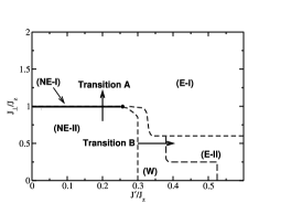
(a) Phase diagram of (3) in the $J^{\prime}-J_{\perp}$ plane.

(b) Transition A: $J^{\prime}$ is set to $0.2J_{z}$

(c) Transition B: $J_{\perp}$ is set to $0.5J_{z}$

Figure 1: (a) Schematic phase diagram of the model (3). See Ref. [4] for details. Notice the locations and directions of the lines crossing the two phase transitions. Entanglement measure $\tau_{2}$ across transition A (a) and transition B (b) for different system sizes $L=12,16,20,24$.

2 Model and Method

We measure $\tau_{2}$ in the one-dimensional anisotropic extended Heisenberg model with next-nearest-neighbor interaction on a chain with $L$ sites, subject to periodic boundary conditions:

$$H = -J_{z}\sum_{i}S^{z}_{i}S^{z}_{i+1}+J_{\bot}\sum_{i}(S^{x}_{i}S^{x}_{i+1}+S^{y}_{i}S^{y}_{i+1})$$ (3)

$$+ J^{\prime}\sum_{i}\mathbf{S}_{i}\mathbf{S}_{i+2}.$$

We diagonalize the Hamiltonian (3) by means of the Lanczos diagonalization technique. In doing that we take into account translational symmetry and classify the eigenstates by the eigenvalues of total $S^{z}$ which is a good quantum number. We use $J_{z}>0$, which corresponds to ferromagnetic coupling.

3 Results

The phase diagram in the $J^{\prime}-J_{\perp}$ plane, as found in Ref. [4] and shown on Fig. 1(a), manifests the presence of a totally polarized phase (NE-II phase), which neighbors two paramagnetic phases at the lines $J_{\perp}=J_{z}$ and $J^{\prime}\approx 0.33J_{z}$. In this article we study these two phase transitions, which we will call transition A and transition B, respectively. In the NE-II the ground state is doubly degenerate with all spins either ”up” or ”down” and therefore $\tau_{2}=0$ because this is a product state. The behavior of $\tau_{2}$ across the transition lines for two representative values of $J^{\prime}$ and $J_{\perp}$, is shown in Fig. 1(b)-(c), respectively. We summarize the properties of the two transitions as follows:

Transition A: In this transition frustration, induced by the antiferromagnetic interaction, parametrized by $J_{\perp}$, destroys the ferromagnetic order. If $J_{\perp}>J_{z}$ the system becomes antiferromagnetic in $XY$ plane, as emerges from our analysis [5]. It is clear that such a ground state is entangled. $C_{i,i+d}$ monotonically decreases as a function of $d$, and the main contribution to $\tau_{2}$ comes from the nearest-neighbor term ($d=1$). For the system sizes considered, $L=12\div 24$, the decay of the antiferromagnetic correlations is very weak and they scale well with increasing $L$. This fact explains the good finite-size scaling of our results for $\tau_{2}$.

Transition B: In the definition of the concurrence (1) it might happen that for some $d$ there is no dominant eigenvalue of $R$ and $C_{i,i+d}=0$. This would mean that for this particular $d$ the two spins are untangled from the rest of the system. This is the case of the phase, situated behind the transition B. Precisely, the only non-zero contribution to $\tau_{2}$ comes from $d=2$. This implies the enhancement of correlations at $d=2$, as indeed found by examining the correlation functions. This feature is short-ranged even for the small sizes considered here and persists both in $Z-$direction and in $XY$ plane. Within the range of $J^{\prime}$ considered [$0.3J_{z},0.4J_{z}$] there are regions, characterized by a finite magnetisation per site less than $1/2$. For $J^{\prime}\gtrsim 0.37J_{z}$ the magnetisation stabilizes at zero. It is this finite magnetisation which is responsible for the steps of $\tau_{2}$ on the right panel of Fig. 1(c). Unfortunately our computation facilities did not allow us to conclude whether these steps are a finite-size effect, and whether the vanishing of the ground state magnetisation at the QPT is continuous or not. The shorter range of the correlations respect to the Transition A case and the presence of the magnetisation steps imply a worse finite-size scaling in this case.

In conclusion, we have studied the entanglement change across two QPTs in the vicinity of the ferromagnetic phase in the extended anisotropic Heisenberg model (3). The entanglement appears to be intimately connected to the underlying ground state of the system. Starting from a totally untangled ferromagnetic state, by changing the Hamiltonian parameters, we observed the complete reordering of the ground state structure. Such reordering is accompanied by the appearance of pairwise entanglement, reflecting the structure of underlying ground state. Namely, in the transition A, entanglement is non-zero for all the distances, being maximal for nearest neighbors, while for transition B only the next-nearest-neighbor entanglement is non-zero.

References

- [1] For review see e.g. L. Amico et al. quant-ph/0703044v1 (2007).
- [2] Wootters, W. K., Phys. Rev. Lett. 80, 2245 (1998).
- [3] V. Coffman et al., Phys. Rev. A 61, 052306 (2000).
- [4] E. Plekhanov, A. Avella, and F. Mancini Phys. Rev. B 74, 115120 (2006).
- [5] E. Plekhanov, A. Avella, and F. Mancini: the detailed analysis of the ground state phase diagram, in view of the brevity of the present article will be published elsewhere.