Neutral Hydrogen Absorption Toward XTE J1810–197: the Distance to a Radio-Emitting Magnetar

Abstract

We have used the Green Bank Telescope to measure H I absorption against the anomalous X-ray pulsar XTE J1810–197. Assuming a flat rotation curve, we find that XTE J1810–197 is located at a distance of $3.4_{-0.7}^{+0.5}$ kpc. For a rotation curve that incorporates a model of the Galactic bar, we obtain a distance of $4.0_{-0.8}^{+0.3}$ kpc. Using a rotation curve that incorporates a model of the Galactic bar and the spiral arms of the Galaxy, the distance is $3.7\pm 0.6$ kpc. These values are consistent with the distance to XTE J1810–197 of about 3.3 kpc derived from its dispersion measure, and estimates of 2–5 kpc obtained from fits to its X-ray spectra. Overall, we determine that XTE J1810–197 is located at a distance of $3.5\pm 0.5$ kpc, possibly not far in front of the infrared dark cloud G10.74–0.13 (catalog ). We also used the GBT in an attempt to measure absorption in the OH ${\rm{}^{2}\pi_{3/2}(J=3/2)}$ lines against XTE J1810–197. We were unsuccessful in this, mainly because of its declining radio flux density. Analysis of H I 21 cm, OH ${\rm{}^{2}\pi_{3/2}(J=3/2)}$, and ¹²CO$(2\rightarrow 1)$ emission toward XTE J1810–197 allows us to place a lower limit of $N_{\rm H}\gtrsim 4.6\times 10^{21}$ cm^-2 on the non-ionized hydrogen column density to XTE J1810–197, consistent with estimates obtained from fits to its X-ray spectra.

1 Introduction

Prior to the detection of pulsed radio emission from the anomalous X-ray pulsar (AXP) XTE J1810–197 by Camilo et al. (2006), pulsed emission from the dozen known magnetars had been detected in X-rays in all instances, and in one case at optical wavelengths. Estimating the distance to a magnetar has relied on associating it with a supernova remnant (SNR) of known distance, or by fitting its X-ray spectrum and parameterizing the energy-dependent absorption by interstellar gas along the line of sight with a non-ionized hydrogen column density $N_{\rm H}$ (Morrison & McCammon, 1983). Using standard relations, $N_{\rm H}$ is related to visual extinction $A_{V}$, which is turned into a distance estimate using mean values in the Galactic plane (see, e.g., §6 of Gotthelf et al., 2004), or is directly calibrated as a function of distance using stars of known luminosity in the field (Durant & van Kerkwijk, 2006). Sometimes, the probable location of the X-ray source in a well-studied star cluster can be used to infer its distance (Muno et al., 2006).

The unique detection of pulsed radio emission from XTE J1810–197 allows one to determine its distance using methods that are not applicable to other magnetars. The dispersion measure (DM, the total column density of free electrons along the line of sight) was obtained upon discovery of the radio pulsations (Camilo et al., 2006). A model for the Galactic free electron distribution then yields a distance estimate, in this case $d\approx 3.3$ kpc using the most recent model (Cordes & Lazio, 2002). Also, bright, pulsed radio emission allows kinematic distance limits to be obtained by observing spectral lines that are seen in absorption against the magnetar, as we report here using H I.

Obtaining a reliable distance to XTE J1810–197 allows for a precise determination of the luminosity of the star based on its measured flux in a variety of wavebands. The distance also allows a proper motion (see Helfand et al., 2007) to be converted into a tangential velocity. Magnetars are thought to be very young neutron stars, and are expected to be found near star forming regions and/or spiral arms. Knowing the distance to XTE J1810–197 allows this prediction to be tested in this case. Besides providing a kinematic distance, the H I absorption spectrum can also give an independent estimate of $N_{\rm H}$, which may be compared to results from X-ray spectral fitting.

In § 2 we present the H I and OH observations and data analysis. This is followed by a determination of the hydrogen absorption spectra toward XTE J1810–197, in § 3, and of its kinematic distance in § 4. In § 5 we comment briefly on some features of the neutral hydrogen toward XTE J1810–197, and in § 6 on the OH absorption limits. We obtain a limit on the hydrogen column density in § 7, and comment on models of the line of sight toward XTE J1810–197 in § 8. We conclude in § 9 with a discussion of our main results.

2 Observations and Data Analysis

2.1 H I 21 cm Absorption Observations

XTE J1810–197 was observed with the National Radio Astronomy Observatory (NRAO) Robert C. Byrd Green Bank Telescope (GBT) for approximately 3 hr on 2006 June 6 in order to measure the H I 21 cm line absorption. The GBT has an unblocked aperture, a spatial resolution of $9\farcm 2$ at 21 cm, and a system temperature on cold sky of 18 K. The NRAO spectral processor (SP), an FFT spectrometer, was used as the detector. The SP provides good dynamic range for the observations via its 32-bit sampling, and was used in its pulsar mode whereby it accumulates spectra that are folded synchronously with the pulsar period. The SP was configured to have 1024 channels for each linear polarization across a bandwidth of 2.5 MHz, producing a spectral resolution of 0.52 km s^-1 per channel. We recorded 128 spectra (phase bins) evenly spaced in time across each individual period of XTE J1810–197. The duty cycle of this 5.54 s pulsar was such that 4–5 of these bins contained pulsed flux.

2.2 OH ${\rm\bf{}^{2}\pi_{3/2}(J=3/2)}$ Absorption Observations

XTE J1810–197 was observed with the GBT for approximately 38 hr in order to measure absorption in the 1612, 1665, 1667 and 1720 MHz ${\rm{}^{2}\pi_{3/2}(J=3/2)}$ ground state transitions of OH. Observing details are given in Table 1. The GBT’s angular resolution is approximately $8^{\prime}$ for each of the OH transitions. The spectral processor was also used for these measurements and was configured to provide 256 spectral channels for each linear polarization across each of the four OH transitions. A bandwidth of 0.625 MHz was used, giving a spectral resolution of 0.44 km s^-1 per channel. We chose this narrower bandwidth (with higher frequency resolution) since we already knew which velocities displayed H I absorption. As with the H I measurements, the pulsed flux of XTE J1810–197 was detected in 4–5 phase bins.

The GBT auto-correlation spectrometer (ACS) was used to obtain pulsar “off” spectra for the four OH lines. The data were obtained in six position-switching observations, each consisting of two minutes on source followed by two minutes off source, resulting in an effective integration time of 12 minutes. An off position two minutes of time in R.A. offset from the position of XTE J1810–197 was used so that approximately the same hour-angle coverage was obtained for the on and off positions. The ACS was configured to observe all four of the OH ${\rm{}^{2}\pi_{3/2}(J=3/2)}$ lines simultaneously with 8192 channels within a bandwidth of 12.5 MHz, resulting in a spectral resolution of 0.27 km s^-1. These observations allow for a better calibration of the pulsar “off” OH spectra.

2.3 Data Reduction

The data were analyzed using a method similar to that described in Weisberg (1978) and Minter et al. (2005). For each individual pulse of XTE J1810–197 and for each spectral line we measured the flux $T(\nu,\phi,\mathcal{P})$ in terms of the equivalent brightness temperature $T$, versus frequency $\nu$, phase $\phi$ across the pulse (equivalent to time), and polarization $\mathcal{P}$. For each polarization and pulse, the data were divided into two separate parts, a pulsar “on” spectrum and a pulsar “off” spectrum:

$${T_{\rm on}(\nu,\mathcal{P})} = {{\sum_{\phi_{\rm on}}\left(T(\nu,\phi_{\rm on},\mathcal{P})\left[{\left<T(\nu,\phi_{\rm on},\mathcal{P})\right>_{\nu({\rm noabs})}\over T_{\rm sys}}\right]^{2}\right)\over\sum_{\phi_{\rm on}}\left[{\left<T(\nu,\phi_{\rm on},\mathcal{P})\right>_{\nu(\rm noabs)}\over T_{\rm sys}}\right]^{2}}}$$ (1)

$${T_{\rm off}(\nu,\mathcal{P})} = {{\sum_{\phi_{\rm off}}T(\nu,\phi_{\rm off},\mathcal{P})\over N_{\phi_{\rm off}}}}$$ (2)

where ${\phi_{\rm on}}$ are the phase bins when the pulsar is on, ${\phi_{\rm off}}$ are the phase bins when the pulsar is off, ${N_{\phi_{\rm off}}}$ is the total number of phase bins when the pulsar is off and ${\rm\left<\right>_{\nu({\rm noabs})}}$ denotes averaging over the frequencies that do not show absorption in the final spectrum. A pseudo-absorption spectrum for the $i$th pulse is then formed by taking the difference between the pulsar on and pulsar off spectra,

$$T_{\rm on}^{i}({\nu},\mathcal{P})-T_{\rm off}^{i}({\nu},\mathcal{P})=\left(T_{\rm p}^{i}(\nu,\mathcal{P})e^{-\tau(\nu)}+T_{\rm H~{}I}({\nu})+T_{\rm sys}\right)-\left(T_{\rm H~{}I}({\nu})+T_{\rm sys}\right)$$

$$=T_{\rm p}^{i}(\nu,\mathcal{P})e^{-\tau(\nu)}$$ (3)

where ${T_{\rm p}}$ is the brightness temperature of the pulsar. We then take a weighted average of the pseudo-absorption spectrum

$${\left<T_{\rm p}(\nu,\mathcal{P})\right>e^{-\tau(\nu)}={\sum_{i}\left(T_{\rm p}^{i}(\nu,\mathcal{P})e^{-\tau(\nu)}\left[{\left<T_{\rm p}^{i}(\nu,\mathcal{P})\right>_{\nu}({\rm noabs})\over T_{\rm sys}}\right]^{2}\right)\over\sum_{i}\left[{\left<T_{\rm p}^{i}(\nu,\mathcal{P})\right>_{\nu}({\rm noabs})\over T_{\rm sys}}\right]^{2}}}$$ (4)

and store the weights for later use when the polarizations are averaged together. This weighting is proportional to the signal-to-noise ratio obtained for each pulse of XTE J1810–197. A third-order orthogonal polynomial was fitted to the $\left<T_{\rm p}(\nu,\mathcal{P})\right>e^{-\tau(\nu)}$ spectrum in order to determine the intrinsic pulsar brightness, $T_{\rm p}^{\rm fit}(\nu,\mathcal{P})$, at all frequencies, i.e., by extrapolating $\left<T_{\rm p}(\nu,\mathcal{P})\right>$ across the absorption features. This yielded the absorption spectrum

$$e^{-\tau({\nu})}={\left<T_{\rm p}(\nu,\mathcal{P})\right>e^{-\tau(\nu)}\over T_{\rm p}^{\rm fit}({\nu,\mathcal{P}})}$$ (5)

for each polarization. The absorption spectra for the different polarizations were then averaged using the weights from equation (4) to create the final, measured absorption spectrum for each spectral line.

For the H I data, the pulsar off spectrum (i.e., the normal H I emission spectrum) was converted from detector counts to a Kelvin scale using a calibrated noise diode that was injected during two-minute calibration scans. Observations of the IAU H I standard source S6 were also made to put the pulsar off spectrum on the IAU standard brightness temperature scale.

3 The Absorption Spectra Toward XTE J1810–197

The H I absorption spectrum toward XTE J1810–197 is shown in Figure 1. XTE J1810–197 is highly linearly polarized (Camilo et al., 2007b) so that the YY polarization signal had a much better signal-to-noise ratio (by a factor of $\approx 4$) than the XX polarization. The two polarizations were averaged together with weights given by their signal-to-noise ratios to produce the spectrum shown. The spectrum has not been smoothed in any way and shows the native resolution of the observations.

Five Gaussians were fitted to the opacities determined from the H I absorption toward XTE J1810–197. The results of the fit are shown in Table 2 and in Figure 2. The columns in Table 2 give for each line, respectively, the opacity, Local Standard of Rest velocity ($V_{\rm LSR}$), and full-width at half-maximum (FWHM). The errors listed in Table 2 are $1\,\sigma$ errors from the Gaussian fits.

The $V_{\rm LSR}=7.7$ km s^-1 absorption line is associated with the Heeschen Cloud (Riegel & Crutcher, 1972), which has also been called the Riegel–Crutcher Cloud by McClure-Griffiths et al. (2006). The Heeschen Cloud is a nearby, $d\approx 125\pm 25$ pc, cold cloud ($T_{\rm spin}\approx 40$ K) that covers Galactic longitudes $345^{\circ}$ to $25^{\circ}$ and latitudes $\pm 6^{\circ}$. This cloud is also seen as a self-absorption feature in the H I emission spectrum (top panel of Fig. 1). The weak absorption line at $V_{\rm LSR}=14.1$ km s^-1 can be kinematically associated with gas in the Carina–Sagittarius spiral arm assuming that the line arises on the near side of the tangent point and using the Galactic rotation model of Englmaier & Gerhard (2006). Likewise, the $V_{\rm LSR}=22.8$ and 25.7 km s^-1 lines can be kinematically associated with the Crux–Scutum spiral arm.

The OH absorption spectra toward XTE J1810–197 are shown in Figures 3–6. With the strength of the pulsar emission during the OH measurement epochs being much weaker than was the case for the H I measurement epoch (Camilo et al., 2007a), the strong linear polarization of XTE J1810–197 means that only one polarization effectively contributed to the measurement of the OH absorption against XTE J1810–197. Thus, the OH absorption data shown in Figures 3–6 and discussed in this paper are only from a single linear polarization (YY). The $1\sigma$ opacity limits for any OH absorption toward XTE J1810–197 are given in Table 3.

4 Determining the Kinematic Distance to XTE J1810–197

4.1 Near or Far Side of the Velocity–Distance Relationship?

XTE J1810–197 is located at Galactic coordinates $(l,b)=10\fdg 726,-0\fdg 158$. At this Galactic longitude the kinematic velocity–distance relationship is double-valued (see Fig. 7). Our first concern is whether it is possible to determine on which side of the tangent point XTE J1810–197 lies. At this Galactic longitude, the tangent point is about 8.3 kpc from the Sun and has a $V_{\rm LSR}\approx 168$ km s^-1 using the flat rotation curve of Burton (1988). Distance estimates for XTE J1810–197 based on its X-ray-fitted $N_{\rm H}$ are 2.5–5 kpc (Gotthelf et al., 2004; Gotthelf & Halpern, 2005; Durant & van Kerkwijk, 2006), and the DM-based distance is 3.3 kpc (Camilo et al., 2006). These strongly suggest that XTE J1810–197 lies on the near side of the tangent point.

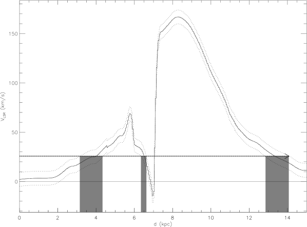
Figure 8: The same as Fig. 7, except that it uses the Galactic rotation model of Weiner & Sellwood (1999), considering potential due to a bar.

Another magnetar, SGR 1806–20 (catalog ), which lies $41^{\prime}$ from XTE J1810–197, has H I absorption at velocities greater than $V_{\rm LSR}=50$ km s^-1 and is thought to lie on the far side of the tangent point (McClure-Griffiths & Gaensler, 2006). Both SGR 1806–20 (catalog ) and the Galactic SNR G11.2–0.3 (catalog ) (Becker et al., 1985) also have H I absorption features at negative velocities that must arise from the far side of the Galactic disk if the rotation curve is flat. However, as the Galactic rotation model of Weiner & Sellwood (1999) shows, these negative velocities can also arise in the Galactic bar at a distance of 7 kpc toward these sources. The Galactic bar induces large radial motions that deviate from the normally assumed circular Galactic rotation. Along the line of sight to XTE J1810–197, the Galactic bar is responsible for motions $>90$ km s^-1 more negative than the prediction of a flat rotation curve (see Fig. 8). Negative-velocity H I absorption is not found toward XTE J1810–197, which according to this model establishes an upper-limit to its distance of 7 kpc (i.e., it is closer than the Galactic bar). This strengthens the conclusion that XTE J1810–197 lies on the near side of the tangent point.

4.2 Is the Last Absorption Feature at the Actual Distance or a Lower Limit?

The number of H I absorption features per kpc in the inner Galaxy is about 1–3 (Garwood & Dickey, 1989, see their Table 3). Assuming a flat rotation curve and a distance of 5 kpc, corresponding to a maximum $V_{\rm LSR}\approx 40$ km s^-1, along with a line width of 3 km s^-1 for the average H I absorption feature, we expect that 38%–100% of the velocities within $V_{\rm LSR}=0$–40 km s^-1 should contain H I absorption along the line of sight toward XTE J1810–197. If $\sim 38$% of the velocity space were occupied by absorption features, then the highest velocity feature in the absorption spectrum toward XTE J1810–197 should be taken as indicating a lower limit for the distance, since there is likely a significant distance between XTE J1810–197 and the H I-absorbing cloud nearest it. If on the other hand the whole velocity range should contain H I absorption, it is likely that the last absorbing feature gives the actual distance to XTE J1810–197.

It is useful to look at absorption measurements toward objects near XTE J1810–197 in order to help us determine the H I absorption velocity coverage. The line of sight to XTE J1810–197 lies near that to the giant Galactic H II complex W 31 (catalog ) (see Fig. 1 of Corbel & Eikenberry, 2004). W 31 (catalog ) is comprised of several individual H II regions including G10.2–0.3 (catalog ), G10.3–0.1 (catalog ), and G10.6–0.4 (catalog ). Roughly on the opposite side of W 31 (catalog ) from XTE J1810–197 lies G10.0–0.3 (catalog ), the wind-blown bubble of LBV 1806–20 (catalog ), and SGR 1806–20 (catalog ). At higher Galactic longitude than XTE J1810–197 lies the SNR G11.2–0.3 (catalog ). All of these objects have H I absorption measurements, except for G10.0–0.3 (catalog ) and LBV 1806–20 (catalog ), which have ${\rm NH_{3}}$ absorption measurements (Corbel & Eikenberry, 2004).

Becker et al. (1985) claimed that SNR G11.2–0.3 (catalog ) lies well on the far side of the tangent point. However, Green et al. (1988) noted the lack of absorption between $V_{\rm LSR}=45$ km s^-1 and the tangent point velocity, which led them to assign a distance of $\approx 5$ kpc to G11.2–0.3 (catalog ), while attributing weak absorption at negative velocities to peculiar motions in local gas. A distance of $\approx 5$ kpc is also in reasonable agreement with the expected expansion of the SNR (Green et al., 1988). If we take the Galactic bar into account using the model of Weiner & Sellwood (1999), we can reconcile the H I absorption with the expansion/age-derived distance estimate of Green et al. (1988). The H I absorption to G11.2–0.3 (catalog ) at $V_{\rm LSR}\approx-20$ km s^-1 arises from the Galactic bar, which is at a distance of $\approx 5.5$–7.0 kpc along this line of sight (see Fig. 8). With both the Galactic bar and G11.2–0.3 (catalog ) being on the near side of the tangent point toward G11.2–0.3 (catalog ), H I absorption is not expected at $V_{\rm LSR}>45$ km s^-1. So we judge that G11.2–0.3 (catalog ) likely lies within the Galactic bar at $\approx 5.5$–7 kpc.

Corbel & Eikenberry (2004) determined that G10.3–0.1 (catalog ), G10.0–0.3 (catalog ), LBV 1806–20 (catalog ), and SGR 1806–20 (catalog ) all lie on the far side of the tangent point, while G10.2–0.3 (catalog ) and G10.6–0.4 (catalog ) lie on the near side. The H I absorption of G10.3–0.1 (catalog ) (Fig. 2 of Kalberla et al., 1982) and SGR 1806–20 (catalog ) (Fig. 2 of Cameron et al., 2005) fill the range $V_{\rm LSR}=0$–40 km s^-1. H I toward G10.6–0.4 (catalog ) shows absorption at all velocities within $V_{\rm LSR}=0$–45 km s^-1 (Fig. 32 of Caswell et al., 1975). Likewise, the H I absorption toward G10.2–0.3 (catalog ) (Fig. 4 of Greisen & Lockman, 1979) and SNR G11.2–0.3 (catalog ) (Fig. 3 of Becker et al., 1985) completely cover the velocity range $V_{\rm LSR}=0$–45 km s^-1. Since G10.6–0.4 (catalog ), G10.2–0.3 (catalog ) and G11.2–0.3 (catalog ) all lie on the near side of the tangent point and are only $16\arcmin$, $33\arcmin$ and $30\arcmin$, respectively, in projection from XTE J1810–197, we argue that all velocities between the Sun and XTE J1810–197 should show H I absorption. Therefore, the highest-velocity absorption feature seen along the line of sight toward XTE J1810–197 gives us its true distance, rather than a lower limit.

4.3 The Kinematic Distance to XTE J1810–197

For the kinematic distance models that we discuss we will assume that the Sun is located 8.5 kpc from the Galactic center. We will also use a velocity of $V_{\sun}=220$ km s^-1 as the azimuthal velocity of the LSR about the Galactic center. These are the current IAU standards. However, there is evidence that these values may not be correct (see the discussions in Reid, 1993; Englmaier & Gerhard, 2006), which would require a scaling of the kinematic distance estimates presented below.

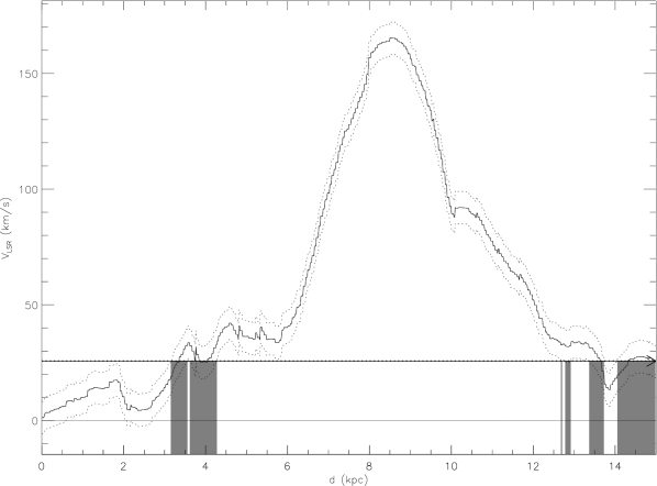
Figure 9: The same as Fig. 7, except that it uses the Galactic rotation model of Englmaier & Gerhard (2006), considering potential due to a bar and spiral arms.

In Figure 7 we show the determination of the distance to XTE J1810–197 using the flat rotation curve of Burton (1988). Cold H I clouds have random motions superposed on the uniform Galactic rotation as indicated by their measured velocity dispersion of 7 km s^-1 (Lockman & Dickey, 1990). The dotted lines on either side of the rotation model in Figure 7 indicate the deviation from Galactic rotation of $\pm 7$ km s^-1. (The random motions of the clouds are relative to the Galactic rotation and not to the measured velocity of the cloud. Thus, the 7 km s^-1 represents an error in converting the model’s distance into a velocity and not in using the measured velocity of the cloud to obtain a distance as is usually presumed. This distinction can be quite important in determining the distance and its errors when the observed velocity is at or near a local maximum or minimum in the model. However, in most cases it makes only a minor difference.) The arrow at a constant $V_{\rm LSR}$ in Figure 7 indicates the velocity of the highest velocity H I absorption. The shaded regions in Figure 7 indicate the allowed kinematic distances from the flat rotation curve. Figures 8 and 9 are similar to Figure 7, using instead the Galactic rotation models of Weiner & Sellwood (1999) and Englmaier & Gerhard (2006), respectively.

For the flat rotation curve used in Figure 7, the last H I absorption feature toward XTE J1810–197 at $V_{\rm LSR}=25.7$ km s^-1 (see Table 2) gives a kinematic distance of $3.4_{-0.7}^{+0.5}$ kpc or $13.3_{-0.5}^{+0.7}$ kpc. We can rule out the larger distance since this is on the far side of the tangent point. Although a flat rotation model may provide a reasonable distance estimate for XTE J1810–197, there are Galactic structures along the line of sight that also need to be taken into account. Spiral arms can have a substantial effect on the expected Galactic rotational velocities (Roberts, 1972). The Galactic bar may also have an influence by adding non-circular motions to the general Galactic rotation.

The rotation model of Weiner & Sellwood (1999) used in Figure 8 takes into account the effects of a strong potential associated with the Galactic bar. This model uses a global Galactic gravitational potential to determine the motions of the gas in the ISM. It uses both the minimum and maximum observed H I velocities along lines of sight in the inner Galaxy in fitting the properties of the Galactic potential. We can again immediately rule out the distance on the far side of the tangent point. Since no H I absorption is seen at velocities between 30 and 40 km s^-1 (see Table 2) we can eliminate all distances except $4.0_{-0.8}^{+0.3}$ kpc. The Weiner & Sellwood (1999) model, however, does not take into account the effects of spiral arms. Since magnetars are expected to lie in or near spiral arms this could have a significant impact on the velocity-determined distance to XTE J1810–197.

The rotation model of Englmaier & Gerhard (2006) used in Figure 9 takes into account the effects of a potential associated with the Galactic bar as well as those associated with spiral arms. The Englmaier & Gerhard (2006) model was determined in a similar fashion as the Weiner & Sellwood (1999) model. However, in the Englmaier & Gerhard (2006) model only the maximum (minimum) observed velocities for CO were used for positive (negative) Galactic longitudes. It should be noted that CO observations do not trace column densities as low as H I does. Combined with fitting to only one side of the velocity–longitude data, this means that the Englmaier & Gerhard (2006) model uses a weaker potential for the Galactic bar compared with the Weiner & Sellwood (1999) model. In fact, the Englmaier & Gerhard (2006) model predicts that there should be no negative velocity gas along the line of sight toward XTE J1810–197, while the Weiner & Sellwood (1999) model does. As can be seen in the Southern Galactic Plane Survey H I data (McClure-Griffiths et al., 2005), there is plenty of gas at negative velocities along this line of sight. We suggest that the Englmaier & Gerhard (2006) Galactic bar potential is too weak and that the Weiner & Sellwood (1999) model should be used for velocities and distances associated with the Galactic bar.

We can, however, still use the Englmaier & Gerhard (2006) model to determine a distance for XTE J1810–197 since it is likely located in front of the Galactic bar as is evidenced by the Weiner & Sellwood (1999) model results from above. In fact, comparing the Englmaier & Gerhard (2006) result with the Weiner & Sellwood (1999) result provides an indication of how spiral arms may be affecting the velocity–distance relationship toward XTE J1810–197. We can again rule out distances that lie on the far side of the tangent point and distances that include 30–40 km s^-1 gas along the line of sight. As can be seen from Figure 9, we obtain kinematic distances of $3.3_{-0.2}^{+0.2}$ kpc or $4.0_{-0.4}^{+0.3}$ kpc. Due to uncertainties in the modeling of the Galactic rotation curve, the $0.1$ kpc gap in distance between these two values is in effect negligible. We thus combine these two possible distance ranges into a single value, $3.7\pm 0.6$ kpc.

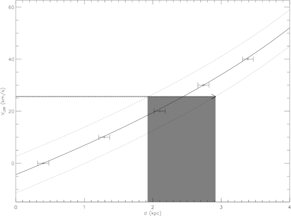
Figure 10: The same as Fig. 7, except that it uses the Galactic rotation model of Brand & Blitz (1993), derived from observations of H II regions. The points and error bars are derived from Fig. 2 of Brand & Blitz (1993). The solid line is a quadratic fit to the points.

All of the above Galactic rotation models are derived from empirical models fit to observed data. There is one model that is fully derived from observational data, that of Brand & Blitz (1993). In this model, observations of H II regions are used. The velocities of the H II regions are determined from recombination lines and H I absorption. Independent measurements provide distances to the H II regions. Using the rotation model of Brand & Blitz (1993), shown in Figure 10, we obtain $d=2.4\pm 0.5$ kpc. However, this model does not have enough H II regions at $d\gtrsim 2$ kpc in the general direction of XTE J1810–197 to be able to provide a good velocity–distance relation (see Brand & Blitz, 1993), so we give it little weight.

We conclude that the best estimate of a kinematically determined distance to XTE J1810–197 is provided by the Weiner & Sellwood (1999) and Englmaier & Gerhard (2006) models, giving $d=$ 3.1–4.3 kpc.

5 The Neutral Hydrogen Toward XTE J1810–197: GBT Versus SGPS

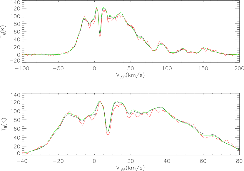
Figure 11: Comparison of the GBT H I spectrum (black line) with the full-resolution SGPS H I spectrum (red line) toward XTE J1810–197. The SGPS spectrum convolved to the same resolution as the GBT is shown as the green line. The top panel shows the full range of emission, while the lower panel is zoomed in to show the difference in line widths for the Heeschen Cloud absorption around 8 km s^-1.

The GBT has a resolution of $9\farcm 2$ at 21 cm while the Southern Galactic Plane Survey (SGPS, McClure-Griffiths et al., 2005) has a resolution of about $3\farcm 3$. In Figure 11 we compare the GBT H I spectrum with the SGPS spectrum. For the H I self-absorption associated with the Heeschen Cloud we find the remarkable result that the line width of the absorption increases with increasing spatial resolution! To our knowledge this effect has never been observed before for H I on arc-minute resolutions.

Inspection of the SGPS H I data cube shows that there is structure within the H I emission inside of the GBT beam. We convolved the SGPS data with a beam the size of GBT’s, so that the two data sets would have the same spatial resolution. As can be seen from Figure 11 the GBT spectrum and $9\farcm 2$ resolution SGPS spectrum are in very good agreement. If we compare the line width of the H I absorption due to the Heeschen Cloud at $\sim 8$ km s^-1 with the SGPS data having H I absorption seen against XTE J1810–197, we find that the line widths are identical.

These properties suggest that there is definite spatial structure in the H I emission on size scales of $3\farcm 3$ to $9\farcm 2$ (0.12–0.33 pc for a Heeschan Cloud distance of $d=125$ pc). That the tiny beam of absorption against the magnetar (limited by the size of the pulsar emission region, which is smaller than the pulsar’s light-cylinder radius, or about 1 light-second) has the same line width as the $0.12$ pc-wide beam of the SGPS at the Heeschen Cloud, suggests that there are few if any spatial structures left unresolved by the SGPS in the Heeschen Cloud. Since the H I self-absorption line width does change between the GBT and SGPS resolutions we can infer that either the absorption feature comprises multiple narrow line features or that the non-thermal broadening of the absorption feature changes between different structures in the Heeschen cloud. Attempts to fit the different line-width absorption-line structures in the Heeschen cloud with multiple Gaussian components does not improve the fitting, which suggests that a single Gaussian is sufficient. This implies that the non-thermal contribution to the line width varies within the cloud.

The standard assumption is that non-thermal line broadening arises from turbulence. If the turbulence is intermittent, we can expect that the turbulence has decayed more in some places than in other locations (Frisch, 1995). This can then easily explain the observed line widths of the Heeschen Cloud H I absorption. The areas that have undergone more damping of the turbulence will have less turbulent energy and thus have narrower non-thermal line widths.

6 OH Absorption Limits Toward XTE J1810–197

Although we did not detect any OH absorption against XTE J1810–197, the limits are still interesting. All previous OH absorption detections against pulsars (Stanimirović et al., 2003; Weisberg et al., 2005; Minter, 2005) have found that the absorption is deeper (larger opacity) and has a narrower line width than the pulsar “off” spectra: in the three known cases, the OH absorption against the pulsar is 2–3 times deeper than seen in the pulsar off spectra.

For our OH absorption limits against XTE J1810–197 of $\tau<0.1$ ($1\,\sigma$), we would expect our pulsar off spectra to have OH opacities $\lesssim 0.033$. In Table 4 we list the opacities of the OH lines in the pulsar off spectra. We subtracted the system temperature from the raw OH spectra, and then fitted a third order polynomial to determine the continuum emission levels. Dividing the spectra by the continuum emission results in $e^{-\tau}$ spectra for the pulsar off spectra.

If we assume that the OH pulsar off spectra should have a factor of 2–3 weaker opacity than the OH absorption against the pulsar, then we were likely within a factor of about 2 of detecting OH absorption against XTE J1810–197 at velocities within the range observed for H I absorption (Table 2), e.g., at 9.9 km s^-1 at 1612 MHz, and 9.8 and 16.9 km s^-1 at 1720 MHz (see Table 4). Unfortunately, due the decay of the flux of XTE J1810–197 (Camilo et al., 2007a), we were not able to detect any OH absorption.

Our OH absorption limits toward XTE J1810–197 are also meaningful for the OH seen at $V_{\rm LSR}\gtrsim 28$ km s^-1. The 1665 MHz OH feature at 30.7 km s^-1 should have been detected at 2–$3\,\sigma$ if it were between us and XTE J1810–197. However, we would not have expected to detect OH absorption at these velocities based on the H I absorption results (Table 2).

7 The Column Density to XTE J1810–197

From the H I and OH observations that we have performed, it is possible to estimate the column density of hydrogen $N_{\rm H}$, both atomic and molecular, to XTE J1810–197. This can then be compared with the range of values $N_{\rm H}=(6.5$–14$)\times 10^{21}$ cm^-2 determined from fitting X-ray spectra (Gotthelf & Halpern, 2005; Durant & van Kerkwijk, 2006).

7.1 Estimate of the Atomic Column Density to XTE J1810–197

We cannot directly measure the H I column density toward XTE J1810–197, since we do not have enough constraints to perform radiative transfer modeling in this direction. We can however still make an estimate of the column density to XTE J1810–197. To do this, we just integrate the H I emission spectrum between 0 and 25.7 km s^-1. Assuming that half of the emission at a given velocity comes from H I on the near side of the tangent point and the other half comes from gas with similar properties on the far side of the tangent point, we obtain an estimate of the column density to XTE J1810–197,

$$N_{\rm HI}={1\over 2}\int_{0}^{25.7}1.83\times 10^{18}~{}T_{\rm B}(v)~{}dv.$$ (6)

Since there are clouds on the near side of the tangent point that significantly absorb the H I emission from the far side of the tangent point, as is evidenced by the absorption seen against XTE J1810–197, this method provides a lower limit to the column density of H I to XTE J1810–197. Upon performing the integration we find that $N_{\rm HI}\gtrsim 1.8\times 10^{21}$ cm^-2.

7.2 Estimate of the Molecular Column Density to XTE J1810–197

We can use the pulsar “off” OH spectra to make an estimate of the molecular column density to XTE J1810–197. From Figures 3 and 6 we see that the 1612 MHz OH lines are in absorption while the 1720 MHz OH lines are in emission, with both having approximately the same amplitude. Such conjugate emission arises in regions where the OH column density is in the range $10^{14}<N_{\rm OH}/\Delta v<10^{15}$ cm^-2 km^-1 s with $\Delta v$ the velocity resolution of the observations (Weisberg et al., 2005; Elitzur, 1992). The total column density of OH is found by integrating over the whole line.

Integrating over the OH spectrum between 0 and 25.7 km s^-1 and assuming that half of the OH emission is from beyond the tangent point, we find

$$(2.4\pm 0.3)\times 10^{14}<N_{\rm OH}<(2.4\pm 0.3)\times 10^{15}~{}{\rm cm}^{-2}.$$

Using standard abundances, the ratio of the number of OH molecules to the number of hydrogen atoms is $N_{\rm OH}/N_{\rm H}=6\times 10^{-8}$ (Elitzur, 1992), which gives

$$(4\pm 0.7)\times 10^{21}<N_{\rm H}<(40\pm 7)\times 10^{21}~{}{\rm cm}^{-2}$$

between us and the magnetar.

Measurements of the ¹²CO$(2\rightarrow 1)$ spectrum toward XTE J1810–197 are available from Dame et al. (2001). The total column density of hydrogen in molecular form can be determined from the ¹²CO$(2\rightarrow 1)$ spectrum using

$${N_{\rm H}=2N_{\rm H_{2}}=X_{\rm CO}\int_{0}^{25.7}T_{\rm B}^{\rm CO}(v)dv}$$ (7)

where $X_{{\rm CO}}$ is a conversion factor. The commonly used “standard” value for this is $X_{\rm CO}=2\times 10^{20}$ cm^-2 K^-1 km^-1 s. However, $X_{\rm CO}$ is known to vary depending on the line of sight (Magnani et al., 1998). The ¹²CO$(2\rightarrow 1)$ spectrum nearest to the line of sight toward XTE J1810–197 gives $\int_{0}^{25.7}T_{\rm B}^{\rm CO}(v)dv=28.75$ K km s^-1, of which we will assume that half arises from beyond the tangent point. From Figure 4 of Magnani et al. (1998) we see that $X_{\rm CO}=10^{20}$ cm^-2 K^-1 km^-1 s is reasonable for the amount of ¹²CO$(2\rightarrow 1)$ toward XTE J1810–197. This then yields $N_{\rm H}\gtrsim 2.8\times 10^{21}$ cm^-2.

This limit for $N_{\rm H}$ obtained from the CO spectrum is consistent with the range of values determined using the OH spectra (eq. 7.2). This also tells us that the OH column densities are near the lower limit of $N_{\rm OH}/\Delta v=10^{14}$ cm^-2 km^-1 s. Since the CO spectra have a higher signal-to-noise ratio, we will use the CO value for the molecular gas contribution to $N_{\rm H}$.

Adding the molecular and atomic components of $N_{\rm H}$, we obtain $N_{\rm H}\gtrsim 4.6\times 10^{21}$ cm^-2. This limit is in agreement with the values determined from the X-ray spectrum of XTE J1810–197. Unfortunately we only have a lower limit for the total column density that is below the values determined from the X-ray spectrum.

8 Models of the Line of Sight Toward XTE J1810–197

A detailed molecular model of the ISM toward SGR 1806–20 (catalog ) has been developed by Corbel et al. (1997) and Corbel & Eikenberry (2004), depicted in Figure 8 of the latter. With increasing distance toward SGR 1806–20 (catalog ), their model encounters gas at $V_{\rm LSR}=4$, 24, 30, 38, 44, and then 13 km s^-1 in reaching the Scutum-Crux spiral arm (labeled as the 30 km s^-1 spiral arm in Fig. 8 of Corbel & Eikenberry, 2004). Since the line of sight toward SGR 1806–20 (catalog ) is very close to that of XTE J1810–197 we might expect to encounter clouds at roughly the same velocities on the line of sight toward XTE J1810–197.

The gas at 4 km s^-1 toward SGR 1806–20 (catalog ) is likely one of the two velocity components of the Heeschen Cloud (Riegel & Crutcher, 1972) and can be associated with the H I absorption feature at 7.7 km s^-1 toward XTE J1810–197, which is from the other velocity component of the Heeschen Cloud. The gas at 24 km s^-1 toward SGR 1806–20 (catalog ) can be associated with the H I absorption features at 22.8 or 25.7 km s^-1 toward XTE J1810–197. We can associate the 13 km s^-1 gas toward SGR 1806–20 (catalog ) with the H I absorption seen at 14.1 km s^-1 toward XTE J1810–197.

If the model of Corbel et al. (1997) and Corbel & Eikenberry (2004) is correct, then we should also expect see H I absorption at velocities of roughly 30, 38, and 44 km s^-1 toward XTE J1810–197, since we observe absorption that can be associated with the 13 km s^-1 cloud in their model. In fact, we do not observe any H I absorption against XTE J1810–197 at these velocities. This suggests that either (1) the model of Corbel et al. (1997) and Corbel & Eikenberry (2004) is not entirely correct, or (2) it cannot be applied to the line of sight toward XTE J1810–197, which is only $41^{\prime}$ away, or (3) there is molecular material without H I along these lines of sight. The last possibility is not likely since molecular clouds are expected to have cosmic-ray ionization and photo-dissociation regions within and at their outer edges, which would produce atomic hydrogen (see Minter et al., 2001, § 9.2, and references therein).

9 Discussion

Using the $\mbox{DM}=178\pm 5$ cm^-3 pc measured for XTE J1810–197 (Camilo et al., 2006), its distance according to the Cordes & Lazio (2002) electron density model is 3.3 kpc. This model has a claimed average uncertainty of about 20% which, however, can be much larger for individual objects. For the sake of discussion, we assume an uncertainty of 1 kpc. The electron density model was derived using distances to pulsars that in many cases were determined via H I absorption spectra assuming a flat rotation curve, so that it seems most appropriate to compare the DM–derived distance of $3.3\pm 1$ kpc with our flat rotation curve’s kinematic distance of $3.4_{-0.7}^{+0.5}$ kpc. These two values agree remarkably well and imply that along the line of sight to XTE J1810–197, the Cordes & Lazio (2002) model gives a good representation of the average free electron density out to about 4 kpc.

The distance to XTE J1810–197 has been estimated from X-ray observations to range over 2.5–5 kpc (Gotthelf & Halpern, 2005; Gotthelf et al., 2004). These distances are determined by converting $N_{\rm H}$ values obtained from fits to the X-ray spectra into visual extinction, $A_{V}$, and an estimate of the $A_{V}$ per kpc in the Galaxy. This method is limited by a number of complications: (1) the spectral model used to fit the X-ray data, e.g., two blackbodies versus a blackbody and a power law; (2) the $N_{\rm H}$ versus $A_{V}$ relationship determined locally (within $\sim 1$ kpc) but used for large distances ($>1$ kpc); (3) the large deviations from the fitted $N_{\rm H}$ versus $A_{V}$ relationship for any particular line of sight; and (4) the $d$–$A_{V}$ relationship also determined locally but used for large distances.

Durant & van Kerkwijk (2006) determined $d=3.1\pm 0.5$ kpc toward XTE J1810–197 assuming an X-ray $N_{\rm H}=14\times 10^{21}$ cm^-2, which is higher than any of the values fitted by Gotthelf et al. (2004) or Gotthelf & Halpern (2005). We consider the $d$–$A_{V}$ relation of Durant & van Kerkwijk (2006) using red clump stars in the line of sight to XTE J1810–197 to be an improvement, although it is still necessary to apply an X-ray–fitted value of $N_{\rm H}$ to this relation and then convert it into a visual extinction $A_{V}$. Using $N_{\rm H}=6.5\times 10^{21}$ cm^-2 determined by Gotthelf & Halpern (2005), which is arguably a lower limit, the extinction toward XTE J1810–197 becomes $A_{V}\approx$ 3–4.5 mag using Figure 3 of Predehl & Schmitt (1995). This then yields a distance estimate of 2–3.5 kpc based on Figure 7 of Durant & van Kerkwijk (2006).

The kinematic distances determined from the H I absorption measurements presented in this paper rely only on the model of Galactic rotation used to convert the measured velocity into a distance. The Weiner & Sellwood (1999) and Englmaier & Gerhard (2006) models both give consistent results (see Table Neutral Hydrogen Absorption Toward XTE J1810–197: the Distance to a Radio-Emitting Magnetar). We prefer the kinematic distance of 3.1–4.3 kpc determined in this paper over the DM- and X-ray-derived distances, because our conversion of measured velocity to distance is more direct and better constrained than through these other methods.

In Figure 7 of Durant & van Kerkwijk (2006) we see that the extinction vs. distance rises steeply between 3.0 and 3.5 kpc and that for $A_{V}\leq 13$ the distance can be limited to be less than 4 kpc. The line of sight toward XTE J1810–197 contains the Infrared Dark Cloud (IRDC) G10.74–0.13 (catalog ) (Simon et al., 2006; Carey et al., 2000). IRDCs are thought to be places where Giant Molecular Clouds are either just starting to form massive stars or on the verge of beginning to form stars. The sudden increase in opacity vs. distance seen by Durant & van Kerkwijk (2006) is likely associated with this IRDC. We note that the highest opacity regions of the IRDC cover less than half the area on the sky that Durant & van Kerkwijk (2006) used to determine the visual extinction vs. distance toward XTE J1810–197. Also, IRDCs can have extremely high opacities such that only the edge of the cloud is seen even in the infrared (Simon et al., 2006; Minter et al., 2001). Since the opacities can be very large, it is plausible that Durant & van Kerkwijk (2006) may have underestimated the actual extinction vs. distance toward XTE J1810–197.

Jaffe et al. (1982) associated IRDC G10.74–0.13 (catalog ) with ${}^{12}{\rm CO}\left(1\rightarrow 2\right)$ emission centered at 32 km s^-1, implying $d<3.8_{-0.5}^{+0.5}$ kpc for a flat rotation curve and $d<4.4_{-0.3}^{+0.6}$ kpc for the Weiner & Sellwood (1999) and Englmaier & Gerhard (2006) models. Our OH spectra show a large spectral feature at the same velocities that we also associate with the IRDC. All observed H I absorption features lie at velocities lower than those associated with the IRDC. This puts XTE J1810–197 no further than the front edge of the IRDC.

We consider the 4 kpc upper limit from Figure 7 of Durant & van Kerkwijk (2006) to be a hard upper limit on the distance to XTE J1810–197. This further constrains slightly the distance estimate of 3.1–4.3 kpc obtained from H I absorption measurements (§ 4.3). Overall, we can thus summarize that the distance to XTE J1810–197 is $3.5\pm 0.5$ kpc. Together with the measured proper motion of the AXP, this results in a transverse velocity corrected to the LSR of $212\pm 35$ km s^-1 (Helfand et al., 2007), a perfectly ordinary velocity among pulsars.

Table 1: Observations of XTE J1810–197 at GBT

Date	Time (UTC)	Species
2006 Jun 6	07:30 – 11:00	H I
2006 Jul 22/23	23:00 – 07:30	OH
2006 Aug 31/Sep 1	23:30 – 05:00	OH
2006 Sep 2	00:00 – 05:00	OH
2006 Sep 4	00:00 – 05:00	OH
2006 Sep 24/25	19:45 – 03:40	OH
2006 Oct 21	17:00 – 19:09	OH
2006 Oct 21/22	20:55 – 01:45	OH

Table 2: Gaussian fits to the H I absorption lines toward XTE J1810–197

$\tau$	$V_{\rm LSR}$	FWHM
	(km s-1)	(km s-1)
$2.15\pm 0.09$	$7.73\pm 0.06$	$3.3\pm 0.2$
$0.5\pm 0.1$	$14.1\pm 0.2$	$1.2\pm 0.4$
$1.53\pm 0.08$	$19.1\pm 0.1$	$3.8\pm 0.4$
$1.2\pm 0.1$	$22.8\pm 0.2$	$2.1\pm 0.4$
$0.94\pm 0.1$	$25.7\pm 0.2$	$2.4\pm 0.5$

Note. — See Figs. 1 and 2 for data upon which these fits are based.

Table 3: OH absorption limits toward XTE J1810–197

$\nu$	$\sigma_{\tau}$
(MHz)
1612	0.09
1665	0.10
1667	0.10
1720	0.10

Table 4: Gaussian fits to the OH opacity in the pulsar “off” spectra toward XTE J1810–197

$\nu$	$\tau$	$V_{\rm LSR}$	FWHM
(MHz)		(km s-1)	(km s-1)
1612	$0.026\pm 0.002$	$9.9\pm 0.2$	$4.4\pm 0.6$
1612	$0.097\pm 0.002$	$29.54\pm 0.05$	$5.4\pm 0.1$
1665	$0.059\pm 0.009$	$28.7\pm 0.5$	$7.9\pm 0.4$
1665	$0.10\pm 0.01$	$30.69\pm 0.08$	$3.9\pm 0.3$
1665	$0.020\pm 0.002$	$39.9\pm 0.3$	$5.5\pm 0.8$
1667	$0.045\pm 0.005$	$28.1\pm 0.6$	$9.7\pm 0.6$
1667	$0.086\pm 0.007$	$31.11\pm 0.08$	$4.3\pm 0.3$
1667	$0.018\pm 0.002$	$42.0\pm 0.4$	$6.3\pm 0.9$
1720	$-0.023\pm 0.002$	$9.8\pm 0.1$	$3.1\pm 0.3$
1720	$-0.020\pm 0.002$	$16.9\pm 0.2$	$4.8\pm 0.5$
1720	$-0.021\pm 0.004$	$26.2\pm 0.2$	$2.3\pm 0.5$
1720	$-0.063\pm 0.002$	$29.5\pm 0.1$	$3.8\pm 0.3$
1720	$0.014\pm 0.002$	$44.4\pm 0.3$	$3.0\pm 0.6$

Table 5: Distance estimates for XTE J1810–197

Measurement	Method	$d$	Refs.
		(kpc)
DM	$n_{e}$ model (Cordes & Lazio, 2002)	$3.3\pm 1$	1
X-ray: blackbody + power law	${N_{\rm H}\rightarrow A_{V}\rightarrow 1.5-2.0~{}{\rm mag\,kpc}^{-1}\rightarrow}d$	$\sim 5.0$	2
X-ray: two blackbodies	${N_{\rm H}\rightarrow A_{V}\rightarrow 1.5-2.0{\rm~{}mag\,kpc}^{-1}\rightarrow}d$	$\sim 2.5$	3
X-ray: blackbody + power law	${N_{\rm H}\rightarrow A_{V}\rightarrow{\rm red~{}clump~{}stars}\rightarrow}d$	$3.1\pm 0.5$	4
X-ray: two blackbodies	${N_{\rm H}\rightarrow A_{V}\rightarrow{\rm red~{}clump~{}stars}\rightarrow}d$	2–3.5	5
H I absorption	Flat rotation curve (Burton, 1988)	$3.4_{-0.7}^{+0.5}$ kpc	5
H I absorption	Weiner & Sellwood (1999) model	$4.0_{-0.8}^{+0.3}$ kpc	5
H I absorption	Englmaier & Gerhard (2006) model	$3.7\pm 0.6$ kpc	5
H I absorption	Brand & Blitz (1993) model	$2.4\pm 0.5$	5

References. — (1) Camilo et al. (2006); (2) Gotthelf et al. (2004); (3) Gotthelf & Halpern (2005); (4) Durant & van Kerkwijk (2006); (5) this work.

Note. — See § 4 for a discussion of the various rotation curve models that we fit to the H I data. The X-ray fits done by other authors are discussed in § 9. Overall, our best distance determination comes largely from the direct H I measurements on XTE J1810–197, and is $3.5\pm 0.5$ kpc (see § 9).

Figure 1: Top: The H I emission spectrum (pulsar “off” spectrum) toward XTE J1810–197. Bottom: The H I absorption spectrum against XTE J1810–197.

Figure 2: Gaussian fits (thick line) to the H I opacity (thin line) observed toward XTE J1810–197. Residuals to the fits are shown as the dotted line. Results of the fits are listed in Table 2.

Figure 3: Top: The OH 1612 MHz pulsar “off” spectrum toward XTE J1810–197. Bottom: The OH 1612 MHz absorption spectrum against XTE J1810–197.

Figure 4: Top: The OH 1665 MHz pulsar “off” spectrum toward XTE J1810–197. Bottom: The OH 1665 MHz absorption spectrum against XTE J1810–197.

Figure 5: Top: The OH 1667 MHz pulsar “off” spectrum toward XTE J1810–197. Bottom: The OH 1667 MHz absorption spectrum against XTE J1810–197.

Figure 6: Top: The OH 1720 MHz pulsar “off” spectrum toward XTE J1810–197. Bottom: The OH 1720 MHz absorption spectrum against XTE J1810–197.

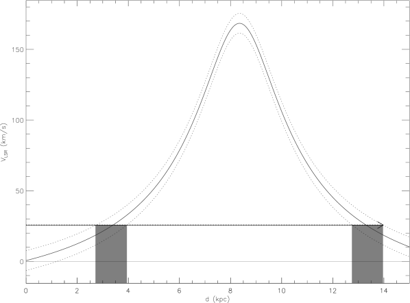
Figure 7: The flat Galactic rotation model (solid curve) of Burton (1988). The $x$-axis is the distance from the Sun along the line of sight of XTE J1810–197. The $y$-axis is the radial velocity of the gas. The dotted lines indicate the deviation from Galactic rotation of $\pm 7$ km s^-1. The arrow at $V_{\rm LSR}=25.7$ km s^-1 indicates the highest velocity H I absorption seen toward XTE J1810–197 (see Table 2). The shaded regions indicate the allowed kinematic distances from the flat rotation curve (see discussion in §§ 4.2 and 4.3 for interpretation of these figures).

References

- Becker et al. (1985) Becker, R. H., Markert, T., & Donahue, M. 1985, ApJ, 296, 461
- Brand & Blitz (1993) Brand, J., & Blitz, L. 1993, A&A, 275, 67
- Burton (1988) Burton, W. B. 1988, “The structure of our Galaxy derived from observations of H I”, in Galactic and Extragalactic Radio Astronomy (2nd edition), Berlin and New York, Springer-Verlag, 295
- Cameron et al. (2005) Cameron, P. B., et al. 2005, Nature, 434, 1112
- Camilo et al. (2006) Camilo, F., Ransom, S. R., Halpern, J. P., Reynolds, J., Helfand, D. J., Zimmerman, N., & Sarkissian, J. 2006, Nature, 442, 892
- Camilo et al. (2007a) Camilo, F., et al. 2007a, ApJ, 663, in press (astro-ph/0610685)
- Camilo et al. (2007b) Camilo, F., Reynolds, J., Johnston, S., Halpern, J. P., Ransom, S. M., & van Straten, W. 2007b, ApJ, 659, L37
- Carey et al. (2000) Carey, S. J., Feldman, P. A., Redman, R. O., Egan, M. P., MacLeod, J. M., & Price, S. D. 2000, ApJ, 543, L157
- Caswell et al. (1975) Caswell, J. L., Murray, J. D., Roger, R. S., Cole, D. J., & Cooke, D. J. 1975, A&A, 45, 239
- Corbel et al. (1997) Corbel, S., Wallyn, P., Dame, T. M., Durouchoux, P., Mahoney, W. A., Vilhu, O., & Grindlay, J. E. 1997, ApJ, 478, 624