Table-top creation of entangled multi-keV photon pairs via the Unruh effect

Abstract

Electrons moving in a strong periodic electromagnetic field (e.g., laser or undulator) may convert quantum vacuum fluctuations into pairs of entangled photons, which can be understood as a signature of the Unruh effect. Apart from verifying this striking phenomenon, the considered effect may allow the construction of a table-top source for entangled photons (“photon pair laser”) and the associated quantum-optics applications in the multi-keV regime with near-future facilities.

The striking discovery that the particle concept in quantum field theory may depend on the inertial state of the observer is one of the main lessons from the Unruh effect: The Minkowski vacuum is the ground state with respect to all stationary and inertial observers (moving with a constant velocity). However, an accelerated (i.e., non-inertial) observer generally experiences the Minkowski vacuum as an excited quantum state with a non-vanishing particle content. In case of uniform acceleration $a$, it corresponds to a thermal bath characterized by the Unruh temperature unruh

$$T_{\rm Unruh}=\frac{\hbar}{2\pi k_{\rm B}c}\,a\,.$$ (1)

Now, considering an accelerated electron, for example, there is a finite probability that a comoving (non-inertial) observer witnesses the scattering of a photon out of the thermal bath by the electron (due to its nonzero Thomson cross section). Translation of this scattering event in the accelerated frame into the (inertial) laboratory frame corresponds to the emission of pair of real photons happen . Therefore, accelerated electrons may convert (virtual) quantum vacuum fluctuations into real particle pairs chen via non-inertial scattering – which can be understood as a signature of the Unruh effect (similar to moving-mirror radiation mirror ). In a previous work habs , we studied electrons under the influence of an approximately constant electric field (corresponding to the case of uniform acceleration) and found that these signatures might be detectable for field strengths not too far below the Schwinger limit schwinger .

In the following, we shall focus on an alternative set-up (nonuniform acceleration) and consider electrons which are shot with ultra-relativistic velocities into a strong periodic (e.g., harmonic) electromagnetic field, such as a laser beam or an undulator. In the rest frame of the ultra-relativistic electrons, the (transversal) field strength is strongly boosted and thus the acceleration felt by the electrons is amplified. During each acceleration cycle, the electrons emit a small amplitude for photon pair creation and all these amplitudes may add up constructively.

In order to demonstrate the main idea, let us assume that the frequency $\omega$ (measured in the rest frame of the electrons) of the external electromagnetic field $E,B$ lies far below the electrons rest mass $m\gg\omega$ and that its normalized amplitude is much smaller than one

$$q^{2}E^{2}+q^{2}B^{2}\ll m^{2}\omega^{2}\,,$$ (2)

where $q$ is charge of electron. In the natural units $\hbar=c=\varepsilon_{0}=\mu_{0}=1$ used here, it is related to the fine-structure constant $\alpha_{\rm QED}$ via $q=\sqrt{4\pi\alpha_{\rm QED}}\approx 0.3$. In the rest frame of the electrons, their classical quivering motion induced by the external field

$$\mbox{\boldmath$r$}_{\rm cl}(t)=\mbox{\boldmath$e$}_{z}\,\frac{qE}{m\omega^{2}}\,\cos(\omega t)$$ (3)

is nonrelativistic $\mbox{\boldmath$\dot{r}$}_{\rm cl}^{2}\ll 1$ and thus the impact of the magnetic field (i.e., photon pressure) can be neglected. Furthermore, the spin of the electrons can be ignored since the spin energy $\mu_{e}B$ is much smaller than the frequency $\mu_{e}B\ll\omega$. Hence the dynamics of the electrons under the influence of the (classical plus quantum) electromagnetic field is governed by the Lagrangian

$$L(\mbox{\boldmath$\dot{r}$}_{e},\mbox{\boldmath$r$}_{e})=\frac{m}{2}\,\mbox{\boldmath$\dot{r}$}^{2}_{e}-q\mbox{\boldmath$\dot{r}$}_{e}\cdot\mbox{\boldmath$A$}(\mbox{\boldmath$r$}_{e})\,,$$ (4)

where $A$ is the vector potential in temporal gauge. Now we split the electromagnetic field $\mbox{\boldmath$A$}=\mbox{\boldmath$A$}_{\rm cl}+\mbox{\boldmath$A$}_{\rm qu}$ into a large classical part $\mbox{\boldmath$A$}_{\rm cl}$ plus small quantum fluctuations $\mbox{\boldmath$A$}_{\rm qu}$, e.g., scattered photons. Accordingly, the electron trajectory $\mbox{\boldmath$r$}_{e}=\mbox{\boldmath$r$}_{\rm cl}+\mbox{\boldmath$r$}_{\rm qu}$ is split up into the classical quivering motion $\mbox{\boldmath$r$}_{\rm cl}$ in Eq. (3) plus small quantum fluctuations $\mbox{\boldmath$r$}_{\rm qu}$ due to coupling to the quantized electromagnetic field $\mbox{\boldmath$A$}_{\rm qu}$. From the Euler-Lagrange equations

$$\frac{d}{dt}\left[m\mbox{\boldmath$\dot{r}$}_{e}-q\mbox{\boldmath$A$}(\mbox{\boldmath$r$}_{e})\right]=-q\frac{\partial}{\partial\mbox{\boldmath$r$}_{e}}\left[\mbox{\boldmath$\dot{r}$}_{e}\cdot\mbox{\boldmath$A$}(\mbox{\boldmath$r$}_{e})\right]$$ (5)

we see that the canonical momentum $\mbox{\boldmath$p$}_{e}=m\mbox{\boldmath$\dot{r}$}_{e}-q\mbox{\boldmath$A$}$ is conserved to first order $\mbox{\boldmath$p$}_{\rm qu}$ if the right-hand side vanishes. This is precisely the condition for planar Thomson scattering which is satisfied if the polarizations are orthogonal or, alternatively, for planar momenta $\mbox{\boldmath$k$}_{\rm qu},\mbox{\boldmath$k$}_{\rm cl}$

$$\mbox{\boldmath$A$}_{\rm qu}\perp\mbox{\boldmath$A$}_{\rm cl}\,\|\,\mbox{\boldmath$r$}_{\rm cl}\perp\mbox{\boldmath$r$}_{\rm qu}\,\vee\,\mbox{\boldmath$k$}_{\rm qu}\perp\mbox{\boldmath$r$}_{\rm qu}\,\|\,\mbox{\boldmath$A$}_{\rm qu}\perp\mbox{\boldmath$k$}_{\rm cl}\,.$$ (6)

In this case, we get (up to an irrelevant constant)

$$\mbox{\boldmath$\dot{r}$}_{\rm qu}=\frac{q}{m}\,\mbox{\boldmath$A$}_{\rm qu}\,.$$ (7)

Now let us consider the equations of the electromagnetic field depending on the full electron trajectory $\mbox{\boldmath$r$}_{e}(t)$

$$\mbox{\boldmath$\ddot{A}$}-\mbox{\boldmath$\nabla$}\times(\mbox{\boldmath$\nabla$}\times\mbox{\boldmath$A$})=-q\mbox{\boldmath$\dot{r}$}_{e}\delta^{3}(\mbox{\boldmath$r$}_{e}-\mbox{\boldmath$r$})\,.$$ (8)

(The longitudinal component $\mbox{\boldmath$\nabla$}\cdot\mbox{\boldmath$A$}$ is non-vanishing in temporal gauge and contains the instantaneous Coulomb field, which does not contribute to the radiation content.) Inserting the split $\mbox{\boldmath$r$}_{e}=\mbox{\boldmath$r$}_{\rm cl}+\mbox{\boldmath$r$}_{\rm qu}$ into the source term yields the classical Larmor radiation from $\mbox{\boldmath$r$}_{\rm cl}$ plus quantum corrections. There are two lowest-order corrections: variations of the electron position $\delta^{3}(\mbox{\boldmath$r$}_{\rm cl}+\mbox{\boldmath$r$}_{\rm qu}-\mbox{\boldmath$r$})$ plus the current $\mbox{\boldmath$\dot{r}$}_{\rm qu}$ due to quantum fluctuations. Since the first contribution vanishes for parallel photons $\mbox{\boldmath$k$}\|\mbox{\boldmath$k^{\prime}$}$ (the case we are mostly interested in) and does not generate polarization correlations (which will be used for detection), we shall focus on the quantum current $\mbox{\boldmath$\dot{r}$}_{\rm qu}$. Combining Eqs. (7) and (8), we obtain the effective interaction Hamiltonian for planar Thomson scattering

$$\hat{H}_{\rm eff}(t)=\frac{q^{2}}{2m}\,\mbox{\boldmath$\hat{A}$}^{2}[t,\mbox{\boldmath$r$}_{\rm cl}(t)]\,.$$ (9)

(Note that a factor of 2 is missing in habs .) The photon pairs created out of the quantum vacuum by non-inertial scattering can now be calculated via time-dependent perturbation theory yielding the two-photon amplitude

$${\mathfrak{A}}_{\mbox{\boldmath$\scriptstyle k$},\lambda,\mbox{\boldmath$\scriptstyle k^{\prime}$},\lambda^{\prime}}=\frac{q^{2}}{4m}\,\frac{\mbox{\boldmath$e$}_{\mbox{\boldmath$\scriptstyle k$},\lambda}\cdot\mbox{\boldmath$e$}_{\mbox{\boldmath$\scriptstyle k^{\prime}$},\lambda^{\prime}}}{V\sqrt{kk^{\prime}}}\,{\mathcal{F}}_{\mbox{\boldmath$\scriptstyle k$},\mbox{\boldmath$\scriptstyle k^{\prime}$}}\,,$$ (10)

where $V$ is the quantization volume and $\mbox{\boldmath$e$}_{\mbox{\boldmath$\scriptstyle k$},\lambda}$, $\mbox{\boldmath$e$}_{\mbox{\boldmath$\scriptstyle k^{\prime}$},\lambda^{\prime}}$ denote the (linear) polarization vectors of the two created photons with wave-numbers $k$ and $k^{\prime}$, respectively. The remaining time integral,

$${\mathcal{F}}_{\mbox{\boldmath$\scriptstyle k$},\mbox{\boldmath$\scriptstyle k^{\prime}$}}=i\int dt\,\exp\left\{i(k+k^{\prime})t-i(\mbox{\boldmath$k$}+\mbox{\boldmath$k^{\prime}$})\cdot\mbox{\boldmath$r$}_{\rm cl}(t)\right\}\,,$$ (11)

can be Taylor expanded for small oscillation amplitudes

$${\mathcal{F}}_{\mbox{\boldmath$\scriptstyle k$},\mbox{\boldmath$\scriptstyle k^{\prime}$}}\approx\int dt\,e^{i(k+k^{\prime})t}(\mbox{\boldmath$k$}+\mbox{\boldmath$k^{\prime}$})\cdot\mbox{\boldmath$r$}_{\rm cl}(t)\,,$$ (12)

and just yields the Fourier transform of the quivering motion $(\mbox{\boldmath$k$}+\mbox{\boldmath$k^{\prime}$})\cdot\mbox{\boldmath$\tilde{r}$}_{\rm cl}(k+k^{\prime})$ evaluated at a frequency of $k+k^{\prime}$ and projected onto $\mbox{\boldmath$k$}+\mbox{\boldmath$k^{\prime}$}$. The resonance condition (energy conservation) reads $k+k^{\prime}=\omega$ and at resonance $k+k^{\prime}=\omega$, the amplitude yields

$${\mathfrak{A}}_{\mbox{\boldmath$\scriptstyle k$},\lambda,\mbox{\boldmath$\scriptstyle k^{\prime}$},\lambda^{\prime}}=\frac{q^{3}E}{8m^{2}}\,\frac{\mbox{\boldmath$e$}_{\mbox{\boldmath$\scriptstyle k$},\lambda}\cdot\mbox{\boldmath$e$}_{\mbox{\boldmath$\scriptstyle k^{\prime}$},\lambda^{\prime}}}{\omega^{3}V}\,\frac{k_{z}+k_{z}^{\prime}}{\sqrt{kk^{\prime}}}\,\omega T\,,$$ (13)

where $\omega T$ counts the number of laser cycles experienced by the electrons. The probability of emitting a pair of photons in resonance band $k+k^{\prime}=\omega\pm{\cal O}(1/T)$ can be estimated via $\sum_{\lambda,\lambda^{\prime}}(\mbox{\boldmath$e$}_{\mbox{\boldmath$\scriptstyle k$},\lambda}\cdot\mbox{\boldmath$e$}_{\mbox{\boldmath$\scriptstyle k^{\prime}$},\lambda^{\prime}})^{2}=1+(\mbox{\boldmath$e$}_{\mbox{\boldmath$\scriptstyle k$}}\cdot\mbox{\boldmath$e$}_{\mbox{\boldmath$\scriptstyle k^{\prime}$}})^{2}\geq 1$

$${\mathfrak{P}}_{\rm Unruh}>\frac{\alpha_{\rm QED}^{2}}{(4\pi)^{2}}\left[\frac{E}{E_{S}}\right]^{2}\times{\cal O}\left(\frac{\omega T}{30}\right)\ll 1\,,$$ (14)

where $E_{S}=m^{2}/q$ denotes the Schwinger limit schwinger and the exact pre-factor depends on the pulse shape etc. .

Of course, the electron does not just act as a scatterer, but also possesses a charge – and, as every accelerated charge, emits Larmor radiation. This classical radiation corresponds to a coherent state and can fully be described by the associated one-photon amplitude

$$\alpha_{\mbox{\boldmath$\scriptstyle k$},\lambda}=q\int dt\,\frac{\mbox{\boldmath$e$}_{\mbox{\boldmath$\scriptstyle k$},\lambda}\cdot\mbox{\boldmath$\dot{r}$}_{\rm cl}(t)}{\sqrt{2Vk}}\,\exp\{ikt-i\mbox{\boldmath$k$}\cdot\mbox{\boldmath$r$}_{\rm cl}(t)\}\,.$$ (15)

From the scalar product $\mbox{\boldmath$e$}_{\mbox{\boldmath$\scriptstyle k$},\lambda}\cdot\mbox{\boldmath$\dot{r}$}_{\rm cl}$, one may read off the well-known blind spot and the fixed polarization. Similarly to the above estimate (14), the one-photon probability of this classical counterpart yields

$${\mathfrak{P}}_{\rm Larmor}^{(1)}=\frac{\alpha_{\rm QED}}{2\pi}\left[\frac{qE}{m\omega}\right]^{2}\times{\cal O}\left(\frac{\omega T}{3}\right)\,.$$ (16)

In view of $\omega\ll m$, the total classical probability above exceeds the probability ${\mathfrak{P}}_{\rm Unruh}$ of quantum radiation. However, as one may infer from Eq. (15), the classical resonance condition reads $k=\omega$, i.e., the Larmor photons are predominantly monochromatic (in the electron frame). In contrast, the photon pairs created via the Unruh effect occur at different frequencies, as long as they satisfy $k+k^{\prime}=\omega$, i.e., these pairs are correlated in energy and polarization. (Whereas Larmor radiation has a fixed polarization and a blind spot in $z$-direction.) Note that the ratio of the probabilities in Eqs. (14) and (16) is roughly independent of the field strength $E$ given by

$$\frac{{\mathfrak{P}}_{\rm Unruh}}{{\mathfrak{P}}_{\rm Larmor}^{(1)}}={\cal O}\left(\frac{\alpha_{\rm QED}}{80\pi}\,\frac{\omega^{2}}{m^{2}}\right)\,.$$ (17)

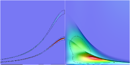
Figure 1: $E$-$\vartheta$ plot of the one-photon probability of classical (Larmor, left half of image) and quantum (Unruh, right) radiation in the laboratory frame. An electron with a boost factor of $\gamma=300$ hits a counter-propagating optical Gaussian laser pulse with an intensity around $10^{18}\rm W/cm^{2}$ and a half-width of 100 cycles. The photon energy $E$ ranges from zero (bottom) to 2 MeV (top) and $\vartheta$ varies from zero (middle) to 1/100 (left and right boundary). In the chosen color coding (not the same in the two images), red indicates a large and dark blue a vanishing probability. The black iso-lines denote the same values in both pictures and show that the quantum radiation dominates in certain phase space regions (which could be extracted with apertures and energy filters). For example, cutting out a small cone around the blind spot (at $\vartheta=1/300$ in the left picture) drastically increases the Unruh-Larmor ratio (17). As one may infer from the visibility of the second harmonic, relativistic effects already start to play a role for this set of parameters ($\mbox{\boldmath$\dot{r}$}_{\rm cl}^{2}\approx 1/9$). Therefore, we numerically calculated the full electron trajectory (including the impact of the magnetic field) and inserted it into Eqs. (10), (11), and (15), respectively.

Let us insert a set of parameters which are potentially realizable with present or near-future technology design . Assuming an optical laser beam with a photon energy of 2.5 eV (in the laboratory frame) and a boost factor of $\gamma=300$, the photon energy in rest frame of the electrons $\omega=1.5\,\rm keV$ is still much smaller than the electron mass. With a laser intensity of order $10^{18}\,\rm W/cm^{2}$ in the laboratory frame, the electric field $E$ lies a factor of $1000$ below the Schwinger limit $E_{S}$ in the rest frame of the electrons and their transversal quivering motion $\mbox{\boldmath$\dot{r}$}_{\rm cl}^{2}\approx 1/9$ is still approximately nonrelativistic. After 100 laser cycles (half-width of Gaussian pulse), we obtain a two-photon probability of order $10^{-11}$ frome one electron. Depending on their direction, the sum of the energies of the created photons in the laboratory frame is then around 500 keV . The total probability for the competing classical counterpart (Larmor radiation) is much higher ${\cal O}(10^{-2})$. Fortunately, the monochromatic character (rest frame of electrons) of the Larmor radiation (which just corresponds to Thomson scattering of the laser photons) in our set-up ensures that the phase-space regions of the two effects are very different. In the laboratory frame, the phase space is quite distorted after the boost, see Fig. 1, but it is (at least in principle) still possible to discriminate the two effects via suitable apertures and energy filters etc.

So far, we considered the case of single electrons only. For many electrons, their space-time distribution and the resulting spatial interference becomes important (in addition to the temporal interference, which yields the resonance conditions $k=\omega$ and $k+k^{\prime}=\omega$, respectively). For both, classical and quantum radiation, one should distinguish two major limiting cases: incoherent or coherent superposition. If the electrons are randomly distributed and their typical distance is much larger than $1/\omega$, we have an incoherent superposition (addition of probabilities). For example, sending such a pulse of $N_{e}=10^{9}$ independent electrons into a laser beam with the values discussed above, we obtain around one Unruh event in hundred shots. Of course, a coherent superposition (constructive interference of amplitudes) would be much more effective. One possibility to achieve the necessary phase coherence could be to confine all the electrons to within half a wavelength $\pi/\omega$. For optical lasers, this is probably hard to do. However, in an other system, an analogous spatial phase coherence has been achieved already: In undulators for free-electron lasers (FEL) based on self-amplification of spontaneous emission (SASE), the original electron pulse is split up into many nearly equidistant micro-bunches via the back-reaction of the Larmor radiation. These micro-bunches contain a significant fraction of the total number of electrons and occur at distances equal to half the undulator period (in the frame of the electrons). Therefore, the amplitudes generated by the zig-zag motion of these micro-bunches interfere constructively in forward (i.e., electron beam) direction – leading to the amplification of Larmor radiation (in the ideal case $\propto N_{e}^{2}$ instead of $\propto N_{e}$). Comparing Eqs. (11) and (15), we see that the quantum (two-photon) amplitudes (13) do also interfere constructively if both photons (with $k+k^{\prime}=\omega$) are emitted in forward direction.

Let us estimate the order of magnitude for a realistic set of parameters envisioned for near future facilities design . Sending a pulse containing $6\times 10^{9}$ electrons with a boost factor of $\gamma=4000$ into an undulator with a period of order ten millimeters, the frequency in the electron frame is $\omega={\cal O}(1\,\rm eV)$. For an undulator, the $K$-factor plays the role of the normalized amplitude of the laser in Eq. (2) and is assumed to be below one. After around 100 periods (undulator length of order one meter), we obtain a single-electron Larmor probability (16) on the percent level. However, the expected yield of $>10^{12}$ photons already indicates that the $6\times 10^{9}$ electrons do not radiate independently but interfere constructively. Unfortunately, not all electrons of the pulse will behave coherently, the effective fraction of electrons which are in phase is given by the bunching factor, which is also assumed to be on the percent level. Still, calculating the Unruh-Larmor ratio ${\mathfrak{P}}_{\rm Unruh}/{\mathfrak{P}}_{\rm Larmor}^{(1)}={\cal O}(10^{-14})$, we would again expect one Unruh pair in around one hundred shots .

By adding up the amplitudes generated by many electrons coherently, it might even be possible to reach the non-perturbative regime, where multi-photon effects become important. In this regime, there is a crucial difference between quantum and classical radiation: Classical radiation can be described by a coherent state

$$\left|\alpha\right>=\exp\{\alpha\hat{a}^{\dagger}-\alpha^{*}\hat{a}\}\left|0\right>\,.$$ (18)

In this case, the photon number $\left<\alpha\right|\hat{n}\left|\alpha\right>=|\alpha|^{2}$ scales quadratically with the number of electrons $\alpha\propto N_{e}$ (constructive interference). Quantum radiation, on the other hand, corresponds to a (multi-mode) squeezed state

$$\left|\xi\right>=\exp\left\{\xi\hat{a}_{1}^{\dagger}\hat{a}_{2}^{\dagger}-\xi^{*}\hat{a}_{1}\hat{a}_{2}\right\}\left|0\right>\,,$$ (19)

where we consider two modes $\hat{a}_{1}$ and $\hat{a}_{2}$ for simplicity. For small amplitudes $\xi\ll 1$, the photon number $\left<\xi\right|\hat{n}_{1}\left|\xi\right>=\sinh^{2}(|\xi|)$ also scales quadratically with the number of electrons $\xi\propto N_{e}$, but after a certain threshold $\xi={\cal O}(1)$ is reached, it grows exponentially . Ignoring all geometrical factors, the threshold can be estimated from Eq. (13): after passing

$$N_{e}={\cal O}\left(\alpha_{\rm QED}^{-1}\frac{E_{S}}{E}\right)$$ (20)

electrons (in the oscillating micro-bunches), the two-photon wave-packets start to grow exponentially (until their growth is limited by back-reaction etc.). Reaching this threshold is a quite ambitious goal, but may become within reach with the next generation of free-electron lasers (FEL).

The signatures of the Unruh effect discussed above bear strong similarities to (spontaneous) parametric down-conversion known from quantum optics: The external periodic electromagnetic field corresponds to the pump beam and the electrons are analogous to the nonlinear dielectric medium. In both cases, the scattering properties (refractive index) of the medium are varied periodically (frequency $\omega$) by the pump beam and thereby the quantum vacuum fluctuations of the electromagnetic field are converted into a pair of entangled photons (signal and idler) whose energies add up to the pump frequency $k+k^{\prime}=\omega$. In quantum optics, this mechanism is the main source for entangled photon pairs which have a wide range of applications including concepts known from quantum information theory (e.g., tests of Bell’s inequality, quantum cryptography, or teleportation), two-photon interferometry, photonic Fock states (i.e., states with a well-defined photon number, which could be used for counting excitations, for example), heralded photon emission, and coincidence experiments etc. Since the quantum radiation discussed here consists of entangled photon pairs with much higher energies (which are more robust against some disturbances and offer higher interaction rates), it may allow the transfer of these quantum-optics applications into the multi-keV regime (see also nuclear ).

R. S. and G. S. were supported by the Emmy-Noether Programme of the German Research Foundation (DFG, grant # SCHU 1557/1-2). The authors acknowledge support by the DFG cluster of excellence MAP and fruitful discussions with F. Grüner, U. Schramm, J. Schreiber, and P. Thirolf.

^∗schuetz@theory.phy.tu-dresden.de

References

- (1) W. G. Unruh, Phys. Rev. D 14, 870 (1976).
- (2) W. G. Unruh and R. M. Wald, Phys. Rev. D 29, 1047 (1984).
- (3) The important point that the photons are always created in pairs has not been taken into account adequately in previous works on this topic, such as P. Chen and T. Tajima, Phys. Rev. Lett. 83, 256 (1999).
- (4) G. T. Moore, J. Math. Phys. 11, 2679 (1970).
- (5) R. Schützhold, G. Schaller, and D. Habs, Phys. Rev. Lett. 97, 121302 (2006).
- (6) J. Schwinger, Phys. Rev. 82, 664 (1951); see also E. Gerstner, Nature 446, 16 (2007).
- (7) F. Grüner et al, Appl. Phys. B 86, (R) 431 (2007).
- (8) I. Freund and B. F. Levine, Phys. Rev. Lett. 23, 854 (1969); P. Eisenberger, S.L. McCall, Phys. Rev. Lett. 26, 684 (1971); Y. Yoda et al, J. Synchroton Rad. 5, 980 (1998); B. Adams et al, ibid. 7, 81 (2000).
- (9) T. J. Bürvenich, J. Evers, and C. H. Keitel, Phys. Rev. Lett. 96, 142501 (2006).