Enhancing SPH using Moving Least-Squares and Radial Basis Functions

Abstract

In this paper we consider two sources of enhancement for the meshfree Lagrangian particle method smoothed particle hydrodynamics (SPH) by improving the accuracy of the particle approximation. Namely, we will consider shape functions constructed using: moving least-squares approximation (MLS); radial basis functions (RBF). Using MLS approximation is appealing because polynomial consistency of the particle approximation can be enforced. RBFs further appeal as they allow one to dispense with the smoothing-length – the parameter in the SPH method which governs the number of particles within the support of the shape function. Currently, only ad hoc methods for choosing the smoothing-length exist. We ensure that any enhancement retains the conservative and meshfree nature of SPH. In doing so, we derive a new set of variationally-consistent hydrodynamic equations. Finally, we demonstrate the performance of the new equations on the Sod shock tube problem.

1 Introduction

Smoothed particle hydrodynamics (SPH) is a meshfree Lagrangian particle method primarily used for solving problems in solid and fluid mechanics (see rab_Monaghan05 for a recent comprehensive review). Some of the attractive characteristics that SPH possesses include: the ability to handle problems with large deformation, free surfaces and complex geometries; truly meshfree nature (no background mesh required); exact conservation of momenta and total energy. On the other hand, SPH suffers from several drawbacks: an instability in tension; difficulty in enforcing essential boundary conditions; fundamentally based on inaccurate kernel approximation techniques. This paper addresses the last of these deficiencies by suggesting improved particle approximation procedures. Previous contributions in this direction (reviewed in rab_Belytschko96 ) have focused on corrections of the existing SPH particle approximation (or its derivatives) by enforcing polynomial consistency. As a consequence, the conservation of relevant physical quantities by the discrete equations is usually lost.

The outline of the paper is as follows. In the next section we review how SPH equations for the non-dissipative motion of a fluid can be derived. In essence this amounts to a discretization of the Euler equations:

$$\frac{\mathrm{d}\rho}{\mathrm{d}t}=-\rho\nabla\cdot v,\qquad\frac{\mathrm{d}v}{\mathrm{d}t}=-\frac{1}{\rho}\nabla P,\qquad\frac{\mathrm{d}e}{\mathrm{d}t}=-\frac{P}{\rho}\nabla\cdot v,$$ (1)

where $\frac{\mathrm{d}}{\mathrm{d}t}$ is the total derivative, $\rho$, $v$, $e$ and $P$ are the density, velocity, thermal energy per unit mass and pressure, respectively. The derivation is such that important conservation properties are satisfied by the discrete equations. Within the same section we derive a new set of variationally-consistent hydrodynamic equations based on improved particle approximation. In Sect. 3 we construct specific examples – based on moving least-squares approximation and radial basis functions – to complete the newly derived equations. The paper finishes with Sect. 4 where we demonstrate the performance of the new methods on the Sod shock tube problem rab_Sod78 and make some concluding remarks.

To close this section, we briefly review the SPH particle approximation technique on which the SPH method is fundamentally based and which we purport to be requiring improvement. From a set of scattered particles $\{x_{1},\ldots,x_{N}\}\subset{\mathord{\rm I\mkern-3.6muR}}^{d}$, SPH particle approximation is achieved using

$$Sf(x)=\sum_{j=1}^{N}f(x_{j})\frac{m_{j}}{\rho_{j}}W(|x-x_{j}|,h),$$ (2)

where $m_{j}$ and $\rho_{j}$ denotes the mass and density of the $j$th particle, respectively. The function $W$ is a normalised kernel function which approximates the $\delta$-distribution as the smoothing-length, $h$, tends to zero. The function $\frac{m_{j}}{\rho_{j}}W(|x-x_{j}|,h)$ is called an SPH shape function and the most popular choice for $W$ is a compactly supported cubic spline kernel with support $2h$. The parameter $h$ governs the extent to which contributions from neighbouring particles are allowed to smooth the approximation to the underlying function $f$. Allowing a spatiotemporally varying smoothing-length increases the accuracy of an SPH simulation considerably. There are a selection of ad hoc techniques available to accomplish this, although often terms arising from the variation in $h$ are neglected in the SPH method. The approximating power of the SPH particle approximation is perceived to be poor. The SPH shape functions fail to provide a partition of unity so that even the constant function is not represented exactly. There is currently no approximation theory available for SPH particle approximation when the particles are in general positions. The result of a shock tube simulation using the SPH equations derived in Sect. 2 is shown in Fig. 1 (see Sect. 4 for the precise details of the simulation).

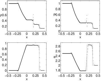
Figure 1: Shock tube simulation (t=$0.2$) using SPH.

The difficulty that SPH has at the contact discontinuity ($x\approx 0.2$) and the head of the rarefaction wave ($x\approx-0.25$) is attributed to a combination of the approximation (2) and the variable smoothing-length not being self-consistently incorporated.

2 Variationally-Consistent Hydrodynamic Equations

It is well known (see rab_Monaghan05 and the references cited therein) that the most common SPH equations for the non-dissipative motion of a fluid can be derived using the Lagrangian for hydrodynamics and a variational principle. In this section we review this procedure for a particular formulation of SPH before deriving a general set of variationally-consistent hydrodynamic equations.

The aforementioned Lagrangian is a particular functional of the dynamical coordinates: $L(x,v)=\int\rho(v^{2}/2-e)\,\mathrm{d}x$, where $x$ is the position, $v$ is the velocity, $\rho$ is the density, $e$ is the thermal energy per unit mass and the integral is over the volume being discretized. Given $N$ particles $\{x_{1}\ldots,x_{N}\}\subset{\mathord{\rm I\mkern-3.6muR}}^{d}$, the SPH discretization of the Lagrangian, also denoted by $L$, is given by

$$L=\sum_{j=1}^{N}m_{j}\Bigl{(}\frac{v_{j}^{2}}{2}-e_{j}\Bigr{)},$$ (3)

where $m_{j}$ has replaced $\rho_{j}V_{j}$ to denote particle mass (assumed to be constant), and $V_{j}$ is a volume associated with each particle. Self-evidently, the notation $f_{j}$ is used to denote the function $f$ evaluated at the $j$th particle.

The Euler-Lagrange equations give rise to SPH equations of motion provided each quantity in (3) can be written directly as a function of the particle coordinates. By setting $f=\rho$ in (2) and evaluating at $x_{j}$, we can obtain an expression for $\rho_{j}$ directly as a function of the particle coordinates. Therefore, because we assume that $e_{j}=e_{j}(\rho_{j})$, the Euler–Lagrange equations are amenable. Furthermore, in using this approach, conservation of momenta and total energy are guaranteed via Noether’s symmetry theorem. However, when we consider improved particle approximation, the corresponding expression for density depends on the particle coordinates in an implicit manner, so that the Euler–Lagrange equations are not directly amenable. To circumvent this difficulty, one can use the principle of stationary action directly to obtain SPH equations of motion – the action,

$$S=\int L\,\mathrm{d}t,$$

being the time integral of $L$. The principle of stationary action demands that the action is invariant with respect to small changes in the particle coordinates (i.e., $\delta S=0$). The Euler–Lagrange equations are a consequence of this variational principle. In rab_Monaghan05 it is shown that if an expression for the time rate of change of $\rho_{j}$ is available, then, omitting the detail, this variational principle gives rise to SPH equations of motion.

To obtain an expression for the time rate of change of density we can discretize the first equation of (1) using (2) by collocation. By assuming that the SPH shape functions form a partition of unity we commit error but are able to artificially provide the discretization with invariance to a constant shift in velocity (Galilean invariance):

$$\frac{\mathrm{d}\rho_{i}}{\mathrm{d}t}=-\rho_{i}\sum_{j=1}^{N}\frac{m_{j}}{\rho_{j}}(v_{j}-v_{i})\cdot\nabla_{i}W(|x_{i}-x_{j}|,h_{i}),\qquad\text{$i=1,\ldots,N$,}$$ (4)

where $\nabla_{i}$ is the gradient with respect to the coordinates of the $i$th particle. The equations of motion that are variationally-consistent with (4) are

$$\frac{\mathrm{d}v_{i}}{\mathrm{d}t}=-\frac{1}{\rho_{i}}\sum_{j=1}^{N}\frac{m_{j}}{\rho_{j}}\Bigl{(}P_{i}\nabla_{i}W(|x_{i}-x_{j}|,h_{i})+P_{j}\nabla_{i}W(|x_{i}-x_{j}|,h_{j})\Bigr{)},$$ (5)

for $i=1,\ldots,N$, where $P_{i}$ denotes the pressure of the $i$th particle (provided via a given equation of state). Using the first law of thermodynamics, the equation for the rate of change of thermal energy is given by

$$\frac{\mathrm{d}e_{i}}{\mathrm{d}t}=\frac{P_{i}}{\rho_{i}^{2}}\frac{\mathrm{d}\rho_{i}}{\mathrm{d}t},\qquad\text{$i=1,\ldots,N$.}$$ (6)

As already noted, a beneficial consequence of using the Euler–Lagrange equations is that one automatically preserves, in the discrete equations, fundamental conservation properties of the original system (1). Since we have not done this, conservation properties are not necessarily guaranteed by our discrete equations (4)–(6). However, certain features of the discretization (4) give us conservation. Indeed, by virtue of (4) being Galilean invariant, one conserves linear momentum and total energy (assuming perfect time integration). Remember that Galilean invariance was installed under the erroneous assumption that the SPH shape functions provide a partition of unity. Angular momentum is also explicitly conserved by this formulation due to $W$ being symmetric.

Now, we propose to enhance SPH by improving the particle approximation (2). Suppose we have constructed shape functions $\phi_{j}$ that provide at least a partition of unity. With these shape functions we form a quasi-interpolant:

$$Sf=\sum_{j=1}^{N}f(x_{j})\phi_{j},$$ (7)

which we implicitly assume provides superior approximation quality than that provided by (2). We defer particular choices for $\phi_{j}$ until the next section. The discretization of the continuity equation now reads

$$\frac{\mathrm{d}\rho_{i}}{\mathrm{d}t}=-\rho_{i}\sum_{j=1}^{N}(v_{j}-v_{i})\cdot\nabla\phi_{j}(x_{i}),\qquad\text{$i=1,\ldots,N$,}$$ (8)

where, this time, we have supplied genuine Galilean invariance, without committing an error, using the partition of unity property of $\phi_{j}$. As before, the principle of stationary action provides the equations of motion and conservation properties of the resultant equations reflect properties present in the discrete continuity equation (8).

To obtain (3), two assumptions were made. Firstly, the SPH shape functions were assumed to form a sufficiently good partition of unity. Secondly, it was assumed that the kernel approximation $\int fW(|\cdot-x_{j}|,h)\,\mathrm{d}x\approx f(x_{j})$, was valid. For our general shape functions the first of these assumptions is manifestly true. The analogous assumption we make to replace the second is that the error induced by the approximations

$$\int f\phi_{j}\,\mathrm{d}x\approx f_{j}\int\phi_{j}\,\mathrm{d}x\approx f_{j}V_{j},\qquad\text{$j=1,\ldots,N$},$$ (9)

is negligible. With the assumption (9), the approximate Lagrangian associated with $\phi_{j}$ is identical in form to (3). Neglecting the details once again, which can be recovered from rab_Monaghan05 , the equations of motion variationally-consistent with (8) are

$$\frac{\mathrm{d}v_{i}}{\mathrm{d}t}=\frac{1}{m_{i}}\sum_{j=1}^{N}\frac{m_{j}}{\rho_{j}}P_{j}\nabla\phi_{i}(x_{j}),\qquad\text{$i=1,\ldots,N$,}$$ (10)

The equations (6), (8) and (10) constitute a new set of variationally-consistent hydrodynamic equations. They give rise to the formulation of SPH derived earlier under the transformation $\phi_{j}(x_{i})\mapsto\frac{m_{j}}{\rho_{j}}W(|x_{i}-x_{j}|,h_{i})$. The equations of motion (10) appear in rab_Dilts00 but along side variationally-inconsistent companion equations. The authors advocate using a variationally-consistent set of equation because evidence from the SPH literature (e.g., rab_Bonet99 ; rab_Marri03 ) suggests that not doing so can lead to poor numerical results.

Linear momentum and total energy are conserved by the new equations, and this can be verified immediately using the partition of unity property of $\phi_{j}$. The $\phi_{j}$ will not be symmetric. However, if it is also assumed that the shape functions reproduce linear polynomials, namely, $\sum x_{j}\phi_{j}(x)=x$, then it is simple to verify that angular momentum is also explicitly conserved.

3 Moving Least-Squares and Radial Basis Functions

In this section we construct quasi-interpolants of the form (7). In doing so we furnish our newly derived hydrodynamic equations (6), (8) and (10) with several examples.

Moving least-squares (MLS).

The preferred construction for MLS shape functions, the so-called Backus–Gilbert approach rab_Bos89 , seeks a quasi-interpolant of the form (7) such that:

• $Sp=p$ for all polynomials $p$ of some fixed degree;

• $\phi_{j}(x)$, $j=1,\ldots,N$, minimise the quadratic form $\sum\phi_{j}^{2}(x)\Bigl{[}w\Bigl{(}\frac{|x-x_{j}|}{h}\Bigr{)}\Bigr{]}^{-1},$

where $w$ is a fixed weight function. If $w$ is continuous, compactly supported and positive on its support, this quadratic minimisation problem admits a unique solution. Assuming $f$ has sufficient smoothness, the order of convergence of the MLS approximation (7) directly reflects the degree of polynomial reproduced rab_Wendland01 .

The use of MLS approximation in an SPH context has been considered before. Indeed, Belytschko et al. rab_Belytschko96 have shown that correcting the SPH particle approximation up to linear polynomials is equivalent to an MLS approximation with $w(|\cdot-x_{j}|/h)=W(|\cdot-x_{j}|,h)$. There is no particular reason to base the MLS approximation on an SPH kernel. We find that MLS approximations based on Wendland functions rab_Wendland95 , which have half the natural support of a typical SPH kernel, produce results which are less noisy. Dilts rab_Dilts99 ; rab_Dilts00 employs MLS approximation too. Indeed, in rab_Dilts99 , Dilts makes an astute observation that addresses an inconsistency that arises due to (9) – we have the equations

$$\frac{\mathrm{d}V_{i}}{\mathrm{d}t}=V_{i}\sum_{j=1}^{N}(v_{j}-v_{i})\cdot\nabla\phi_{j}(x_{i})\qquad\text{and}\qquad\frac{\mathrm{d}V_{i}}{\mathrm{d}t}\approx\frac{\mathrm{d}}{\mathrm{d}t}\biggl{(}\int\phi_{i}(x)\,\mathrm{d}x\biggr{)}.$$

Dilts shows that if $h_{i}$ is evolved according to $h_{i}\propto V_{i}^{1/d}$ then there is agreement between the right-hand sides of these equations when a one-point quadrature of $\int\phi_{i}\,\mathrm{d}x$ is employed. Thus, providing some theoretical justification for choosing this particular variable smoothing-length over other possible choices.

Radial basis functions (RBFs).

To construct an RBF interpolant to an unknown function $f$ on $x_{1},\ldots,x_{N}$, one produces a function of the form

$$If=\sum_{j=1}^{N}\lambda_{j}\psi(|\cdot-x_{j}|),$$ (11)

where the $\lambda_{j}$ are found by solving the linear system $If(x_{i})=f(x_{i})$, $i=1,\ldots,N$. The radial basis function, $\psi$, is a pre-specified univariate function chosen to guarantee the solvability of this system. Depending on the choice of $\psi$, a low degree polynomial is sometimes added to (11) to ensure solvability, with the additional degrees of freedom taken up in a natural way. This is the case with the polyharmonic splines, which are defined, for $m>d/2$, by $\psi(|x|)=|x|^{2m-d}\log{|x|}$ if $d$ is even and $\psi(|x|)=|x|^{2m-d}$ otherwise, and a polynomial of degree $m-1$ is added. The choice $m\geq 2$ ensures the RBF interpolant reproduces linear polynomials as required for angular momentum to be conserved by the equations of motion. As with MLS approximation, one has certain strong assurances regarding the quality of the approximation induced by the RBF interpolant (e.g. rab_Brownlee04 for the case of polyharmonic splines).

In its present form (11), the RBF interpolant is not directly amenable. One possibility is to rewrite the interpolant in cardinal form so that it coincides with (7). This naively constitutes much greater computational effort. However, there are several strategies for constructing approximate cardinal RBF shape functions (e.g. rab_Brown05 ) and fast evaluation techniques (e.g. rab_Beatson97 ) which reduce this work significantly. The perception of large computational effort is an attributing factor as to why RBFs have not been considered within an SPH context previously. Specifically for polyharmonic splines, another possibility is to construct shape functions based on discrete $m$-iterated Laplacians of $\psi$. This is sensible because the continuous iterated Laplacian, when applied $\psi$, results in the $\delta$-distribution (up to a constant). This is precisely the approach we take in Sect. 4 where we employ cubic B-spline shape functions for one of our numerical examples. The cubic B-splines are discrete bi-Laplacians of the shifts of $|\cdot|^{3}$, and they gladly reproduce linear polynomials.

In addition to superior approximation properties, using globally supported RBF shape functions has a distinct advantage. One has dispensed with the smoothing-length entirely. Duely, issues regarding how to correctly vary and self-consistently incorporate the smoothing-length vanish. Instead, a natural ‘support’ is generated related to the relative clustering of particles.

4 Numerical Results

In this section we demonstrate the performance of the scheme (6), (8) and (10) using both MLS and RBF shape functions. The test we have selected has become a standard one-dimensional numerical test in compressible fluid flow – the Sod shock tube rab_Sod78 . The problem consists of two regions of ideal gas, one with a higher pressure and density than the other, initially at rest and separated by a diaphragm. The diaphragm is instantaneously removed and the gases allowed to flow resulting in a rarefaction wave, contact discontinuity and shock. We set up $450$ equal mass particles in $[-0.5,0.5]$. The gas occupying the left-hand and right-hand sides of the domain are given initial conditions $(P_{L},\rho_{L},v_{L})=(1.0,1.0,0.0)$ and $(P_{R},\rho_{R},v_{R})=(0.1,0.125,0.0)$, respectively. The initial condition is not smoothed.

With regards to implementation, artificial viscosity is included to prevent the development of unphysical oscillations. The form of the artificial viscosity mimics that of the most popular SPH artificial viscosity and is applied with a switch which reduces the magnitude of the viscosity by a half away from the shock. A switch is also used to administer an artificial thermal conductivity term, also modelled in SPH. Details of both dissipative terms and their respective switches can be accessed through rab_Monaghan05 . Finally, we integrate, using a predictor–corrector method, the equivalent hydrodynamic equations

$$\frac{\mathrm{d}V_{i}}{\mathrm{d}t}=V_{i}\sum_{j=1}^{N}(v_{j}-v_{i})\cdot\nabla\phi_{j}(x_{i}),$$ (12)

$$\frac{\mathrm{d}v_{i}}{\mathrm{d}t}=\frac{1}{m_{i}}\sum_{j=1}^{N}V_{j}P_{j}\nabla\phi_{i}(x_{j}),\qquad\frac{\mathrm{d}e_{i}}{\mathrm{d}t}=-\frac{P_{i}}{m_{i}}\frac{\mathrm{d}V_{i}}{\mathrm{d}t},$$

together with $\frac{\mathrm{d}x_{i}}{\mathrm{d}t}=v_{i}$, to move the particles. To address the consistency issue regarding particle volume mentioned earlier – which is partially resolved by evolving $h$ in a particular way when using MLS approximation – we periodically update the particle volume predicted by (12) with $\int\phi_{i}\,\mathrm{d}x$ if there is significant difference between these two quantities. To be more specific, the particle volume $V_{i}$ is updated if $|V_{i}-\int\phi_{i}\,\mathrm{d}x|/V_{i}\geq 1.0\times 10^{-3}$.

We first ran a simulation with linearly complete MLS shape functions. The underlying univariate function, $w$, was selected to be a Wendland function with $C^{4}$-smoothness. The smoothing-length was evolved by taking a time derivative of the relationship $h_{i}\propto V_{i}$ and integrating it alongside the other equations, the constant of proportionality was chosen to be $2.0$. The result is shown in Fig. 2.

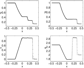
Figure 2: Shock tube simulation (t=$0.2$) using linearly complete MLS shape functions.

The agreement with the analytical solution (solid line) is excellent, especially around the contact discontinuity and the head of the rarefaction wave. Next, we constructed RBF shape functions. As we mentioned in Sect. 3, for this one-dimensional problem we employ cubic B-spline because they constitute discrete bi-Laplacians of the shifts of the globally supported basis function, $\psi=|\cdot|^{3}$. The result of this simulation is shown in Fig. 3.

Figure 3: Shock tube simulation (t=$0.2$) using cubic B-spline shape functions.

Again, the agreement with the analytical solution is excellent.

In the introduction an SPH simulation of the shock tube was displayed (Fig. 1). There, we integrated (4)–(6) and $h$ was updated by taking a time derivative of the relationship $h_{i}=2.0m_{i}/\rho_{i}$. To keep the comparison fair, the same initial condition, particle setup and dissipative terms were used. As previously noted, this formulation of SPH performs poorly on this problem, especially around the contact discontinuity. Furthermore, we find that this formulation of SPH does not converge in the $L_{\infty}$-norm for this problem. At a fixed time ($t=0.2$), plotting number of particles, $N$, versus $L_{\infty}$-error in pressure, in the region of the computational domain where the solution is smooth reveals an approximation order of around $2/3$, attributed to the low regularity of the analytical solution, for the MLS and RBF methods, whereas our SPH simulation shows no convergence. This is not to say that SPH can not perform well on this problem. Indeed, Price rab_Price04 shows that, for a formulation of SPH where density is calculated via summation and variable smoothing-length terms correctly incorporated, the simulation does exhibit convergence in pressure. The SPH formulation we have used is fair for comparison with the MLS and RBF methods since they all share a common derivation. In particular, we are integrating the continuity equation in each case.

To conclude, we have proposed a new set of discrete conservative variationally-consistent hydrodynamic equations based on a partition of unity. These equations, when actualised with MLS and RBF shape functions, outperform the SPH method on the shock tube problem. Further experimentation and numerical analysis of the new methods is a goal for future work.

Acknowledgements.

The first author would like to acknowledge Joe Monaghan, whose captivating lectures at the XIth NA Summer School held in Durham in July 2004 provided much inspiration for this work. Similarly, the first author would like to thank Daniel Price for his useful discussions, helpful suggestions and hospitality received during a visit to Exeter in May 2005.

References

- [1] R. K. Beatson and W. A. Light. Fast evaluation of radial basis functions: methods for two-dimensional polyharmonic splines. IMA J. Numer. Anal., 17(3):343–372, 1997.
- [2] T. Belytschko, B. Krongauz, D. Organ, M. Fleming, and P. Krysl. Meshless methods: An overview and recent developments. Comput. Meth. Appl. Mech. Engrg., 139:3–47, 1996.
- [3] J. Bonet and T.-S. L. Lok. Variational and momentum preservation aspects of smooth particle hydrodynamic formulations. Comput. Methods Appl. Mech. Engrg., 180(1-2):97–115, 1999.
- [4] L. P. Bos and K. Šalkauskas. Moving least-squares are Backus-Gilbert optimal. J. Approx. Theory, 59(3):267–275, 1989.
- [5] D. Brown, L. Ling, Kansa E., and J. Levesley. On approximate cardinal preconditioning methods for solving PDEs with radial basis functions. Eng. Anal. Bound. Elem., 29:343–353, 2005.
- [6] R. A. Brownlee and W. A. Light. Approximation orders for interpolation by surface splines to rough functions. IMA J. Numer. Anal., 24(2):179–192, 2004.
- [7] G. A. Dilts. Moving-least-squares-particle hydrodynamics. I. Consistency and stability. Internat. J. Numer. Methods Engrg., 44(8):1115–1155, 1999.
- [8] G. A. Dilts. Moving least-squares particle hydrodynamics. II. Conservation and boundaries. Internat. J. Numer. Methods Engrg., 48(10):1503–1524, 2000.
- [9] S. Marri and S. D. M. White. Smoothed particle hydrodynamics for galaxy-formation simulations: improved treatments of multiphase gas, of star formation and of supernovae feedback. Mon. Not. R. Astron. Soc., 345:561–574, 2003.
- [10] J. J. Monaghan. Smoothed particle hydrodynamics. Rep. Prog. Phys., 68:1703–1759, 2005.
- [11] D. Price. Magnetic Fields in Astrophysics. Ph.d., Institute of Astronomy, University of Cambridge, August 2004.
- [12] G. A. Sod. A survey of several finite difference methods for systems of nonlinear hyperbolic conservation laws. J. Comput. Phys., 27(1):1–31, 1978.
- [13] H. Wendland. Piecewise polynomial, positive definite and compactly supported radial functions of minimal degree. Adv. Comput. Math., 4(4):389–396, 1995.
- [14] H. Wendland. Local polynomial reproduction and moving least squares approximation. IMA J. Numer. Anal., 21(1):285–300, 2001.