Generating Minimally Coupled Einstein-Scalar Field Solutions from Vacuum Solutions with Arbitrary Cosmological Constant

Abstract

This paper generalizes two previously known techniques for generating minimally coupled Einstein-scalar field solutions in 4 dimensions; the Buchdahl and Fonarev transformations. Two generalizations are made: i) the transformation is generalized to arbitrary dimension, and ii) the new transformation allows vacuum solutions with non-zero cosmological constant as seed. Thus, by applying this solution generation technique, minimally coupled Einstein-scalar field solutions can be generated from vacuum solutions with arbitrary cosmological constant in arbitrary dimension. The only requirement to a seed solution is that it posesses a hypersurface-orthogonal  Killing vector field.  The generalization that allows us to use seed solutions with arbitrary cosmological constant uncovers a new class of Einstein-scalar field solutions that has previously not been studied. We apply the new solution transformation to the $(A){\mathrm{dS}}_{4}$ vacuum solution. Transforming the resulting Einstein-scalar field solution to the conformal frame, a two-parameter family of spatially finite, expanding and accelerating cosmological solutions are found that are conformally isometric to the Einstein static universe $R\times S^{3}$. We study null geodesics and find that for any observer, the solution has a cosmological horizon at an angular distance of $\pi/2$ away from the observer. A subset of these solutions are studied in particular: A solution of this kind has an initial point singularity that vanishes at early times as well as another point singularity that emerges at late times. The solution is non-singular in between those events. The late time singularity is hidden behind an event horizon, and these solutions can therefore be naturally interpreted as expanding cosmologies in which a scalar black hole is formed at late times. The energy density is positive definite only in parts of the parameter space. The conformally coupled scalar field satisfies the weak energy condition as long as the energy density is positive, while the strong energy condition is generally violated.

I Introduction

The physical relevance of scalar fields in today’s gravitational physics and cosmology primarily stems from i) their key role in current models of early cosmological inflation, with predictions that to an astonishing degree have been confirmed by recent cosmological measurements Spergel:2006hy , and ii) the viability of scalar field models as candidate models for dark energy Ratra:1987rm Caldwell:1997ii Wang:1999fa ; Ferreira:1997hj . The fact that scalar fields are inevitable artifacts of string theory Polchinski-1998 ; Bertolami-Paramos-Turyshev-2006 provides additional rationale for studying scalar fields. The continuing focus on extra-dimensional models in fundamental physics provides motivation for studying scalar fields in dimensions higher than 4.

There is an extensive literature on known Einstein-scalar field solutions. In a recent paper, Wehus and Ravndal Wehus-Ravndal-2006 provide a good historical overview of the various Einstein-scalar field solutions relevant for the present paper. Solution generation is a powerful method of discovering new solutions and uncovering relationships between different solutions. There are numerous examples of solutions to the Einstein-scalar field equations, which were uncovered using solution generation techniques, that would be extremely hard to derive by other means, including solving the field equations by brute force. The way these solutions typiclly have been derived is by first finding a new solution generation technique that transforms a class of vacuum solutions into a class of Einstein-scalar field solutions. Subsequently, this technique is applied to a known vacuum solution of the Einstein equations to generate a new solution to the Einstein-scalar field equations. Techniques for generating both static as well as time dependent solutions are known by know.

Buchdahl Buchdahl:1959nk derived static solutions to the minimally coupled Einstein-scalar field equations in 4 dimensions by applying a particular transformation to vacuum solutions of the Einstein equations. He applied the solution generation technique to the Schwarzschild solution and obtained the general static, spherically symmetric solution to the minimally coupled Einstein-scalar field equations for a massless scalar field. This particular solution had been derived earlier by solving the field equations directly, first by Bergmann and Leipnik Bergmann-Leipnik-1957 and later by Janis, Newman and Winicour Janis-Newman-Winicour-1968 .  The Buchdahl transformation was later rediscovered by Janis, Robinson and Winicour Janis-1969 .  The static, spherically symmetric scalar field solutions in 4 dimensions were generalized to arbitrary dimension by Xanthopoulos and Zannias Xanthopoulos:1989kb by solving the Einstein-scalar field equations in arbitrary dimension.

The action for a scalar field conformally coupled to Einstein gravity in 4 dimensions was formulated by Callan, Coleman and Jackiw Callan-1970 . Bocharova, Bronnikov and Melnikov found a static, spherically symmetric black hole solution to the conformally coupled Einstein-scalar field equations by directly solving the field equations. This solution, however, was not known in the West until much later. Independently, Bekenstein Bekenstein-1974 found a solution generation technique that from an arbitrary solution to the massless, minimally coupled scalar field equations in 4 dimensions could generate two solutions to the massless, conformally coupled scalar field equations. He first applied the Buchdahl transformation to the Scwharzschild solution and then his solution generation technique to generate conformally coupled, spherically symmetric solutions. The black hole solution of Bocharova et. al. is among the generated solutions. This solution is now known as the BBMB scalar black hole solution. The Bekenstein solutions, including the BBMB black hole, were later rediscovered by Frøyland Froyland:1982yd .  Maeda generalized the Bekenstein solution technique to arbitrary dimension Maeda:1988ab . The Bekenstein technique is very general, and applies to any solution to the minimally coupled scalar field equations.

Husain, Martinez and Núnez found a time dependent, spherically symmetric solution to the minimally coupled scalar field equations with zero scalar potential Husain:1994uj . This solution was interpreted as a model of scalar field collapse. Soon after, Fonarev found a technique for generating time dependent solutions to the Einstein-scalar field equations in 4 dimensions from static vacuum solutions to the Einstein equations Fonarev:1994xq that extended the Husain et. al solution to non-vanishing scalar potential. By combining his technique with the Bekenstein transformation, he identified a time dependent, conformally coupled solution that describes the formation of a scalar black hole. Feinstein, Kunze and Vázquez-Mozo later generalized the Fonarev solutions to five dimensions Feinstein:2001xs .

In this paper, we will focus our attention on solutions to the minimally coupled Einstein-scalar field equations in arbitrary dimension. We will identify a class of solutions that includes both the Buchdahl as well as the Fonarev solutions. This class of solutions can then be combined with the Bekenstein transformation in order to generate conformally coupled scalar field solutions.

In Section II, we review the minimally coupled scalar field action and the Einstein-scalar field equations. Section III reviews the general form of the vacuum solutions we will use as seed for the transformation. In Section IV, we provide a brief review of the Buchdahl transformation in 4 dimensions. Section V introduces the classification scheme that later will be used to label the different solutions. Section VI  contains our main results, as it proves the new solution transformation. The section ends by providing the new solution transformation in a unified form that encapsulates both the Buchdahl and Fonarev transformations. Finally, in Section VII, we study an example solution of the new kind, derived from an $(A){\mathrm{dS}}_{4}$ vacuum solution. There are two appendices: Appendix A contains expressions that are useful for conformal transformations. Appendix B provides, for refrence purposes, the generalized Bekenstein theorem in arbitrary dimension and for arbitrary scalar potential.

II Einstein-Scalar Field Action and Field Equations

This paper deals with solution generation techniques for minimally coupled scalar fields. The solutions sought are solutions to the minimally coupled coupled Einstein-scalar field equations. Let us briefly review the Einstein-scalar field action and the field equations derived from it when the action is  extremalized. In $N$ dimensions, the action for a scalar field minimally coupled to gravity is

$$S[g,\phi,\Lambda,V]=\int d^{N}x\sqrt{-g}\left(\frac{1}{2\kappa}\left(R[g]-2\Lambda\right)-\frac{1}{2}g^{\alpha\beta}\nabla_{\alpha}\phi\nabla_{\beta}\phi-V[\phi]\right),$$ (1)

where $\Lambda$ is a cosmological constant, $\kappa\equiv 8\pi G$, $G$ being the $N$dimensional gravitational constant and $V[\phi]$ is an arbitrary scalar potential of the scalar field $\phi$. Hereafter, we will include $\Lambda$ in the potential term, defining an effective potential $W[\phi,\Lambda]\equiv V[\phi]+\kappa^{-1}\Lambda$. We get the minimally coupled Einstein-scalar field equations by extremalizing the above action:

$$R_{\mu\nu}[g]-\frac{1}{2}g_{\mu\nu}R[g]=\kappa\left(\nabla_{\mu}\phi\nabla_{\nu}\phi-\frac{1}{2}g_{\mu\nu}g^{\alpha\beta}\nabla_{\alpha}\phi\nabla_{\beta}\phi-g_{\mu\nu}W[\phi]\right)$$ (2)

$$\Box\phi-\frac{dW[\phi]}{d\phi}=0.$$ (3)

$\nabla_{\alpha}$ is the covariant derivative associated with the metric $g$, and $\Box\equiv\nabla^{\alpha}\nabla_{\alpha}$ is the $N$ dimensional Laplace operator of this metric. $R_{\mu\nu}[g]$and $R[g]$ are the Ricci tensor and Ricci scalar for an arbitrary metric $g$.

By contracting equation 2, we can rewrite this equation as

$$R_{\mu\nu}[g]=\kappa(\nabla_{\mu}\phi\nabla_{\nu}\phi+\frac{2}{N-2}g_{\mu\nu}W[\phi])$$ (4)

III Orthogonal-Symmetric Geometries

All solution transformations derived or referenced in this paper use vacuum solutions as seed. By vacuum solution, we mean a solution to the vacuum Einstein equations with an arbitrary cosmological constant $\Lambda$. We will require the seed solutions to possess a hypersurface-orthogonal Killing vector field Wald:1984-general , in which case it is possible to choose coordinates for which the line element associated with the metric $g$ for the this geometry takes the following canonical form:

$${\mathrm{ds}}^{2}[g]=\epsilon e^{2U(x)}{\mathrm{dy}}^{2}+e^{-2U(x)}h_{\mathrm{ij}}{\mathrm{dx}}^{i}{\mathrm{dx}}^{j}.$$ (5)

The coordinate $y$ is a parameter of the integral curves of the Killing vector field, $\epsilon=-1$ or $1$, depending on whether the Killing vectors are time-like or space-like, $U(x)$ is a scalar function that is independent of the $y$-coordinate and $e^{-2U(x)}h$ is the metric of a foliation of $N-1$ dimensional hypersurfaces orthogonal to the y-direction with coordinates $\{x_{i},i=1,..,N-1\}$. In the following, we will use $g[U,h]$ to denote a metric written on the form of eq. 5:

$$g_{00}[U,h]=\epsilon e^{2U(x)},g_{\mathrm{ij}}[U,h]=e^{-2U(x)}h_{\mathrm{ij}},g_{0i}[U,h]=0$$ (6)

Throughout the paper, we will refer to this type of geometry as a geometry with an orthogonal symmetry or being orthogonal-symmetric. Likewise, we will refer to a metric of the form of eq. 6 as a metric with an orthogonal symmetry or an orthogonal-symmetric metric. Several well-known static vacuum solutions to the Einstein equations are orthogonal-symmetric, including the Schwarzschild solution and the Weyl solutions. The Kerr solution is an example of a space-time geometry that is not orthogonal-symmetric. Although the Kerr solution is stationary, which means that it has a time-like Killing vector field, its $t=\mathrm{const}$ hypersufaces are not orthogonal to the time-like Killing vector, and its metric can not be put on the canonical form of eq. 5.

An important class of orthogonal-symmetric geometries is the class of geometries with a time-like Killing vector orthogonal to a set of space-like hypersurfaces. These are static geometries, which posess metrics on the canonical form:

$${\mathrm{ds}}^{2}=-e^{2U(x)}{\mathrm{dt}}^{2}+e^{-2U(x)}h_{\mathrm{ij}}{\mathrm{dx}}^{i}{\mathrm{dx}}^{j}.$$

Both the Buchdahl and Fonarev transformations were derived using static seed solutions on this form Buchdahl:1959nk ; Fonarev:1994xq .

Because it will become useful in later derivations, let us evaluate the Ricci tensor of an arbitrary orthogonal-symmetric metric written on the form of equation 5 in terms of the scalar function $U(x)$, the $N-1$ dimensional metric $h$ and its corresponding Ricci tensor $H_{\mathrm{ij}}\equiv R_{\mathrm{ij}}[h]$. A lenghty calculation reveals the following expressions for the Ricci tensor:

$$R_{00}[g]=-\epsilon e^{4U}(\nabla^{2}U-\left(N-4\right)h^{\mathrm{kj}}\partial_{k}U\partial_{j}U)$$ (7)

$$R_{0i}[g]=0$$ (8)

$$R_{\mathrm{kj}}[g]=H_{\mathrm{kj}}-\left(6-N\right)\nabla_{j}U\nabla_{k}U+h_{\mathrm{kj}}(\nabla^{2}U-\left(N-4\right)h^{\mathrm{il}}\partial_{i}U\ \ \partial_{l}U)+\left(N-4\right)\nabla_{k}\nabla_{j}U,$$ (9)

where $\nabla^{2}\equiv\nabla^{i}\nabla_{i}\equiv h^{\mathrm{kj}}\nabla_{k}\nabla_{j}$. Similarly, we may express the $N$ dimensional Laplacian operator $\Box$  in terms of the $N-1$ dimensional Laplacian $\nabla^{2}:$

$$\Box\phi=e^{2U(x)}({\nabla}^{2}\phi-\left(N-4\right)h^{\mathrm{il}}\partial_{i}U\partial_{l}\phi)$$ (10)

IV The Buchdahl transformation

Before we treat the general case, let us briefly review the Buchdahl transformation Buchdahl:1959nk . Starting with a static vacuum solution to the Einstein equations with vanishing cosmological constant in 4 dimensions, the metric $\hat{g}=g[V,h]$ can be written on the form of eq. 5:

$${\mathrm{ds}}^{2}[\hat{g}]=-e^{2V(x)}{\mathrm{dt}}^{2}+e^{-2V(x)}h_{\mathrm{ij}}{\mathrm{dx}}^{i}{\mathrm{dx}}^{j},$$

where $V(x)$ is a scalar function of the spatial coordinates $x^{i}$. We will seek static solutions to the massless Einstein-scalar field equations, eqs. 3 and 4 with metrics on this form.  Since $\hat{g}$ is the metric of a vacuum solution to the Einstein equations, it follows from eq. 7  that $V$ must satisfy the 3 dimensional Laplace equation, $\nabla^{2}V=0$. Furthermore, by applying eq. 9, we find that

$$H_{\mathrm{kj}}-2\nabla_{j}V\nabla_{k}V=0$$ (11)

Now, let us write the Einstein-scalar field equations eqs. 3  and 4 for a general orthogonal-symmetric solution. The scalar field equation, eq. 3, takes the following form, using eq. 10 and that we are restricting our attention to a scalar field with zero potential:

$${\nabla}^{2}\phi=0$$ (12)

The Einstein equations take the following form, using eqs. 7 and 9 and assuming a static scalar field:

$$\nabla^{2}U=0$$ (13)

$$H_{\mathrm{kj}}-2\nabla_{j}U\nabla_{k}U+h_{\mathrm{kj}}\nabla^{2}U=\kappa\nabla_{j}\phi\nabla_{k}\phi$$ (14)

Asserting that $\phi$ and $U$ both are functionals of $V$, i.e. $\phi=F[V]$ and $U=K[V]$, we can rewrite eqs. 13 and 14:

$$\nabla^{2}U=K^{{\prime\prime}}[V]\nabla^{\alpha}V\nabla_{\alpha}V+K^{\prime}[V]\nabla^{2}V=0$$ (15)

$$H_{\mathrm{kj}}-\left(2{K^{\prime}[V]}^{2}+\kappa{F^{\prime}[V]}^{2}\right)\nabla_{j}V\nabla_{k}V=0$$ (16)

Using that that $V$ satisfies the Laplace equation $\nabla^{2}V=0$ as well as eq. 11, we get the following constraints for the functionals $F$ and $K$:

$$K^{{\prime\prime}}[V]=0$$

$$\kappa{F^{\prime}[V]}^{2}+2{K^{\prime}[V]}^{2}=2$$

This gives

$$K=\alpha V+K_{0}$$

$$F=\sigma V+F_{0},$$

where $\alpha$, $K_{0}$ and $F_{0}$ are arbitrary constants and $\sigma$ is a constant that satisfies ${\sigma}^{2}=\frac{2}{\kappa}(1-\alpha^{2})$. $K_{0}$ just gives a scale factor that can be absorbed by rescaling the coordinates, so we may set $K_{0}=0$. Assuming that $g$ is asymptotically flat, $F_{0}$ is the asymptotic value of the field $\phi$, so we will set $F_{0}=0$ in order to let the scalar field $\phi$ go to zero as $V\rightarrow 0$ at infinity.  For an arbitrary static vacuum solution $g[V,h]$ to the 4 dimensional Einstein equations,  ($g[U,h]$, $\phi$) is a solution to the minimally coupled Einstein-scalar field equations with zero scalar potential:

$$\phi=\sigma V$$ (17)

$$U=\alpha V,$$ (18)

where $\alpha$ is an arbitrary dimensionless constant in the interval $[-1,1]$, and $\sigma^{2}\equiv\frac{2}{\kappa}(1-\alpha^{2})$. Eqs. 17 and 18 define the Buchdahl soluions, and the Buchdahl transformation is defined by the relationships between the scalar field $\phi$ and metric functions $U$ and $V$ given by the functionals $F$ and $K$. We see that the Buchdahl transformation is straight forward to prove in 4 dimension. In other dimensions, this is, as we will see later, no longer the case.

V Solution Classification Scheme

In this section we will introduce the general classification scheme that will be used throughout the paper to label different solutions to the Einstein equations. The classification scheme is motivated by the new solution transformation technique that will be derived in the next section, and it labels scalar field solutions by characteristics of the seed solution as well as properties of the transformation applied to the seed solution. The new solution transformation is a rather general result that encompasses two known solution transformation techniques in 4 dimensions, the Buchdahl Buchdahl:1959nk and Fonarev  Fonarev:1994xq transformations.

The solution transformations referenced and derived in this paper all share a common characteristic; they all derive minimally coupled Einstein-scalar field solutions from orthogonal-symmetric vacuum solutions to the Einstein equations, which according to the definition of orthogonal-symmetric fields introduced in Section III implies that the geometry of the seed solution must posesses a hypersurface-orthogonal Killing vector field and, subsequently, the solution is invariant with respect to translations along the integral curves of the Killing vector field. The Buchdahl and Fonarev solution transformations were derived for the special case of static seed solutions with timelike, hypersurface-orthogonal Killing vector fields, but the solution transformations extend easily to the more general case of arbitrary hypersurface-orthogonal spacetime symmetries.

As seen in the previous section, the Buchdahl transformation Buchdahl:1959nk transforms an arbitrary 4-dimensional static vacuum solution $\hat{g}\equiv g[V,h]$ into a one-parameter family of static, minimally coupled scalar field solutions with  metrics $g=g[U[V],h]$. The metric functions $U[V]=\alpha V$  is parametrized by a a dimensionless parameter $\alpha$ in the range $[-1,1]$.

The Fonarev transformation Fonarev:1994xq extends the Buchdahl transformation. It acts on the same class of seed vacuum solutions as the Buchdahl transformation, which are solution metrics fitting the metric template of eq. 5, but the resulting scalar field solutions are time-dependent with metrics that differ from eq. 5 by a time-dependent conformal factor:

$${\mathrm{ds}}^{2}=e^{2\mu(t)}(-e^{2U(x)}{\mathrm{dt}}^{2}+e^{-2U(x)}h_{\mathrm{ij}}{\mathrm{dx}}^{i}{\mathrm{dx}}^{j})$$ (19)

We will refer to metrics that fit this metric template as conformally inflated metrics, or to be more specific, conformally time-inflated metrics, referring to the time-dependent conformal factor that transforms a static space-time geometry into an inflating/deflating one. The geometry of eq. 19 is clearly conformally static. Let us generalize this geometry to a geometry that is conformally ortogonal-symmetric:

$${\mathrm{ds}}^{2}=e^{2\mu(y)}(\epsilon e^{2U(x)}{\mathrm{dy}}^{2}+e^{-2U(x)}h_{\mathrm{ij}}{\mathrm{dx}}^{i}{\mathrm{dx}}^{j})$$ (20)

The metric templates of eqs. 5 and 20  motivate the introduction of a solution classification based on how the generated solutions fit the template of eq. 20.  Orthogonal-symmetric solutions with $\mu=0$ represent one class of generated solutions, hereafter given the label $\mathcal{S}$, whereas another class are the $y$-dependent solutions with$\mu\neq 0$, hereafter given the label $\mathcal{T}$. Class $\mathcal{T}$ solutions are hereafter referred to as conformally y-inflated solutions, referring to the y-dependent conformal factor $e^{2\mu(y)}$ that represents an inflation/deflation of a y-invariant geometry along the y-direction.

The Buchdahl and Fonarev transformations share a vital restriction: Any seed solution for these transformations must be a vacuum solution to the Einstein equations with vanishing cosmological constant ($\Lambda=0$). If we are able to lift this restriction, i.e. derive scalar field solutions from vacuum solutions with non-vanishing cosmological constant, we get two new classes of solutions:

• $\mathcal{S}^{\Lambda}$: Orthogonal-symmetric solutions (with $\mu=0$), derived from orthogonal-symmetric vacuum solutions with $\Lambda\neq 0$

• $\mathcal{T}^{\Lambda}$: $y$-dependent, conformally y-inflated solutions derived from orthogonal-symmetric vacuum solutions with $\Lambda$ $\neq$ 0

To be consistent with this labeling, we will label the solution classes $\mathcal{S}$ and $\mathcal{T}$ introduced above as $\mathcal{S}^{0}$ and $\mathcal{T}^{0}$, respectively, indicating that they derive from seed solutions with $\Lambda=0$.

Let us summarize our scheme for labeling minimally coupled scalar field solutions derived from vacuum solutions to the Einstein equations:

• $\mathcal{S}_{N}^{\Lambda}$: Orthogonal-symmetric solutions ($\mu=0$) derived from orthogonal-symmetric vacuum solutions with $\Lambda$ $\neq$ 0

• $\mathcal{S}_{N}^{0}$: Orthogonal-symmetric solutions ($\mu=0$) derived from orthogonal-symmetric vacuum solutions with $\Lambda$ = 0

• $\mathcal{T}_{N}^{\Lambda}$: Conformally y-inflated solutions ($\mu\neq 0$) derived from orthogonal-symmetric vacuum solutions with $\Lambda$ $\neq$ 0

• $\mathcal{T}_{N}^{0}$: Conformally y-inflated solutions ($\mu\neq 0$) derived form orthogonal-symmetric vacuum solutions with $\Lambda$ = 0

VI The New Solution Transformation

VI.1 General solution constraints

From equation 4  we see that vacuum solutions to the Einstein equations must satisfy the equation

$$R_{\mu\nu}[g]=\frac{2}{N-2}g_{\mu\nu}\Lambda,$$ (21)

with $\Lambda$ being an arbitrary cosmological constant. We will take an arbitrary orthogonal-symmetric vacuum solution to the Einstein equations, $\hat{g}=g[V,\hat{h}]$, as our seed solution. Using eq. 5, the metric $\hat{g}$ of this solution can be written on the canonical form

$$d{\hat{s}}^{2}=\epsilon e^{2V(x)}{\mathrm{dy}}^{2}+e^{-2V(x)}{\hat{h}}_{\mathrm{ij}}{\mathrm{dx}}^{i}{\mathrm{dx}}^{j}.$$ (22)

We are seeking to find the most general solution to the minimally coupled Einstein-scalar field equations, eqs. 3 and  4, matching the metric template of a conformally y-inflated metric:

$${\mathrm{ds}}^{2}=e^{2\mu(y)}(\epsilon e^{2U(x)}{\mathrm{dy}}^{2}+e^{-2U(x)}h_{\mathrm{ij}}{\mathrm{dx}}^{i}{\mathrm{dx}}^{j}),U(x)\equiv\alpha V(x),$$ (23)

where the $N-1$ dimensional metric $h_{\mathrm{ij}}$is conformally related to ${\hat{h}}_{\mathrm{ij}}$ by a y-independent conformal transformation:

$${\hat{h}}_{\mathrm{ij}}=e^{2\omega(x)}h_{\mathrm{ij}},\omega(x)\equiv\delta V(x),$$ (24)

and posessing a scalar field on the form

$$\phi=\sigma V(x)+\rho\mu(y)$$ (25)

with scalar field potential $W[\phi]$. For the time being, we assume nothing about the potential, so it can be any function of the scalar field.

In the above expressions, we have assumed that $W_{0},\sigma,\rho,\alpha$ and $\delta$ are parameters that will be subject to constraints in order to provide solutions to the field equations.

Before we proceed, let us relate the solution template defined by equations 23-25 to known solutions. For example, we can retrieve the Buchdahl solutions Buchdahl:1959nk in 4 dimensions, labeled $\mathcal{S}_{4}^{0}$,  by setting $\mu$ and $\Lambda$ to zero. Deriving our results in arbitrary dimension, we should therefore immediately be able to generalize the Buchdahl transformation from 4 to arbitrary dimension, i.e. derive solutions of class $\mathcal{S}_{N}^{0}$.

Furthermore, if we set $\Lambda$ to zero, but allow $\mu$ to vary with $y$, we retrieve the Fonarev class of solutionsFonarev:1994xq in 4 dimensions, labeled $\mathcal{T}_{4}^{0}$. Like for the Buchdahl transformation, we should be able to generalize the Fonarev transformation to arbitrary dimension, i.e. derive solutions of class $\mathcal{T}_{N}^{0}$.

Finally, the metric template of Equation 23 covers several classes of solutions that are not covered by previously published results:

• $\mathcal{S}_{N}^{\Lambda}$: Orthogonal-symmetric solutions derived from vacuum solutions with non-zero cosmological constant

• $\mathcal{T}_{N}^{\Lambda}$: y-dependent, conformally inflated solutions derived from vacuum solutions with non-zero cosmological constant

Let $g\equiv e^{2\mu}\overline{g}$ denote the metric of equation 23 with $\overline{g}$ being an orthogonal-symmetric metric; $\overline{g}\equiv g[U,h]$. In the following, we will use overdots to represent derivatives wrt. the coordinate y.

Applying the general conformal transformation formulas of Appendix A, we get the following expressions that relate the Ricci tensors of the metrics g and $\overline{g}$ :

$$R_{00}={\overline{R}}_{00}-\left(N-1\right)\ddot{\mu}$$ (26)

$$R_{0j}={}{}{\overline{{}R}}_{0j}+\left(N-2\right)\alpha\dot{\mu}\partial_{j}V$$ (27)

$$R_{\mathrm{ij}}={\overline{{}R}}_{\mathrm{ij}}-{\overline{g}}_{\mathrm{ij}}{\overline{g}}^{00}(\ddot{\mu}+\left(N-2\right){\dot{\mu}}^{2})$$ (28)

$\overline{\Box}\phi$ transforms as follows under a y-dependent conformal transformation:

$$\Box\phi=e^{-2\mu}(\overline{\Box}\phi+\epsilon(N-2)e^{-2\alpha V}\dot{\mu}\partial_{0}\phi)=e^{-2\mu}(\sigma\overline{\Box}V+\rho\overline{\Box}\mu+\epsilon(N-2)e^{-2\alpha V}\rho{\dot{\mu}}^{2})$$ (29)

We will now proceed by first evaluating the Ricci tensor $R_{\mu\nu}$using equations 26-28.  ${\overline{R}}_{\mu\nu}$can be derived from equations 7 - 9. When evaluating $R_{\mu\nu}$, it is convenient to isolate terms containing ${\hat{R}}_{\mu\nu}$ and use the fact that it is a vacuum solution to the Einstein equations in order to reduce the expressions as much as possible. Having evaluated the Ricci tensor, we apply it to the Einstein equations, eq. 4. In the course of development of the equations, it is useful to expand the $N$-dimensional Ricci tensor of an arbitrary orthogonal-symmetric metric $g=g[U,h]$, $R_{\mu\nu}[g[U,h]]$,  into expressions involving the metric function $U$, the metric $N-1$ dimensional metric $h_{\mathrm{kj}}$ and its Ricci tensor $H_{\mathrm{ij}}\equiv R_{\mathrm{ij}}[h]$. Equations 7 - 9 can be used to do that. The following expression for the Laplacian $\Box\mu$ of an $y$-dependent function $\mu$ is also useful:

$$\Box\mu(y)=\epsilon e^{-2U}\ddot{\mu}$$

After a lot of algebra, we find that the $(0,0)$ component of the Einstein equations, eq. 4, reduces to

$$\left(N-1\right)\ddot{\mu}+\kappa\rho^{2}{\dot{\mu}}^{2}=\\ -\epsilon{\alpha e}^{4\alpha V}(1-\alpha-\frac{\left(N-3\right)}{N-4}\delta)\left(N-4\right)h^{\mathrm{il}}\partial_{i}V\partial_{l}V-\epsilon\frac{2}{N-2}\left(\kappa e^{2\mu}e^{2\alpha V}W[\phi]-\alpha e^{-2\left(1-2\alpha-\delta\right)V}\Lambda\right)$$ (30)

and the $(k,j)$ component of the Einstein equations reduces to

$$\left(\left(6-N\right)+2\left(N-4\right)\delta-\left(N-3\right)\delta^{2}-\alpha^{2}(6-N)-\kappa\sigma^{2}\right)\partial_{j}V\partial_{k}V\\ +\left(\left(N-3\right)\delta-\left(N-4\right)\left(1-\alpha\right)\right)\nabla_{k}\nabla_{j}V+\left(\alpha-\delta\right)\left(\left(1-\alpha\right)\left(N-4\right)-\left(N-3\right)\delta\right)h_{\mathrm{kj}}\nabla^{l}V\nabla_{l}V=\\ \left(\frac{2\kappa}{N-2}e^{2\mu}e^{-2\alpha V}W[\phi]-\frac{4-2\alpha-2\delta}{N-2}\Lambda\ \ e^{-2\left(1-\delta\right)V}+\epsilon\left(\ddot{\mu}+\left(N-2\right){\dot{\mu}}^{2}\right)e^{-4\alpha V}\right)h_{\mathrm{kj}}$$ (31)

We see that in order for equation 31 to be satisfied with $\partial_{i}V\neq 0$, we must have

$$\delta=\frac{\left(N-4\right)}{\left(N-3\right)}\left(1-\alpha\right)$$ (32)

The (0,0) component of the Einstein equations then becomes

$$\left(N-1\right)\ddot{\mu}+\kappa\rho^{2}{\dot{\mu}}^{2}=-\epsilon\frac{2}{N-2}\left(\kappa e^{2\mu}e^{2\alpha V}W[\phi]-\alpha\Lambda e^{-2\left(1-2\alpha-\delta\right)V}\right)$$ (33)

Furthermore, since the left-hand side of equation 30 depends on $y$ only, it is evident that the only way to satisfy this equation when $\dot{\mu}\neq 0$ and  $\Lambda\neq 0$ is to demand $1-2\alpha-\delta=0$. Since eq. 32 also must be satisfied, we find that when $\dot{\mu}\neq 0$ and  $\Lambda\neq 0$, $\alpha$ must take the unique value $\alpha=1/(N-2)$.

From eq. 8 we find that $R_{0i}=0$ for an orthogonal-symmetric metric. Therefore, the $(0,j)$ component of eq. 4 is identically satisfied if $\mu=\mathrm{const}$. If $\mu\neq\mathrm{const}$, it gives us the parametric constraint

$$\left(N-2\right)\alpha=\kappa\rho\sigma$$ (34)

Finally, the $(k,j)$ component of equation 4  becomes, having used equation 32 to reduce it:

$$\left(\left(6-N\right)+2\left(N-4\right)\delta-\left(N-3\right)\delta^{2}-\alpha^{2}(6-N)-\kappa\sigma^{2}\right)\partial_{j}V\partial_{k}V=\\ \left(\frac{2\kappa}{N-2}e^{2\mu}e^{-2\alpha V}W[\phi]-\frac{4-2\alpha-2\delta}{N-2}\Lambda\ \ e^{-2\left(1-\delta\right)V}+\epsilon\left(\ddot{\mu}+\left(N-2\right){\dot{\mu}}^{2}\right)e^{-4\alpha V}\right)h_{\mathrm{kj}}$$ (35)

Each side of this equation must vanish identically, so we get another parametric constaint

$$\left(6-N\right)+2\left(N-4\right)\delta-\left(N-3\right)\delta^{2}-\alpha^{2}(6-N)-\kappa\sigma^{2}=0$$ (36)

and the reduced equation

$$\ddot{\mu}+\left(N-2\right){\dot{\mu}}^{2}=-\epsilon\frac{2\kappa}{N-2}e^{2\mu}e^{2\alpha V}W[\phi]+\epsilon\frac{4-2\alpha-2\delta}{N-2}\Lambda\ \ e^{-2\left(1-\delta-2\alpha\right)V}$$ (37)

Solving equation 36 for $\sigma$, using equation 32, gives $\sigma$ in terms of $\alpha$:

$$\sigma^{2}=\frac{\left(N-2\right)}{\kappa(N-3)}\left(1-\alpha^{2}\right)$$

This is the same relation we found for the Buchdahl transformation in section IV in 4 dimensions. Now, if we turn our attention to the equation of motion for the scalar field, equation 3,  we can use equation 29 to compute $\Box\phi$. The scalar field equation, eq. 3, then takes the form

$$\ddot{\mu}+\left(N-2\right){\dot{\mu}}^{2}=\epsilon\frac{1}{\rho}e^{2\mu}e^{2\alpha V}W^{\prime}[\phi]+\epsilon\ \ \frac{2}{N-2}\ \ \frac{\sigma}{\rho}\Lambda e^{-2\left(1-2\alpha-\delta\right)V}$$ (38)

We immediately see that the the left-hand sides of equations 37 and 38 are identical, and that, by equating the right-hand sides of these equations, we get an equation constraining the scalar field potential:

$$W^{\prime}[\phi]=-\frac{2\kappa\rho}{N-2}W[\phi]+\frac{2\rho}{N-2}\left(2-\alpha-\delta-\frac{\sigma}{\rho}\right)\Lambda\ \ e^{2\left(\alpha+\delta-1\right)\frac{1}{\sigma}\phi}e^{-2\left(\left(\alpha+\delta-1\right)\frac{\rho}{\sigma}+1\right)\mu}$$ (39)

One way in which to satisfy Equation 39 is to have the second term on the right-hand side of this equation vanish, which may happen when the following equation is satisfied:

$$W^{\prime}[\phi]=-\frac{2\kappa\rho}{N-2}W[\phi]$$ (40)

and either $\frac{\sigma}{\rho}=2-\alpha-\delta$  or $\Lambda=0$ (assuming $\rho\neq 0$). We will refer to this as Case 1. Equation 40 can easily be integrated, and gives the exponential scalar field potential

$$W[\phi]=W_{0}e^{-2k\phi},$$ (41)

where $k\equiv\frac{\kappa\rho}{N-2}$ and $W_{0}$ is an arbitrary constant. Notice that, although equation 40 admits an additional constant term in the potential, equations 37 and 38 will not be identical unless this constant term vanishes. Another way in which Equation 39 can be satisfied is that the $\mu$-dependence in the last term vanishes, either by simply having $\mu=0$ (case 2), or by setting $(\alpha+\delta-1)\frac{\rho}{\sigma}+1=0$ (case 3). Evidently, it is not sufficient to require that equations 37 and 38 are identical; the equations must also admit solutions. This adds more parametric constraints, because it means that, provided $\partial_{i}V\neq 0,$ we must choose parameters that makes the $V$-dependence of both eqs. 33 and 37 vanish.

We will now show that equation 41 is the unique scalar field potential that satisfies equation 39 and is not in conflict with neither the constraints nor the $(0,0)$ field equation, eq. 33. This will prune our solution space considerably, as we will have a unique expression to use for the scalar field potential. The simplest case  is case 2, i.e. $\mu=0$. In this case, we are able to derive the potential directly from equation 37. Inserting this expression in equation 39 gives further parametric constraints. When inserting the solutions into the (0,0) field equation, eq. 33, we find that the only solution admitted in this case is the potential of equation 41 with $\Lambda=0$. However, if both $\Lambda=0$ and $\mu=0$, eq. 37 demands  $W=0$.  Finally, considering case 3, we find the same thing. The potential must have the exponential form of equation 41, and any case 3 solution with $\Lambda\neq 0$ is inconsistent with the $(0,0)$ field equation.

Let us summarize what we have learnt so far:

Theorem 1.

Given an orthogonally symmetric vacuum solution, $\hat{g}=$g[V,$\hat{h}$], to the N dimensional Einstein equations wth an arbitrary cosmological constant, equation 21, a scalar field on the form

$$\phi=\sigma V(x)+\rho\mu(y)$$ (42)

with a scalar field potential

$$W[\phi]=W_{0}e^{-2k\phi}$$ (43)

and a conformally y-inflated space-time with a metric on the form

$${\mathrm{ds}}^{2}=e^{2\mu(y)}(\epsilon e^{2\alpha V}{\mathrm{dy}}^{2}+e^{-2\alpha V}e^{-2\delta V}{\hat{h}}_{\mathrm{ij}}{\mathrm{dx}}^{i}{\mathrm{dx}}^{j})$$ (44)

is a solution to the minimally coupled Einstein-scalar field equations, equations 3 and 4, if and only if the following equations are satisfied:

$$\ddot{\mu}+\left(N-2\right){\dot{\mu}}^{2}=-\epsilon\frac{2\kappa W_{0}}{N-2}e^{2\left(1-k\rho\right)\mu}e^{2\left(\alpha-k\sigma\right)V}+\epsilon\frac{4-2\alpha-2\delta}{N-2}\Lambda\ \ e^{-2\left(1-2\alpha-\delta\right)V}$$ (45)

$$\ddot{\mu}+\frac{\kappa\rho^{2}}{\left(N-1\right)}{\dot{\mu}}^{2}=-\epsilon\frac{2}{\left(N-2\right)\left(N-1\right)}\left(\kappa\ \ W_{0}e^{2\left(1-k\rho\right)\mu}e^{2\left(\alpha-k\sigma\right)V}-\alpha\Lambda e^{-2\left(1-2\alpha-\delta\right)V}\right),$$ (46)

where $\Lambda$ is an arbitrary cosmological constant and $\alpha$, $\rho$, $\sigma$, $\delta$, k, and $W_{0}$ are parameters satisfying the following set of constraints:

$$\delta=\frac{\left(N-4\right)}{\left(N-3\right)}\left(1-\alpha\right)$$ (47)

$$\sigma^{2}=\frac{\left(N-2\right)}{\kappa(N-3)}\left(1-\alpha^{2}\right).$$ (48)

If $W_{0}=0$ and $\Lambda=0$, the parameter $\rho$ is given by

$$\rho^{2}=\frac{1}{\kappa}\left(N-2\right)\left(N-1\right)$$ (49)

If $W_{0}\neq 0$, the parameter k of the scalar field potential is given in terms of $\rho$:

$$k=\frac{\kappa\rho}{N-2}.$$ (50)

If $\dot{\mu}$$\neq$0, the following constraint must be satisfied:

$$\left(N-2\right)\alpha=\kappa\rho\sigma$$ (51)

If $\Lambda$$\neq$0, we must have

$$\frac{\sigma}{\rho}=2-\alpha-\delta$$ (52)

$$1-2\alpha-\delta=0,$$ (53)

which has the unique solution $\alpha=1/(N-2)$.

Equations 45-51 do indeed cover a wide range of scalar field solutions, and we will use the rest of this section to unravel the main solution classes. As a result, we will be able to accurately label the Einstein-scalar field solutions that can be generated by the solution transformation of Theorem 1 in terms of the labeling scheme introduced in the previous section.

Before we proceed, let us review the different cases to be considered:

• $\mu=0$ (solution class $\mathcal{S}_{N}$).

  • $\Lambda$ $\neq$0 (solution class $\mathcal{S}_{N}^{\Lambda}$)

  • $\Lambda$=0 (solution class $\mathcal{S}_{N}^{0}$)

• $\mu\neq\mathrm{const}$ (solution class $\mathcal{T}_{N}$)

  • $\Lambda$ = 0 (solution class $\mathcal{T}_{N}^{0}$)

  • $\Lambda$$\neq$0 (solution class $\mathcal{T}_{N}^{\Lambda}$)

The various constraints set up by Theorem 1 relate to the different solution classes as follows: All solutions must satisfy equations 47 and 48. All class $\mathcal{T}$ solutions with non-vanishing scalar potential must in addition satisfy equation 51. $\mathcal{S}_{N}^{\Lambda}$and $\mathcal{T}_{N}^{\Lambda}$solutions must satisfy equations 52 and 53, while any solution with a non-vanishing scalar field potential must satisfy equation 50.

Let us consider for a moment the case of a seed vacuum solution with constant metric function $V$. Without loss of generality, we can set $V$ to zero. From equations 7 and 21 we immediately see that the $(0,0)$ component of the Einstein equations, eq. 4, requires $\Lambda$ to be zero in this case, so this case falls in the $\mathcal{S}_{N}^{0}$and $\mathcal{T}_{N}^{0}$solution classes.

VI.2 $S_{N}$: Orthogonal-symmetric scalar field solutions

In the following two sections, we will state the individual sub classes of $\mathcal{S}$ and $\mathcal{T}$ solutions in terms of separate corollaries of Theorem 1.

The $\mathcal{S}_{N}$classes of solutions emerge by setting $\mu=0$ in Theorem 1.  In that case, equations 45 and 46 take the form

$$W_{0}e^{2\left(\alpha-k\sigma\right)V}-\frac{\sigma}{\rho}\frac{\Lambda}{\kappa}e^{2\left(2\alpha+\delta-1\right)V}=0$$ (54)

$$W_{0}e^{2\left(\alpha-k\sigma\right)V}-\alpha\frac{\Lambda}{\kappa}e^{-2\left(1-2\alpha-\delta\right)V}=0$$ (55)

Considering the $\mathcal{S}_{N}^{\Lambda}$class of solutions first, i.e. assuming $\Lambda\neq 0$, we immediately find the constraint $\frac{\sigma}{\rho}=\alpha$.  In this case, equation 52  implies that $\alpha$ must be $1$. Setting $\alpha=1$ into equation 48 implies $\sigma=0$, in conflict with the constraint  $\frac{\sigma}{\rho}=\alpha$. Furthermore, we have to set $\Lambda=0$ in eqs. 54 and 55, we must also have $W_{0}=0$. Thus, we have proved the following:

Corollary 2.

$(\mathcal{S}_{N}^{\Lambda},\mathcal{S}_{N}^{0})$ There are no scalar field solutions of class $S_{N}^{\Lambda}$ that can be derived using the transformation of Theorem 1, i.e. there are no orthogonal-symmetric scalar field solution that can be derived from a vacuum solution with cosmological constant $\Lambda$$\neq$ 0 using the solution transformation of Theorem 1. Furthermore, $W_{0}$ must be zero for the entire $\mathcal{S}_{N}$ class of solutions, i..e there are no solutions of class $\mathcal{S}_{N}$ with a potential term.

Now, let us turn our attention to the $\mathcal{S}_{N}^{0}$solution class, i.e. orthogonal-symmetric scalar field solutions with vanishing cosmological constant. These are the generalized Buchdahl solutions in dimension $N$. It is evident from eqs. 54 and 55 that $W_{0}$ must also be zero, i.e we are considering the case of a massless scalar field. The remaining constraints in this case are equations 47 and 48, with the solution

$$\sigma=\pm\sqrt{\frac{\left(N-2\right)}{\kappa(N-3)}\left(1-\alpha^{2}\right)}=\frac{\beta}{\zeta},$$ (56)

where $\zeta$ and $\beta$ are constants given by $\zeta^{2}=\kappa\xi^{2}$,$\xi^{2}=\frac{(N-2)}{4(N-1)}$ and $\beta^{2}=\xi^{2}(\frac{N-2}{N-3})(1-\alpha^{2})$. We can immediately see that eq. 56 reduces to Buchdahl’s result of eq. 17 for $N=4$. Applying equation 56 to Theorem 1 allows us to derive the characteristics of the  $S_{N}^{0}$solution class:

Corollary 3.

$(\mathcal{S}_{N}^{0})$ If $\hat{g}=$g[V,$\hat{h}$] is an orthogonally symmetric vacuum solution to the Einstein equations with vanishing cosmological constant, we have a one-parameter family of solutions to the minimally coupled Einstein-scalar field equations for a massless scalar field given by an orthogonal-symmetric space-time metric

$${\mathrm{ds}}^{2}=\epsilon e^{2\alpha V}{\mathrm{dy}}^{2}+e^{-2\gamma V}{\hat{h}}_{\mathrm{ij}}{\mathrm{dx}}^{i}{\mathrm{dx}}^{j}$$ (57)

with a massless scalar field

$$\phi=\sigma V,$$ (58)

where $\alpha$ is a free, dimensionless parameter in the range [-1,1], $\gamma$$\equiv$$\alpha+\frac{N-4}{N-3}(1-\alpha)$ and $\sigma$$\equiv$$\pm\sqrt{\frac{(N-2)}{\kappa(N-3)}(1-\alpha^{2})}$.

Corollary 3 was first proved in 4 dimensions for stationary metrics by Buchdahl Buchdahl:1959nk and later by Janis, Robinson and Winicour Janis-1969 .  We refer to this version of the general transformation of Theorem 1 as the generalized Buchdahl transformation.  In 4 dimensions, the Buchdahl transformation is easy to prove. However, to our knowledge, this is the first time it has been generalized to arbitrary dimension. Notice that for $N\neq 4$, the generalized Buchdahl transformation of Corollary 3 must do an extra $N-1$ dimensional conformal transformation $e^{2\delta V}$of the $N-1$ dimensional hypersurface in order to provide a valid solution. This implies that the $\mathcal{S}_{N}^{0}$scalar field solutions in other dimensions than 4 become, in general, significantly more compelex than the 4 dimensional solutions do.

VI.3 $\mathcal{T}_{N}:$ Conformally y-inflated scalar field solutions

Next, we will turn our attention to the $y$-dependent solutions, i.e. the $\mathcal{T}_{N}$ solution class, and we will try to generate $y$-dependent scalar field solutions from the constraints set up by Theorem 1. As noted above, all class $\mathcal{T}$ solutions must satisfy the constraints set up by equations 47 and 48. $\mathcal{T}_{N}$ solutions with non-vanishing scalar potential, i.e. $W_{0}\neq 0$, must in addition satisfy eq. 51.

VI.3.1 The metric function $\mu$(y)

The y-dependence of the class $\mathcal{T}$ solutions is defined by the metric function $\mu(y)$. Before we proceed to look at specific classes of solutions that satisfy Theorem 1, let us have a closer look at the differential equations that define this function, eqs. 54 and 55. In the special case where both $W_{0}=0$ and $\Lambda=0$, these equations both reduce, under the parametric constraint given by eq. 49, to the equation

$$\ddot{\mu}+\left(N-2\right){\dot{\mu}}^{2}=0,$$ (59)

which has the solution

$$\mu(y)=\frac{1}{N-2}\ln|\left(N-2\right)\sqrt{\eta}\left(y-y_{0}\right)|$$ (60)

where $\eta$ and $y_{0}$  are constants of integration .  In all other cases, eqs. 54 and 55 are equivalent to the following two equations:

$$\ddot{\mu}-\left(1-\lambda^{2}\right){\dot{\mu}}^{2}=\left(1-\lambda^{2}\right)\chi$$ (61)

$${\dot{\mu}}^{2}=\eta e^{2\left(1-\lambda^{2}\right)\mu}-\chi,$$ (62)

where we have applied the constraints of Theorem 1 and introduced the three parameters $\lambda$, $\eta$ and $\chi$, defined as follows:

$$\lambda^{2}\equiv k\rho=\left(N-3\right)\frac{\alpha^{2}}{\left(1-\alpha^{2}\right)}$$ (63)

$$\eta\equiv-\epsilon\frac{2\kappa W_{0}}{\left(N-2\right)\left(N-1-\lambda^{2}\right)},\chi\equiv-\epsilon\frac{2\left(N-1-2\alpha\right)}{\left(N-2\right)\left(N-3\right)\left(N-1-\lambda^{2}\right)}\Lambda$$ (64)

The presence of these three parameters reflects that, in general, class $\mathcal{T}$ solutions have three free parameters. One ($\lambda$, or equivalently, $\alpha$) is shared with class $\mathcal{S}$ solutions. The second parameter, $\eta$, defines the zero-point value of the effective scalar potential, $W[\phi]$. The last parameter, $\chi$, is proportional to the cosmological constant, $\Lambda$. Equation 61 follows by elimination of the potential term, while eq. 62 follows by elimination of the second-order derivative. Now, by taking the derivative of  eq. 62 and applying the value of $\alpha$ that is valid for $\Lambda\neq 0$, $\alpha=1/(N-2)$, we get eq. 61. Thus, any solution to eq. 61 is also a solution to eq. 62.  The general solution to these equations is

$$\mu(y)=\begin{cases}\sqrt{-\chi}\left(y-y_{0}\right)&\left(\eta=0,\chi<0\right)\\ \sqrt{\eta-\chi}\left(y-y_{0}\right)&\left(\eta>0,\eta>\chi,\lambda^{2}=1\right)\\ \frac{1}{\left(\lambda^{2}-1\right)}\ln|\left(1-\lambda^{2}\right)\sqrt{\eta}\left(y-y_{0}\right)|&\left(\eta>0,\chi=0\right)\\ \frac{1}{\left(\lambda^{2}-1\right)}\ln|\sqrt{\frac{\eta}{\chi}}\cos(\left(1-\lambda^{2}\right)\sqrt{\chi}\left(y-y_{0}\right))|&\left(\frac{\eta}{\chi}>0,\chi\neq 0\right)\\ \frac{1}{\left(\lambda^{2}-1\right)}\ln|\sqrt{\frac{\eta}{\chi}}\sin(\left(1-\lambda^{2}\right)\sqrt{\chi}\left(y-y_{0}\right))|&\left(\eta>0,\chi<0\right)\\ \end{cases}$$ (65)

where $y_{0}$ is an arbitrary constant of integration. Notice that there are no real solution for $\mu$ with parameter values $\eta<0$ and $\chi>0$.

VI.3.2 Solution reparametrization

The three parameters $\lambda$, $\eta$ and $\chi$ is a convenient set of parameters. $\lambda$ is a dimensionless parameter that takes any real value. Let us express the parameters used by Theorem 1 in terms of the new parameters. Applying the parametric constraints stated by Theorem 1, the parameters $\alpha$ and $\sigma$ can conveniently be expressed in terms of the dimensionless parameter $\lambda$:

$$\alpha=\varepsilon\frac{\lambda}{\sqrt{N-3+\lambda^{2}}},\sigma=\varepsilon\sqrt{\frac{\left(N-2\right)}{\kappa(N-3+\lambda^{2})}},$$ (66)

where $\varepsilon=\pm 1$. This parametrization of $\alpha$ and $\sigma$ in terms of $\lambda$ is valid for all solutions of classes $\mathcal{S}$ and $\mathcal{T}$. Similarly, $\rho$ and $k$ can be expressed in terms of $\lambda$ as follows:

$$\rho=\sqrt{\frac{\left(N-2\right)}{\kappa}}\lambda,k=\sqrt{\frac{\kappa}{N-2}}\lambda$$ (67)

Finally, we can express the parameters $W_{0}$ and $\Lambda$ in terms of the new parameters $\lambda$, $\eta$ and $\chi$:

$$W_{0}=-\epsilon\frac{\left(N-2\right)}{2\kappa}\left(N-1-\lambda^{2}\right)\eta,\ \ \Lambda=-\epsilon\frac{\left(N-2\right)\left(N-3\right)}{2\left(N-1-2\alpha\right)}\left(N-1-\lambda^{2}\right)\chi$$ (68)

VI.3.3 Class $\mathcal{T}_{N}^{0}$ solutions with vanishing scalar potential

Let us first look at the $\mathcal{T}_{N}^{0}$class of solutions, i.e. the solutions with $\Lambda=0$. There are two sub classes of solutions that we must treat separately: $W_{0}=0$ and $W_{0}\neq 0$. The simplest case is $\mathcal{T}_{N}^{0}$ with vanishing scalar potential; $W_{0}=0$. In this case, the right hand sides of the $(0,0)$ and $(k,j)$ components of the Einstein equations, equations 46 and 45, both vanish. By comparing the left hand sides of these equations, we see that the constraint $\kappa\rho^{2}=(N-1)(N-2)$ must be fulfilled in order for these two equations to not be in conflict and still yield solutions with $\dot{\mu}\neq 0.$ The field equations reduce to the differential equation of eq. 59, which has the general solution $\mu(y)=\frac{1}{N-2}\ln|\sqrt{\eta}(y-y_{0})|$. Transforming to a new coordinate $Y$ given by $|(N-2)\sqrt{\eta}(y-y_{0})|^{\frac{2}{N-2}}=e^{2\sqrt{\eta}Y}$ allows us to reexpress the solution on another form. Let us summarize this set of solutions:

Corollary 4.

$(\mathcal{T}_{N}^{0},W_{0}=0)$ The $\mathcal{T}_{N}^{0}$ class of solutions with vanishing scalar field potential consists of a one-parameter family of solutions. The metric is given by

$${\mathrm{ds}}^{2}=\epsilon{e^{2\alpha V+}}^{2\lambda^{2}\sqrt{\eta}Y}dY^{2}+e^{2\sqrt{\eta}Y}e^{-2\gamma V}{\hat{h}}_{\mathrm{ij}}dx^{i}dx^{j},$$ (69)

where the parameters $\alpha$, $\sigma$ and $\rho$ are given by eqs. 66 and 67 with $\lambda=\pm\sqrt{N-1}$. $\alpha$ and $\gamma$ take the values $\alpha$=$\pm\sqrt{\frac{1}{2}\frac{(N-1)}{(N-2)}}$ and $\gamma$=$\alpha+\frac{N-4}{N-3}(1-\alpha)$.  $\eta$ is an arbitrary, positive constant of dimension ${\mathrm{length}}^{-2}$. The massless scalar field is

$$\phi=\sigma V(x)+\rho\sqrt{\eta}Y,$$ (70)

where $\sigma\equiv\pm\sqrt{\frac{(N-2)}{\kappa(N-3)}(1-\alpha^{2})}=\pm\frac{1}{\sqrt{2\kappa}}$and $\rho\equiv\sqrt{\frac{1}{\kappa}(N-2)}\lambda$.

VI.3.4 Class $\mathcal{T}_{N}^{0}$ solutions with non-vanishing scalar potential

Next, let us consider the class of $\mathcal{T}_{N}^{0}$solutions with non-vanishing scalar field potential; $W_{0}\neq 0$. These solutions can be inferred directly from Theorem 1 and eq. 65. In 4 dimensions and for static vacuum solutions, they are the solutions found by Fonarev in Fonarev:1994xq .  According to eq. 65, the metric function $\mu$ is in this case given by

$$\mu=\begin{cases}\sqrt{\eta}y&\eta>0,\lambda^{2}=1\\ \frac{1}{\lambda^{2}-1}\ln|\sqrt{\eta}\left(\lambda^{2}-1\right)y|&\eta>0,\lambda^{2}\neq 1\\ \end{cases}$$

For the special case $\lambda^{2}=1$, the solution takes the form

$${\mathrm{ds}}^{2}=\epsilon e^{2\left(\alpha V+\sqrt{\eta}y\right)}{\mathrm{dy}}^{2}+e^{-2\left(\gamma V-\sqrt{\eta}y\right)}{\hat{h}}_{\mathrm{ij}}{\mathrm{dx}}^{i}{\mathrm{dx}}^{j}$$ (71)

$$\phi=\sigma V+\sqrt{\frac{\left(N-2\right)}{\kappa}}\sqrt{\eta}y,$$ (72)

In the general case for $\lambda^{2}\neq 1$, we do a coordinate transformation to a new coordinate $Y$ defined by $\ln|(\lambda^{2}-1)\sqrt{\eta}y|=(\lambda^{2}-1)\sqrt{\eta}Y$. We now get the metric on the form

$${\mathrm{ds}}^{2}=\epsilon e^{2\left(\alpha V+\lambda^{2}\sqrt{\eta}Y\right)}{\mathrm{dY}}^{2}+e^{-2\gamma V+2\sqrt{\eta}Y}{\hat{h}}_{\mathrm{ij}}{\mathrm{dx}}^{i}{\mathrm{dx}}^{j}$$

and the scalar field takes the form

$$\phi=\sqrt{\frac{\left(N-2\right)}{\kappa}}\left(\varepsilon\frac{1}{\sqrt{\left(N-3+\lambda^{2}\right)}}V+\lambda\sqrt{\eta}Y\right)$$

We see that the metric and scalar field for $\lambda^{2}\neq 1$ coincide with those for the case $\lambda^{2}=1$. Thus, we can summarize this result as follows:

Corollary 5.

$(\mathcal{T}_{N}^{0},W_{0}\neq 0)$ The $\mathcal{T}_{N}^{0}$class of solutions with non-vanishing scalar field potential is a two-parameter family of solutions given by the metric

$${\mathrm{ds}}^{2}=\epsilon e^{2\left(\alpha V+\lambda^{2}\sqrt{\eta}Y\right)}{\mathrm{dY}}^{2}+e^{-2\gamma V+2\sqrt{\eta}Y}{\hat{h}}_{\mathrm{ij}}{\mathrm{dx}}^{i}{\mathrm{dx}}^{j},$$ (73)

a scalar field on the form

$$\phi=\sqrt{\frac{\left(N-2\right)}{\kappa}}\left(\varepsilon\frac{1}{\sqrt{\left(N-3+\lambda^{2}\right)}}V+\lambda\sqrt{\eta}Y\right)$$ (74)

and a scalar field potential

$$W[\phi]=W_{0}e^{-2k\phi},$$ (75)

where k=$\sqrt{\frac{\kappa}{N-2}}\lambda$ and $W_{0}=-\epsilon\frac{(N-2)}{2\kappa}(N-1-\lambda^{2})\eta$, $\eta$ > 0.

Corollary 4 in combination with Corollary 5 generalizes the Fonarev result Fonarev:1994xq to arbitrary dimension and for arbitrary orthogonal-symmetric seed metrics. We also see that the solutions of corollaries 4 and 5 have the same form, so Corollary 5 can be trivially extended to also cover the solutions of Corollary 4 by  allowing parameter values $\eta=0$ and  $\lambda=\pm\sqrt{N-1}$.

VI.3.5 Class $\mathcal{T}_{N}^{\Lambda}$ solutions with vanishing scalar potential

Now, turning our attention to the classes of solutions with $\Lambda\neq 0$, the $\mathcal{T}_{N}^{\Lambda}$class of scalar field solutions, we begin by investigating the case of solutions with vanishing scalar field potential, which requires that $W_{0}=0$. The constraints that must be satisfied in this case are listed in Theorem 1, and are equations 47, 48, 52 and 53. The solution to these constraints is given by a discrete set of parametric values corresponding to the value $\lambda=$$\varepsilon/\sqrt{N-1}$:

$$\alpha=\frac{1}{N-2},\sigma=\varepsilon\sqrt{\frac{N-1}{\kappa(N-2)}},\ \ \rho=\varepsilon\sqrt{\frac{N-2}{\kappa(N-1)}},$$

where $\varepsilon=\pm 1$. According to eq. 65, the metric function $\mu$ takes the form $\mu=\sqrt{-\chi}y$, which requires $\chi<0$. Let us summarize this solution:

Corollary 6.

$(\mathcal{T}_{N}^{\Lambda},W_{0}=0)$ The set of $\mathcal{T}_{N}^{\Lambda}$ solutions with vanishing scalar field potential is a one-parameter family of solutions parametrized by the parameter $\chi$ with $\chi<0$. The solutions correspond to a choice of cosmological constant in the seed solution satisfying  $\Lambda=-\frac{\epsilon}{2}\frac{{(N-2)}^{3}}{(N-1)}\chi$.  The other parameters are defined by equations 66 - 6866with $\lambda=\varepsilon/\sqrt{N-1}$, and consequently $\alpha=1/(N-2)$. The metric is given by

$${\mathrm{ds}}^{2}=\epsilon e^{2\left(\alpha V+\sqrt{-\chi}y\right)}{\mathrm{dy}}^{2}+e^{-2\gamma V+2\sqrt{-\chi}y}{\hat{h}}_{\mathrm{ij}}{\mathrm{dx}}^{i}{\mathrm{dx}}^{j},$$ (76)

with a scalar field

$$\phi=\varepsilon\sqrt{\frac{N-1}{\kappa(N-2)}}\left(V+\frac{\left(N-2\right)}{\left(N-1\right)}\sqrt{-\chi}y\right).$$ (77)

$W[\phi]=0$

VI.3.6 Class $\mathcal{T}_{N}^{\Lambda}$ solutions with non-vanishing scalar potential

The final part of the $\mathcal{T}_{N}$solution space to be analyzed is the $\mathcal{T}_{N}^{\Lambda}$ class of solutions with non-vanishing scalar field potential. Proceeding as before, we first identify the constraints to solve. In this case it is the full set of constraints, namely equations 47, 48, 50, 52, 53 and 51.  There are two unique solutions to these constraints:

$$\alpha=\frac{1}{N-2},\sigma=\varepsilon\sqrt{\frac{N-1}{\kappa(N-2)}},\ \ \rho=\varepsilon\sqrt{\frac{N-2}{\kappa(N-1)}},k=\varepsilon\sqrt{\frac{\kappa}{\left(N-1\right)N-2}},$$

where $\varepsilon=\pm 1$, as before. These parameter values correspond to $\lambda=\varepsilon/\sqrt{N-1}$. The expression for $\mu$ is given by eq. 65. By transforming to new coordinates, we are able to simplify the expressions considerably. Define a new coordinate $\tau$ by

$$\tau^{\left(N-2\right)}=\begin{cases}|\sqrt{\frac{\chi}{\eta}}{\cos(\left(1-\lambda^{2}\right)\sqrt{\chi}y)}^{-1}|&\left(\frac{\eta}{\chi}>0,\chi\neq 0,\lambda^{2}\neq 1\right)\\ |\sqrt{\frac{\chi}{\eta}}{\sin(\left(1-\lambda^{2}\right)\sqrt{\chi}y)}^{-1}|&\left(\eta>0,\chi<0,\lambda^{2}\neq 1\right)\\ \end{cases}$$

Doing so, we are able to simplify the expressions considerably. Let us summarize the result:

Corollary 7.

$(\mathcal{T}_{N}^{\Lambda},W_{0}\neq 0)$ The $\mathcal{T}_{N}^{\Lambda}$class of solutions with non-vanishing scalar field potential is a two-parameter family of solutions given by the metric

$${\mathrm{ds}}^{2}=\epsilon e^{2\alpha V}\frac{{\left(N-1\right)}^{2}}{\left(\eta-\chi\tau^{-2\left(N-2\right)}\right)}{\mathrm{d\tau}}^{2}+{\tau}^{2\left(N-1\right)}e^{-2\gamma V}{\hat{h}}_{\mathrm{ij}}{\mathrm{dx}}^{i}{\mathrm{dx}}^{j},$$ (78)

a scalar field on the form

$$\phi=\varepsilon\sqrt{\frac{N-1}{\kappa(N-2)}}\left(V+\left(N-2\right)\ln\tau\right)$$ (79)

and a scalar field potential

$$W[\phi]=W_{0}e^{-2k\phi},$$ (80)

where $\alpha=1/(N-2),k=\sqrt{\frac{\kappa}{(N-1)(N-2)}}$ and  $W_{0}=-\epsilon\frac{(N-2)}{2\kappa}(N-1-\lambda^{2})\eta$, corresponding to $\lambda=\varepsilon/\sqrt{N-1}$. $\eta$ and $\chi$ are free parameters of dimension ${\mathrm{length}}^{-2}$. The $\mathcal{T}_{N}^{\Lambda}$solutions must have $\chi\neq 0$ and satisfy at least one of the conditions $\eta$ > 0 or $\chi$ < 0.

VI.4 General form of the solutions

We will now seek a common form of all class $\mathcal{S}$ and $\mathcal{T}$ solutions that is capable of representing all solutions. In order to do so, we must introduce yet another set of parameters. We will continue to use the parameter $\lambda$ used before, but define the new parameters $q\equiv\sqrt{\eta-\chi}$ and $b\equiv\sqrt{\frac{\eta}{\eta-\chi}}$. Writing $\eta$ and $\chi$ in terms of $q$ and $b$ gives  $\eta=q^{2}b^{2}$ and $\chi=(b^{2}-1)q^{2}$.

It is now straight forward to prove our main result in terms of parameters $\lambda$, $q$ and $b$, which we summarize in the form of a new theorem:

Theorem 8.

Given an orthogonal-symmetric vacuum solution, $\hat{g}=$g[V,$\hat{h}$], to the N dimensional Einstein equations with an arbitrary cosmological constant $\Lambda$ (equation 21),  the complete set of class $\mathcal{S}$ and $\mathcal{T}$ solutions derived from $\hat{g}$ has a space-time metric

$${\mathrm{ds}}^{2}=\epsilon\frac{e^{2\left(\alpha V+qY\right)}}{b^{2}e^{2\left(1-\lambda^{2}\right)qY}+1-b^{2}}{\mathrm{dY}}^{2}+e^{-2\gamma V+2qY}{\hat{h}}_{\mathrm{ij}}{\mathrm{dx}}^{i}{\mathrm{dx}}^{j}$$ (81)

and a scalar field

$$\phi=\sqrt{\frac{\left(N-2\right)}{\kappa}}\left(\varepsilon\frac{1}{\sqrt{\left(N-3+\lambda^{2}\right)}}V+\lambda qY\right)$$ (82)

with a scalar field potential

$$W[\phi]=W_{0}e^{-2k\phi},$$ (83)

where $\varepsilon=\pm 1$, $\lambda$ and b are dimensionless parameters and q is a parameter of dimension inverse length. Both b and q must be $\geq$ 0. The constants $\alpha$, $\gamma$, k and $W_{0}$ are given by

$$\alpha=\varepsilon\frac{\lambda}{\sqrt{N-3+\lambda^{2}}},k=\sqrt{\frac{\kappa}{N-2}}\lambda,W_{0}=-\epsilon\frac{\left(N-2\right)\left(N-1-\lambda^{2}\right)}{2\ \ \kappa}q^{2}b^{2},$$ (84)

and the parameters q and b are related to $\Lambda$ as follows:

$$\Lambda=-\epsilon\frac{\left(N-2\right)\left(N-3\right)\left(N-1-\lambda^{2}\right)}{2\ \ \left(N-1-2\alpha\right)}q^{2}\left(b^{2}-1\right).$$ (85)

The main solution classes can be retrieved from equations 81 and 82 as follows:

• $\mathcal{S}_{N}$: The complete set of class $\mathcal{S}_{N}$solutions is obtained from equations 81 and 82 when $q=0$ and $\lambda$ $\epsilon$ $(-\infty,\infty)$.

• $\mathcal{T}_{N}^{0}$: The $\mathcal{T}_{N}^{0}$ solutions are obtained from equations 81 and 82 when $b=1$, $q\ \ >0$ and $\lambda$ $\epsilon$ $(-\infty,\infty)$.

• $\mathcal{T}_{N}^{\Lambda}$: The $\mathcal{T}_{N}^{\Lambda}$solutions are obtained from equations 81 and 82 when $b\neq 1$, $q\ \ >0$ and $\lambda=\varepsilon/\sqrt{N-1}$.

Proof.

If we first consider the case of the empty $\mathcal{S}_{N}^{\Lambda}$ solution class of Corollary 2, we see that the fact that there are no solutions of this class is reflected by equations 84 and 85, because both $W_{0}\neq 0$ and $\Lambda\neq 0$ require $q\neq 0$. From the metric in equation 81 we see that this means that a class $\mathcal{T}$ solution is generated, thus there are no solutions of class $\mathcal{S}_{N}^{\Lambda}$. Next, Corollary 3 follows directly from equations 81 and 82 when setting $q=0$. Corollary 4 follows directly from equations 81 and 82 when we let $q>0$, $\lambda=\pm\sqrt{N-1}$ and4$b=1$4 Similarly, Corollary 5 can be inferred from equations 81 and 82 by letting $q>0$ and setting $b=1$. Corollary 6 follows from equations 81 and 82 by letting $q^{2}=-\chi$,  $\lambda=\pm 1/\sqrt{N-1}$, $q>0$ and $b=0$. Finally, the results of Corollary 7 can be brought to the form of equations 81 and 82 by transforming to a new coordinate $Y$ defined by $\tau^{(N-1)}=e^{\sqrt{\eta-\chi}Y}.$ The completeness of theorem 8 follows from the way we derived it: a general form of the potential was investigated, from which we derived the potential of equation 83. Furthermore, we did an exhaustive analyzis of all options for satisfying the constraints set up by Theorem 1, which represent all class $\mathcal{T}$ and $\mathcal{S}$ solutions. ∎

VII Example solutions

No solutions within the $\mathcal{T}_{N}^{\Lambda}$ class of solutions have been published before, so let us have a closer look at a particular solution of this class in 4 dimensions. As the class requires seed solutions with non-zero cosmological constant, let us use the (Anti-) deSitter solution in 4 dimensions as our seed solution. Take $\Lambda$ as a non-zero cosmological constant. The $(A){\mathrm{dS}}_{4}$ metric can be cast into the following static form:

$${\mathrm{ds}}^{2}=-\left(1-\frac{\Lambda}{3}r^{2}\right){\mathrm{dt}}^{2}+{\left(1-\frac{\Lambda}{3}r^{2}\right)}^{-1}\left({\mathrm{dr}}^{2}+\left(1-\frac{\Lambda}{3}r^{2}\right)r^{2}{\mathrm{d\Omega}}^{2}\right).$$ (86)

VII.1 Minimally coupled solution

Define $\ell^{2}\equiv 3/|\Lambda|$. Applying Corollary 7 and defining a new coordinate

$$\psi\equiv\begin{cases}\arcsin(r/\ell)&\left(\Lambda>0\right)\\ \operatorname{arcsinh}(r/\ell)&\left(\Lambda<0\right)\\ \end{cases}$$

allows us to cast the solution metric into the following form:

$${\mathrm{ds}}^{2}=9\eta^{-1}C(\psi)\left(-\frac{{\mathrm{d\tau}}^{2}}{\left(1-\frac{\chi}{\eta}\tau^{-4}\right)}+\tau^{6}\frac{\eta}{4\chi}\left({\mathrm{d\psi}}^{2}+S^{2}(\psi){\mathrm{d\Omega}}^{2}\right)\right)$$ (87)

where $S(\psi)\equiv\sin\psi$ for $\Lambda>0$, while $S(\psi)\equiv\sinh\psi$ when $\Lambda<0$. Likewise, $C(\psi)\equiv\cos\psi$ if $\Lambda>0$, while $C(\psi)=\cosh\psi$ when $\Lambda<0$. In the case of positive $\Lambda$, the spatial slices of this geometry are conformally equivalent to the hypersphere $S^{3}$ and the solution topology is $R\times S^{3}$, while for negative $\Lambda$, the spatial slices are conformally equivalent to  the hyperboloid $H^{3}$ and the solution topology is $R\times H^{3}$.  The scalar curvature is

$$R=\begin{cases}\frac{2\eta\left(15\tau^{4}{\cos}^{2}\psi+\frac{\chi}{\eta}\right)}{3\tau^{6}{\cos}^{3}\psi}&\left(\Lambda>0\right)\\ -\frac{2\eta\ \ \ \left(\left(18\frac{\chi}{\eta}-15\tau^{4}\right){\cos}^{2}\psi+\frac{\chi}{\eta}\right)}{3\tau^{6}{\cosh}^{3}\psi}&\left(\Lambda<0\right)\\ \end{cases}$$ (88)

The scalar field takes the unique form

$$\phi=-\sqrt{\frac{3}{2\kappa}}\ln(\tau^{2}C(\psi)),$$ (89)

which is independent of parameters $\eta$ and $\chi$. The metric of eq. 87 is singular for time $\tau^{4}=\chi/\eta$, while the Ricci scalar of eq. 88 is regular. By transforming the Riemann tensor to an orthonormal basis, we find that $\tau^{4}=\chi/\eta$ is just a coordinate singularity.

The geometry has an initial singularity at $\tau=0$, and there is a curvature singularity at $\psi=\pm\pi/2$ for $\Lambda>0$. As $\psi\rightarrow\pm\pi/2$, the scalar field $\phi\rightarrow+\infty$ . The parameters $\eta$ and $\chi$ evaluate to $\eta=\frac{3}{8}\kappa W_{0}$ and $\chi=\frac{3}{4}\Lambda=\frac{9}{4\ell^{2}}$, so $\eta/\chi=\kappa W_{0}/2\Lambda$.

VII.2 Conformally coupled solution

We will now transform the de Sitter-based solution we generated in the previous section to the conformal frame, using the generalized Bekenstein transformation for arbitrary scalar potential Maeda:1988ab . The generalized Bekenstein transformation is described in Theorem 9 of Appendix B. Applying it to the solution of eqs. 87 and 89 for $\Lambda>0$ gives a metric of the transformed solution:

$${\mathrm{ds}}^{2}={\left(\cos\psi+\frac{1}{2T}\right)}^{2}\frac{9}{4}\eta^{-1}\left(-\frac{dT^{2}}{\left(1-\frac{\chi}{4\eta}T^{-2}\right)}+T^{4}\frac{4\eta}{\chi}\left({\mathrm{d\psi}}^{2}+{\sin}^{2}\psi{\mathrm{d\Omega}}^{2}\right)\right),$$ (90)

where $0\leq\psi\leq\pi$, and we have introduced a new time coordinate $T\equiv\frac{1}{2}\tau^{2}$. The conformally coupled scalar field $\Phi$ is

$$\Phi=\frac{1}{\zeta}\tanh\zeta\phi=-\frac{1}{\zeta}\frac{\left(2T\cos\psi-1\right)}{\left(2T\cos\psi+1\right)},$$ (91)

with $\zeta=\sqrt{\kappa/6}$. The scalar potential of this solution is

$$W[\Phi]={W_{0}(1-\zeta^{2}\Phi^{2})}^{2}e^{-2\zeta\phi}=W_{0}(1-\zeta^{2}\Phi^{2}){\left(1-\zeta\Phi\right)}^{2}.$$ (92)

The Ricci scalar of this geometry is

$$R=\frac{192\left(1+6T\cos\psi\right)}{9{\left(1+2T\cos\psi\right)}^{3}}\eta.$$ (93)

Thus, there is a curvature singularity where $\cos\psi=-1/2T$. Thus, for $|T|<\frac{1}{2}$, the geometry is regular everywhere. By transforming the Riemann tensor to an orthonormal basis, we find that the solution is free of other singularities. Introduce constants $H_{0}\equiv\frac{4}{3}\sqrt{\eta}$ and $\ell\equiv\frac{3}{2\sqrt{\chi}}=\sqrt{3/\Lambda}$. Then define a new time coordinate $t$ by $t\equiv\epsilon\ell\sqrt{T^{2}-\frac{\chi}{4\eta}}$, where $\epsilon\equiv\mathrm{sign}T$. We are now able to cast the metric into the following form:

$${\mathrm{ds}}^{2}={\left(\frac{1}{\sqrt{a(t)}}+c\cos\psi\right)}^{2}\left(-{\mathrm{dt}}^{2}+{a(t)}^{2}H_{0}^{-2}\left({\mathrm{d\psi}}^{2}+{\sin}^{2}\psi{\mathrm{d\Omega}}^{2}\right)\right),$$ (94)

where $c$ is a dimensionless constant, $c\equiv 2{(\ell H_{0})}^{-1}=\sqrt{\chi/\eta}$, and $a(t)$ is a time-dependent scale factor; $a(t)\equiv H_{0}^{2}t^{2}+1$. The cosmological time scale is $H_{0}^{-1}$. Similarly, $\ell$ is a cosmological length scale that is identical to the length scale of the ${\mathrm{dS}}_{4}$ seed metric, eq. 86. We can then write the ratio $\eta/\chi$ in terms of $\ell$ and $H_{0}$: $\frac{\eta}{\chi}=\frac{1}{4}\ell^{2}H_{0}^{2}$. Notice that $c^{2}$ is proporional to $\Lambda/\kappa W_{0}$, so $c$ is defined by the relative size of the cosmological constant over the strength of the scalar potential. In the limit $c\rightarrow 0$, the geometry of eq. 94 is spatially homogenous. We can therefore refer to $c$ as the inhomogeneity parameter of the spacetime. A cosmological constant that is weak relative to the strength of the scalar potential yields a geometry that is highly homogeneous (low $c$), while a strong cosmological constant yields a highly inhomogenous cosmology (high $c$). The scale factor $a(t)$ is $1$ for $t=0$. This  solution is clearly a spatially finite, inhomogeneous, inflationary cosmology with a time scale set by $H_{0}$ and a size of the spatial sections governed by the length scale $\ell={(cH_{0})}^{-1}$ and the scale factor $a(t)$. Corresponding to times $T=\pm 1/2$, this universe has an initial curvature singularity that vanishes at time $t_{-}=-H_{0}^{-1}\sqrt{\frac{1}{c}-1}$ and a final curvature singularity that starts to emerge from $\psi=\pi$ at time $t_{+}=H_{0}^{-1}\sqrt{\frac{1}{c}-1}$. From eq. 93 we see that the geometry has positive curvature everywhere. It has a finite volume of

$${\mathrm{vol}}_{\mathcal{M}}=\frac{\pi^{2}}{2}\left(4+3a(t)c^{2}\right)\ \ a{\left(t\right)}^{3/2}H_{0}^{-3}$$ (95)

Thus, the size of the cosmology is defined by the time constant $H_{0}^{-1}$, the scale factor $a(t)$, as well as the inhomogeneity $c$. A weak scalar potential implies a long time scale and a small cosmological constant implies a cosmology of large size. Furthermore, if $c<<1$, the time span between the initial and final singularities are much larger than the cosmological time scale: $c<<1\Rightarrow|t_{+}-t_{-}|>>H_{0}^{-1}$.

Looking at asymptotic behaviors of this geometry, we find that for $|t|<<H_{0}^{-1}$, the geometry is nearly static because, at $t=0$, $\dot{a}=0$ and $a(t)\simeq 1$:

$${\mathrm{ds}}^{2}\simeq{\left(1+c\cos\psi\right)}^{2}\left(-{\mathrm{dt}}^{2}+H_{0}^{-2}({\mathrm{d\psi}}^{2}+{\sin}^{2}(\psi){\mathrm{d\Omega}}^{2})\right)$$

This means that the size of the cosmology is nearly constant at times $|t|<<H_{0}^{-1}$; in fact $\dot{a}=0$ for $t=0$, but the geometry is still accelerating.

At late times, $t>>H_{0}^{-1}$, the cosmology approaches power-law inflation:

$${\mathrm{ds}}^{2}\simeq c^{2}{\cos}^{2}\psi\left(-{\mathrm{dt}}^{2}+{\left(H_{0}t\right)}^{4}H_{0}^{-2}\left({\mathrm{d\psi}}^{2}+{\sin}^{2}\psi{\mathrm{d\Omega}}^{2}\right)\right).$$

Now, if we define a new time coordinate $z\equiv\arctan(H_{0}t)$, the metric of eq. 94 takes the form

$${\mathrm{ds}}^{2}={\left(\frac{\cos z+c\cos\psi}{H_{0}{\cos}^{2}z}\right)}^{2}\left(-{\mathrm{dz}}^{2}+{\mathrm{d\psi}}^{2}+{\sin}^{2}\psi{\mathrm{d\Omega}}^{2}\right),$$ (96)

where the conformal time $z$ is defined in the interval $-\pi/2<z<\pi/2$. Thus, the solution geometry $\mathcal{M}$ is conformally isometric to the Einstein static universe $\tilde{\mathcal{M}}=R\times S^{3}$, and maps onto the $-\pi/2<z<\pi/2$ section of the Einstein cylinder. Then, $t\rightarrow\pm\infty$ as $z\rightarrow\pm\pi/2$. The conformal boundary of the spacetime consists of the two timelike conformal infinities $i^{\pm}$ at $z=\pm\pi/2$, respectively. All timelike geodesics emerge from $i^{-}$ and end at $i^{+}$. If we analyze null geodesics on $\tilde{\mathcal{M}}$, we find that null geodesics in the $\psi$ direction satisfy $\psi-\psi_{0}=\pm z$, where $\psi_{0}\equiv\psi(z=0)$. Thus, due to rotational symmetry of $S^{3}$, photons can only travel an angular distance $<\pi/2$ in a finite amount of time in any spatial direction of $\tilde{\mathcal{M}}$. Subsequently, for a stationary observer at an arbitrary spatial location, there is a cosmological event horizon at an angular distance $\pi/2$ away from the observer, implying that the observable universe is half the total universe. If we transform the cosmological horizon back to the physical solution geometry of $\mathcal{M}$, the horizon will be at the same spatial coordinates on $\mathcal{M}$ as on $\tilde{\mathcal{M}}$, but the geometry of the horizon will be changed by the conformal factor of eq. 96. Still, the observable universe extends an angular distance of $\pi/2$ away from the stationary observer.

Figure 1 shows a Penrose-Carter diagram for this spacetime. We see from this diagram that $\psi$-directed null geodesics, with the exception of the points on the $\psi=\pi/2$ surface, either emerge from the initial singularity or terminate at the final singularity. Furthermore, there are timelike geodesics that do not intersect any of the singularities. We can also see that in the region $z+\psi>\pi$, all $\psi$-directed geodesics that are either null or time-like intersect the final singularity. Furthermore, we can infer from the  Penrose-Carter diagram that for all solutions with $c<1$, the null surface $z+\psi=\pi$ constitutes an event horizon, because no null or time-like geodesics with $z+\psi>\pi$ will ever enter the $z+\psi<\pi$ region. The solution is regular at the $z+\psi=\pi\text{}$ surface. From the metric of eq. 96, we see that the initial and final singularities are in fact point singularities, because the 2 dimensional surfaces $(z=\mathrm{const},\psi=\mathrm{const})$ have vanishing proper surface area as $\cos z+c\cos\psi\rightarrow 0$.  We can conclude that the $c<1$ solutions are solutions in which a scalar black hole emerges. The event horizon emerges at conformal time $z=0$, whereas the curvature singularity emerges later, at conformal time $z_{+}=\arctan(H_{0}t_{+})=\arctan(\sqrt{\frac{1}{c}-1})$.

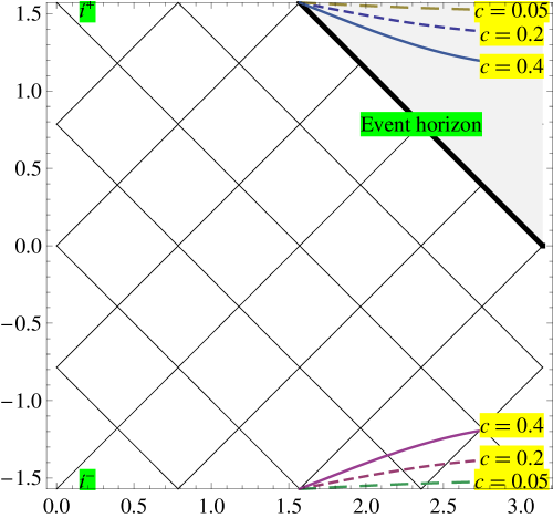
Figure 1: Penrose-Carter diagram for $\psi$-directed null geodesics. Initial and final singularities are plotted for $c=0.05$ (long dash), $c=0.2$ (short dash), $c=0.4$ (continuous). The black hole event horizon is the $z=\pi-\psi$ curve, and the gray region $z+\psi>\pi$ is the black hole region for all solutions with $c<1$.

In the terms of the conformal time $z$, the scalar field takes the following form:

$$\Phi=-\frac{1}{\zeta}\frac{\left(c\ \ \cos\psi-\cos z\right)}{\left(c\ \ \cos\psi+\cos z\right)}$$ (97)

We see from eq. 97 that the scalar field blows up at the singularity, but is regular everywhere else, including at the event horizon.

Let us look at energy conditions. The weak and strong energy conditions can be expressed in terms of the energy density $\rho$ and the principal pressures $p_{i}$ evaluated in the rest frame of the spacetime fluid Wald:1984-general . The weak energy condition requires $\rho\geq 0$ and $\rho+p_{i}\geq 0$, while the strong energy condition requires $\rho+p_{i}\geq 0$ and $\rho+\Sigma_{i}p_{i}\geq 0$. Using the Einstein equations, we may evaluate $\rho$ and $p_{i}$ from the Einstein tensor:

$$\begin{array}[]{cc}\rho=-\kappa^{-1}G_{0}^{0}&\\ p_{i}=\kappa^{-1}G_{i}^{i}&\left(i=1,2,3\right)\end{array}$$

For the metric of eq. 96, this gives

$$\rho=H_{0}^{2}\frac{{\cos}^{2}z\ \ \left(3+c^{2}(11-\cos 2z)+3\cos 2z+24c\ \ \cos z\cos\psi+2c^{2}\left(5-\cos 2z\right)\cos 2\psi\right)}{2{\left(\cos z+c\cos\psi\right)}^{4}}$$ (98)

$$\rho+p_{\psi}=H_{0}^{2}\frac{2c^{2}{\cos}^{2}z\ \ \ \left(1-\cos 2z\cos 2\psi\right)}{{\left(\cos z+c\cos\psi\right)}^{4}}$$ (99)

$$\rho+p_{\theta}=\rho+p_{\varphi}=H_{0}^{2}\frac{c^{2}{\cos}^{2}\psi{\sin}^{2}2z}{{\left(\cos z+c\cos\psi\right)}^{4}}$$ (100)

From eq. 98 it follows immediately  that the energy density is positive definite only for small $c$ ($c<1/8$) and large c ($c>24$). Furthermore, eqs. 99 and 100 yield $\rho+p_{i}\geq 0$ on all of $\mathcal{M}$. Thus, the scalar field satisifes the weak energy condition on all of $\mathcal{M}$ for $c<1/8$ or $c>24$. Furthermore,

$$\rho+\Sigma_{i}p_{i}=-H_{0}^{2}\frac{{\cos}^{2}z\ \ \left(3\left(1+\cos 2z\right)+24c\cos z\cos\psi+c^{2}(7+\cos 2z+8\cos 2\psi+2\cos 2z\cos 2\psi)\right)}{{\left(\cos z+c\cos\psi\right)}^{4}}$$

$\rho+\Sigma_{i}p_{i}$ may take both positive and negative values on $\mathcal{M}$, so the strong energy condition is generally violated on $\mathcal{M}$.

Finally, let us have a look at the equation of state parameter $w_{i}\equiv p_{i}/\rho$. Defining $u\equiv{H_{0}^{2}(\cos z+c\cos\psi)}^{-4}$, eqs. 99 and 100  allow us to write

$$w_{\psi}=-1+2c^{2}{\cos}^{2}z\ \ \ \left(1-\cos 2z\cos 2\psi\right)\frac{u}{\rho}$$ (101)

$$w_{\theta}=w_{\varphi}=-1+c^{2}({\cos}^{2}\psi{\sin}^{2}2z)\frac{u}{\rho}$$ (102)

$w_{i}>-1$ when $\rho>0$. Thus, the weak energy condition is satisfied when $\rho>0$. We also see that $w_{i}\rightarrow-1$ as $c\rightarrow 0$. This happens when the cosmological constant is much weaker than the strength of the scalar potential. In that case, we saw from eq. 97 that the scalar field is nearly constant and approaches the Planckian value $\zeta^{-1}$.

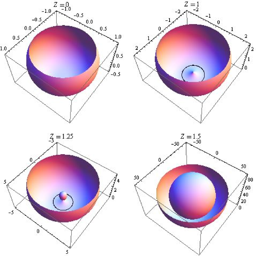
Figure 2: Time evolution of spatial geometry for $c=1/2$ (the spatial region $\psi<\pi/4$ has been chopped off). Each plot shows a fixed-time projection of the spatial geometry for  $\theta=\pi/2$. Top left: $z=0$. Top right: $z=1$. Bottom left: $z=1.25$. Bottom right: $z=1.5$. The black hole event horizon is shown as a black curve. The top two plots show the spatial geometry before the singularity has formed. The bottom two plots show the spatial geometry after the singularity has formed.  

Figure 2 shows four different snapshots of the $\theta=\pi/2$ projections of the spatial geometry of the solution. In the second plot, the spatial geometry is still regular, but it has an event horizon, shown in black. In the next plot, the singularity has formed, and a black hole has been created. The protuberance in the middle of the two plots at the bottom is a spatial region that lies beyond the singularity, and is shown in the Penrose-Carter diagram of Figure 1  as the spatial region to the right of the singularity.

Figure 3: Scalar field $\Phi$ as a function of conformal time z for the two angular positions $\psi$=0 and $\psi$=$\pi$/3. The curves are for $c=1$(continuous), $c=0.1$ (short dash) and $c=10$(long dash).

Figure 4: Equation of state parameter $w_{\psi}$ as a function of conformal time $z$ for the two angular positions $\psi$=0 and $\psi$=$\pi$/3. The curves are for $c=1$(continuous), $c=0.1$ (short dash) and $c=10$(long dash).

Figure 3 plots the scalar field as a function of conformal time $z$ and angular coordinate $\psi$ for three different values of the coordinate $c$. Figure 4 plots the equation of state parameter $w$ as a function of conformal time $z$ and angular coordinate $\psi$ for three different values of the constant $c$.

VIII Conclusions

In this paper, we generalized two previously known solution generation techniques for generating minimally coupled Einstein-scalar field solutions in 4 dimensions (the Buchdahl Buchdahl:1959nk and Fonarev Fonarev:1994xq transformations). Two generalizations were made: i) the transformation was generalized to arbitrary dimension, and ii) the new transformation allows vacuum solutions with non-zero cosmological constant as seed. Thus, we are now able to generate minimally coupled Einstein-scalar field solutions from vacuum solutions with arbitrary cosmological constant in arbitrary dimension. The only requirement to a seed solution is that it posesses a hypersurface-orthogonal  Killing vector field.

We introduced a labeling scheme that labels all solutions in terms of whether the target solution is invariant with respect to translations along the Killing vector field (class $\mathcal{S}$  solutions) or not (class $\mathcal{T}$ solutions). Furthermore, we labeled the target solution with dimension $N$, as well as whether the seed solution has non-zero cosmological constant $(\mathcal{S}_{N}^{\Lambda},\mathcal{T}_{N}^{\Lambda})$ or not ($\mathcal{S}_{N}^{0},\mathcal{T}_{N}^{0}$).

The solutions cover new, unknown solutions $(\mathcal{T}_{N}^{\Lambda})$ as well as previously known solutions, such as the solutions of Buchdahl $(S_{4}^{0})$, Fonarev ($\mathcal{T}_{4}^{0}$), Feinstein-Kunze-Vázquez-Mozo ($\mathcal{T}_{5}^{0}$) and Xanthopoulos & Zannias Xanthopoulos:1989kb (static, spherically symmetric $S_{N}^{0}$).

The generalization of the Buchdahl transformation to arbtirary dimension is new $(S_{N}^{0})$. Using the generalized Buchdahl transformation, we are able to recapture the extra-dimensional static and spherically symmetric solutions of Xanthopoulos and Zannias as a special case.

The generalization that allows us to use seed solutions with non-zero cosmological constant uncovers a new class of Einstein-scalar field solutions that has previously not been studied. We apply our solution generation technique in order to study one of the familiy of solutions, generating Einstein-scalar field solutions from the $(A){\mathrm{dS}}_{4}$ vacuum solutions. The resulting Einstein-scalar field solution that comes from transforming the de Sitter vacuum is a two-parameter family of 4 dimensional, inhomogenous, expanding cosmological solutions with $R\times S^{3}$ topology and exponential scalar potential parametrized by two parameters: the strength of the scalar potential, $W_{0}$, and the (positive) cosmological constant $\Lambda$ of the seed solution. By transforming a solution of this kind to the conformal frame using the generalized Bekenstein transformation, we find a spatially finite, expanding and accelerating cosmological solution that is conformally isometric to the Einstein universe $R\times S^{3}$. The solution can be parametrized by a cosmologial time scale $H_{0}$, defined by the strength of the scalar potential, and the inhomogeneity parameter $c$, defined by the ratio $\Lambda/W_{0}$. $H_{0}$ defines the scale of the solution, while $c$ defines the degree of spatial inhomogeneity. Low $c$ implies that the solution is highly homogeneous. We study null geodesics and find that for any observer, the solution has a cosmological event horizon at an angular distance of $\pi/2$ away from the observer. The solution has an initial singularity, which is a point singularity that vanishes at early times. The solution is then free of singularities until a final singularity emerges at late times as a new point singularity. There are timelike and null geodesics that do not intersect any of the singularities. For $c<1$, the late time singularity is hidden inside an event horizon. This family of solutions therefore has the natural interpretation of being expanding cosmologies in which a scalar black hole is formed at late times. The energy density is positive definite for small $c$ ($c<1/8\text{}$) and large $c$ ($c>24$). The conformally coupled scalar field satisfies the weak energy condition as long as the energy density is positive, while the strong energy condition is generally violated.

Appendix A Conformal transformations in arbitrary dimension

Here, we will briefly summarize how certain covariant quantities transform under conformal transformations. For a reference, see e.g. Wald:1984-general . Let $\overline{g}$ and g be the metrics of two $M$-dimensional space-time geometries that are related by a conformal transformation $\Omega^{2}$ as follows:

$${\overline{g}}_{\mu\nu}=\Omega^{2}g_{\mu\nu}$$

Let $f_{\alpha}$ be an arbitrary covariant $M$-vector. Covariant derivatives transform as follows under a conformal transformation $\Omega^{2}=e^{2\omega}$:

$$\overline{\nabla_{\alpha}}f_{\beta}=\nabla_{\alpha}f_{\beta}-\left(f_{\beta}\nabla_{\alpha}\omega+f_{\alpha}\nabla_{\beta}\omega-g_{\alpha\beta}f_{\lambda}\nabla^{\lambda}\omega\right),$$ (103)

where $\overline{\nabla_{\alpha}}$ is the covariant derivative of the metric $\overline{g}$. Recognizing that $\overline{\nabla_{\alpha}}U=$ $\partial_{\alpha}U=\nabla_{\alpha}U$, we may use equation 103 to compute how second-order covariant derivatives transform under conformal transformations:

$$\overline{\nabla_{\alpha}}\overline{\nabla_{\beta}}U=\nabla_{\alpha}\nabla_{\beta}U-\left(\nabla_{\beta}U\nabla_{\alpha}\omega+\nabla_{\alpha}U\nabla_{\beta}\omega-g_{\alpha\beta}\nabla_{\lambda}U\nabla^{\lambda}\omega\right)$$ (104)

$$\overline{\Box}U={\overline{g}}^{\alpha\beta}\overline{\nabla_{\alpha}}\overline{\nabla_{\beta}}U=e^{-2\omega}(\Box U+\left(M-2\right)\nabla^{\alpha}U\nabla_{\alpha}\omega)$$ (105)

The Ricci tensor $R_{\mu\nu}$transforms as follows under a conformal transformation $\Omega$:

$${}{}{\overline{{}R}}_{\mu\nu}\equiv R_{\mu\nu}[\overline{g}]={}{}R_{\mu\nu}[g]+\frac{2\left(M-2\right)}{\Omega^{2}}\nabla_{\mu}\Omega\nabla_{\nu}\Omega-\frac{\left(M-3\right)}{\Omega^{2}}g_{\mu\nu}\nabla^{\alpha}\Omega\nabla_{\alpha}\Omega-\frac{\left(M-2\right)}{\Omega}\nabla_{\mu}\nabla_{\nu}\Omega-\frac{1}{\Omega}g_{\mu\nu}\Box\Omega$$ (106)

Writing equation 106 in terms of $\omega$ gives:

$${}{}{\overline{{}R}}_{\mu\nu}\equiv R_{\mu\nu}[\overline{g}]={}{}R_{\mu\nu}[g]-\left(M-2\right)\nabla_{\mu}\nabla_{\nu}\omega+\left(M-2\right)\nabla_{\mu}\omega\nabla_{\nu}\omega-g_{\mu\nu}(\Box\omega+\left(M-2\right)\nabla^{\alpha}\omega\nabla_{\alpha}\omega)$$ (107)

From equation 106 we can compute the Ricci scalar of the transformed metric:

$$\overline{R}\equiv R[\overline{g}]\equiv{\overline{g}}^{\mu\nu}{\overline{R}}_{\mu\nu}=\Omega^{-2}(R[g]-\left(M-1\right)\left(\frac{2}{\Omega}\Box\Omega+\left(M-4\right)\nabla^{\alpha}\Omega\nabla_{\alpha}\Omega\right))$$ (108)

It then follows that the Einstein tensor

$${\overline{G}}_{\mu\nu}\equiv G_{\mu\nu}[\overline{g}]=R_{\mu\nu}[\overline{g}]-\frac{1}{2}{\overline{g}}_{\mu\nu}R[\overline{g}]$$

transforms as follows:

$${\overline{G}}_{\mu\nu}=G_{\mu\nu}+\frac{3\left(M-2\right)}{\Omega^{2}}\left(\Theta_{\mu\nu}[g,\Omega,\sqrt{\frac{1}{6}}]+\frac{\left(M-4\right)}{6}g_{\mu\nu}\nabla^{\alpha}\Omega\nabla_{\alpha}\Omega\right),$$ (109)

where

$$S_{\mu\nu}[g,\phi]\equiv\nabla_{\mu}\phi\nabla_{\nu}\phi-\frac{1}{2}g_{\mu\nu}\nabla^{\alpha}\phi\nabla_{\alpha}\phi$$ (110)

$$\Theta_{\mu\nu}[g,\phi,\chi]\equiv S_{\mu\nu}[g,\phi]-\chi^{2}\nabla_{\mu}\nabla_{\nu}\phi^{2}+\chi^{2}g_{\mu\nu}\Box\phi^{2}.$$ (111)

Here, g denotes an arbitrary metric,  $\phi$ denotes an arbitrary scalar function, and $\chi$ is an arbitrary constant.

Appendix B Generalized Bekenstein transformation

The non-minimally coupled Einstein-scalar field action in dimension $N$ is

$$S[g,\Phi,\xi,\Lambda,V]\equiv\int d^{N}x\sqrt{-g}\left(\frac{1}{2\kappa}\left(R-2\Lambda\right)-\frac{1}{2}\nabla^{\alpha}\Phi\nabla_{\alpha}\Phi-\frac{1}{2}\xi^{2}R\Phi^{2}-V[\Phi]\right),$$ (112)

where $\xi$ is the dimensionless scalar-gravity coupling constant. We have conformal coupling when $\xi^{2}\equiv\frac{(N-2)}{4(N-1)}$. Define $\zeta^{2}\equiv\kappa\xi$. When extremalizing this action, we obtain the conformally coupled Einstein-scalar field equations:

$$G_{\mu\nu}[g]=\frac{\kappa}{\left(1-\zeta^{2}\Phi^{2}\right)}\left(\Theta_{\mu\nu}[g,\Phi,\xi]-g_{\mu\nu}W[\Phi]\right)$$ (113)

$$\Box\Phi-\xi^{2}R\Phi-\frac{dW[\Phi]}{d\Phi}=0,$$ (114)

where $R$ is the Ricci scalar of the solution geometry and we have introduced the effective scalar potential $W[\Phi]\equiv V[\Phi]+\kappa^{-1}\Lambda$.

Let $(\overline{g},\phi,\overline{W})$ be an $N$ dimensional solution to the minimally coupled Einstein-scalar field equations, and let $(g,\Phi,W)$ be an $N$ dimensional solution to the non-minimally coupled Einstein-scalar field equations with arbitrary scalar-gravity coupling $\xi$. A Bekenstein transformation $(\Omega,f)$ is defined as a conformal transformation $\Omega^{2}$ mapping the metric $g$ into $\overline{g}$  and a function $f$ mapping the scalar field $\Phi$ into $\phi$:

$${\overline{g}}_{\mu\nu}=\Omega^{2}g_{\mu\nu}$$

$$\phi=f[\Phi]$$

Now, let us state, without proof, the generalized Bekenstein theorem in $N$ dimensions:

Theorem 9.

For every minimally coupled Einstein-scalar field solution, there are two, and only two, Bekenstein transformations that relate the minimally coupled solution to two Einstein-conformal scalar field solutions. If $(\overline{g},\phi,\overline{W})$is an $N$dimensional solution to the Einstein-scalar field equations with a minimally coupled scalar field $\phi$and a scalar field potential $\overline{W}$, there are two independent solutions $(g,\Phi,W)$, labeled A and B, to the Einstein-conformal scalar field equations, eqs. 113and 114,  given by

$$g_{\mu\nu}=\Omega^{-2}{\overline{g}}_{\mu\nu}$$ (115)

$$\Phi=\begin{cases}\frac{1}{\zeta}\tanh\zeta\phi&\left(A\right)\\ \frac{1}{\zeta}\coth\zeta\phi&\left(B\right)\\ \end{cases},$$ (116)

$$\Omega=|1-\zeta^{2}\Phi^{2}|^{\frac{1}{N-2}}=\begin{cases}{\left(\cosh\zeta\phi\right)}^{-\frac{2}{N-2}}&\left(A\right)\\ {\left(\sinh\zeta\phi\right)}^{-\frac{2}{N-2}}&\left(B\right)\\ \end{cases}$$ (117)

$$W[\Phi]=\begin{cases}\Omega^{N}\overline{W}[\phi[\Phi]]=|1-\zeta^{2}\Phi^{2}|^{\frac{N}{N-2}}\overline{W}[\phi[\Phi]]&\left(A\right)\\ -\Omega^{N}\overline{W}[\phi[\Phi]]=-|1-\zeta^{2}\Phi^{2}|^{\frac{N}{N-2}}\overline{W}[\phi[\Phi]]&\left(B\right)\\ \end{cases}$$ (118)

References

- (1) D. N. Spergel and . et. al (2006). Wilkinson Microwave Anisotropy Probe (WMAP) three year results: Implications for cosmology. arxiv:astro-ph/0603449
- (2) B. Ratra and P. J. Peebles, Phys. Rev., D37, 3406, (1988).
- (3) R. R. Caldwell, R. Dave and P. J. Steinhardt, Phys. Rev. Lett., 80, 1582, (1998).
- (4) L. Wang, R. R. Caldwell, J. P. Ostriker and P. J. Steinhardt, Astrophys. J., 530, 17, (2000).
- (5) P. G. Ferreira and M. Joyce, Phys. Rev., D58, 023503, (1998).
- (6) J. Polchinski, String Theory Volume II. Superstring Theory and Beyond (Cambridge Univ. Press, Cambridge, 1998).
- (7) O. Bertolami, J. Paramos and S. G. Turyshev (2006). General Theory of Relativity: Will it survive the next decade?. Preprint arxiv:gr-qc/0602016
- (8) I. K. Wehus and F. Ravndal (2006). Gravity coupled to a scalar field in extra dimensions. Preprint arxiv:gr-qc/0610048
- (9) H. A. Buchdahl, Phys. Rev., 115, 1325, (1959).
- (10) O. Bergmann and R. Leipnik, Phys. Rev., 107, 1157, (1957).
- (11) A. I. Janis, E. T. Newman and J. Winicour, Phys. Rev. Lett., 20, 878, (1968).
- (12) A. I. Janis, D. C. Robinson and J. Winicour, Phys. Rev., 186, 1729, (1969).
- (13) B. C. Xanthopoulos and T. Zannias, Phys. Rev., D40, 2564, (1989).
- (14) C. Callan, S. Coleman and R. Jackiw, Ann. Phys., 59, 42, (1970).
- (15) J. D. Bekenstein, Ann. Physics, 82, 535, (1974).
- (16) J. Froyland, Phys. Rev., D25, 1470, (1982).
- (17) K. Maeda, Phys. Rev., D39, 3159, (1989).
- (18) V. Husain, E. A. Martinez and D. Nunez, Phys. Rev., D50, 3783, (1994).
- (19) O. A. Fonarev, Class. Quant. Grav., 12, 1739, (1995).
- (20) A. Feinstein, K. E. Kunze and M. A. Vazquez-Mozo, Phys. Rev., D64, 084015, (2001). arxiv:hep-th/0105182
- (21) R. M. Wald, General Relativity (The University of Chicago Press, Chicago and London, 1984).