DESY 07-076
Monte Carlo Methods in Quantum Field Theory 

Abstract

In these lecture notes some applications of Monte Carlo integration methods in Quantum Field Theory – in particular in Quantum Chromodynamics – are introduced and discussed.

1 Introduction

The mathematical description of the Standard Model – the theory of elementary particle interactions – is based on relativistic Quantum Field Theory (QFT). Relativistic QFT is the quantum mechanics of fields defined on the four-dimensional space-time continuum. As such it has an infinite number of degrees of freedom – the values of field variables in every space-time point. In order to define it, one has to start with the quantum theory of a finite number of degrees of freedom: the values of field variables in a finite set of discrete points within a finite volume. In most cases the points are lattice sites of a regular, hypercubical lattice over a four-dimensional torus. In order to define the theory one has to perform the continuum limit and infinite volume limit when the spacing of the lattice points goes to zero and the extensions of the torus grow to infinity.

An important simplification from the mathematical point of view is to consider, instead of the real time variable, the time to be pure imaginary. In this Euclidean space-time the symmetry with respect to Lorentz-transformations becomes equivalent to the compact symmetry of four-dimensional rotations and, perhaps even more importantly, the quantum mechanical Schrödinger equation is transformed into an equation equivalent to the equation describing heat conduction (or e.g. the Brownian motion). The consequence is that QFT with imaginary time is equivalent to the (classical) statistical physics of the fields. In the Feynman path integral formulation of quantum mechanics the exponent in the Boltzmann-factor is the Euclidean lattice action. (Note that the “path” in case of the fields is better named as the “history” of the fields in the space-time points.)

The definition of QFT on a Euclidean space-time lattice provides a non-perturbative regularization without the infinities which have to be dealt with in perturbation theory by the renormalization procedure. One can also define perturbation theory on the lattice and in this way the lattice gives an alternative regularization for perturbation theory: the momentum cutoff is implemented by the absence of arbitrarily high momentum modes on the lattice.

The number of discrete points to be considered tends to infinity both in the continuum limit and infinite volume limit. In order to differentiate between these two infinite limits one has to consider the ratio of the effective size of physical excitations to the lattice spacing. Obviously, this ratio has to diverge in the continuum limit. In the infinite volume limit, on the other hand, the ratio of the size of physical excitations to the volume extensions is relevant. In any case, one has to know about the size of the physical excitations which is determined by the (bare) parameters in the lattice action. In the language of statistical physics, in the continuum limit one has to tune the parameters of the lattice action to some fixed point with infinite correlation lengths. If such a fixed point exists, our knowledge in statistical physics suggests universality, which means that one can reach the same fixed point (i.e. the same continuum limit) with many different lattice actions.

The most prominent example of relativistic QFT is Quantum Chromodynamics (QCD) which is the theory of strong interactions among the six known “flavors” of quarks: $u$-, $d$-, $s$-, $c$- $b$- and $t$-quark. QCD is a mathematically closed theory which has an unprecedented predictivity: it has only six independent parameters, the quark masses. More precisely the parameters of QCD are: $m_{u}/\Lambda_{QCD}$, $m_{d}/\Lambda_{QCD}$, $m_{s}/\Lambda_{QCD}$, $m_{c}/\Lambda_{QCD}$, $m_{b}/\Lambda_{QCD}$ and $m_{t}/\Lambda_{QCD}$ where the $\Lambda$-parameter of QCD $\Lambda_{QCD}$ is an arbitrary scale parameter of dimension mass. In many applications of QCD only the three “light” quarks, the $u$-, $d$- and $s$-quarks are relevant, therefore there are only three (small) parameters: $m_{u,d,s}/\Lambda_{QCD}$. All the properties of strong interactions as masses, decay widths, scattering cross-sections etc. are, in principle, determined by these parameters.

The somewhat unfortunate circumstance is that, even if in principle determined by a very small number of free parameters, it is difficult to tell what are precisely the predictions of QCD. The reason is that strong interactions are obviously (at least sometimes) strong and therefore calculational methods based on symmetries and on perturbation theory only have a limited range of applicability. The only known method to evaluate the non-perturbative predictions of QCD theory is lattice QCD. One can formulate this in a different way by saying that the validation of QCD as a true theory of strong interactions is the task of lattice QCD theorists.

In this series of (five) lectures on Monte Carlo methods first the different lattice formulations of QCD are reviewed (Section 2). The basic Monte Carlo integration methods are introduced in Section 3 and discussed in some detail, including the important methods applicable for quark dynamics (“un-quenching”). Section 4 contains a selection of some recent developments in order to illustrate recent trends in lattice QCD. Finally, the last Section 5 gives a short outlook.

2 Lattice actions

The QFT’s on the lattice are defined by their Euclidean lattice action. The lattice is in most cases a regular, hypercubical one with periodic boundary conditions (torus). Lattice elements are the sites (points) and the links connecting neighboring sites. A simple case is illustrated by the two-dimensional $4\times 4$ lattice in Figure 1. The lattice spacing is usually denoted by $a$. For the definition of lattice gauge theories like QCD the plaquettes consisting of a closed path of four links are important (see Figure 2).

The elementary excitations in QCD are the gluons and quarks. The gluons are described by a gauge field with elements in the $SU(3)$ color group $U_{x\mu}\in SU(3)_{color}$ associated with the links $(x\to x+\hat{\mu})$ where $\hat{\mu}$ denotes the unit vector in the direction $\mu\;(=1,2,3,4)$. These are parallel transporters of the color quantum number. The corresponding $SU(3)$ Lie algebra element $A_{x\mu}$ can be defined by the relation $U_{x\mu}=\exp(-aA_{x\mu})$ with the lattice spacing $a$, in order to display the mass dimension of $A_{x\mu}$. The components of $A_{x\mu}$ are introduced by $A_{x\mu}=-igA^{b}_{\mu}(x)\frac{1}{2}\lambda_{b}$, with the Gell-Mann matrices $\lambda_{b},(b=1,\ldots,8)$ and $g$ denoting the bare gauge coupling. The quark fields $\Psi$ and $\overline{\Psi}$ are associated with the lattice sites, as shown in Figure 2. (For notation conventions see, in general, the book [1].)

Figure 1: A two-dimensional periodic $4\times 4$ lattice.

Figure 2: The plaquette.

2.1 Lattice actions for gluons and quarks

2.1.1 The plaquette lattice action of the gauge field

As stated in the introduction, the lattice action for a given theory is not unique. There are large varieties of lattice actions in the same universality class realizing in the continuum limit the same QFT. For the lattice action of the $SU(3)$ color gauge field in QCD the simplest choice is the Wilson plaquette action introduced by Ken Wilson in his seminal paper on confinement and lattice QCD [2]. It is based on the definition of the field strength $F_{\mu\nu}(x)$ associated with the plaquette variable

$$U_{x;\mu\nu}\equiv U_{x,\nu}^{\dagger}U_{x+\hat{\nu},\mu}^{\dagger}U_{x+\hat{\mu},\nu}U_{x,\mu}=\exp[-a^{2}G_{\mu\nu}(x)]\ ,$$ (1)

where

$$G_{\mu\nu}(x)=F_{\mu\nu}(x)+{\cal O}(a)$$ (2)

and

$$F_{\mu\nu}(x)=\Delta^{f}_{\mu}A_{\nu}(x)-\Delta^{f}_{\nu}A_{\mu}(x)+[A_{\mu}(x),A_{\nu}(x)]$$ (3)

with the lattice forward derivative defined as $\Delta^{f}\varphi(x)\equiv\varphi(x+\hat{\mu})-\varphi(x)$.

As one can easily show, in general, for an $SU(N_{c})$ color gauge field we have

$${\rm Re\,Tr\,}U_{x;\mu\nu}=N_{c}+\frac{a^{4}}{2}{\rm\,Tr\,}F_{\mu\nu}(x)^{2}+{\cal O}(a^{5})$$ (4)

and therefore the Wilson (plaquette) gauge field action for the $SU(N_{c})$ gauge field can be defined as

$$S_{gauge}\equiv S_{g} = \sum_{x}\sum_{1\leq\mu<\nu\leq 4}\beta\left\{1-\frac{1}{N_{c}}{\rm\,Re\,Tr\,}(U_{x;\mu\nu})\right\}$$ (5)

$$= -\frac{\beta}{4N_{c}}\sum_{x\mu\nu}a^{4}{\rm\,Tr\,}F_{\mu\nu}(x)F_{\mu\nu}(x)+{\cal O}(a^{5})\ .$$

Here we introduced the usual lattice variable for the bare gauge coupling as

$$\beta\equiv\frac{2N_{c}}{g^{2}}\ .$$ (6)

An important property of the Wilson action in (5) is gauge invariance. This is due to the fact that the trace of the product of link variables along any closed path is gauge invariant because the gauge transformation of the gauge link variables is

$$U^{\prime}_{x\mu}=\Lambda^{-1}(x+\hat{\mu})\;U_{x\mu}\;\Lambda(x)\hskip 20.00003pt[\Lambda(x)\in SU(N_{c})]\ .$$ (7)

The expectation value of some function of link variables ${\cal O}[U]$ is given in terms of the invariant group (Haar-) measure $dU_{x\mu}$ as

$$\langle{\cal O}\rangle=\frac{1}{Z}\int\;\prod_{x\mu}dU_{x\mu}\;\exp\{-S_{gauge}[U]\}\;{\cal O}[U]\equiv\int[dU]\;e^{-S_{gauge}[U]}\;{\cal O}[U]\ ,$$ (8)

where the partition function for the gauge field is defined as

$$Z=\int\prod_{x\mu}dU_{x\mu}\;\exp\{-S_{gauge}[U]\}\equiv\int[dU]\;e^{-S_{gauge}[U]}\ .$$ (9)

This shows that, indeed, in the Euclidean path integral formulation lattice gauge theory is equivalent to the statistical physics of gauge fields.

2.1.2 The Wilson lattice action of fermion fields

The Dirac equation for fermions can also be similarly discretized as the equations of motion for the gauge field. A simple choice is the Wilson action for fermions:

$$S_{q}^{Wilson}=\sum_{x}\left\{\mu_{0}\overline{\psi}_{x}\psi_{x}-\frac{1}{2}\sum_{\mu}\overline{\psi}_{x+\hat{\mu}}\gamma_{\mu}U_{x\mu}\psi_{x}-\frac{r}{2}\sum_{\mu}[\overline{\psi}_{x+\hat{\mu}}U_{x\mu}-\overline{\psi}_{x}]\psi_{x}\right\}\ .$$ (10)

Here $\psi_{x},\;\overline{\psi}_{x}$ are anticommuting Grassmann variables which have, in general, a Dirac-spinor, a color and a flavor index. For a single species (“flavor”) of fermions, of course, there is just a spinor and a color index. The lattice spacing is set now to unity: $a\equiv 1$, which is often done in the literature. $\mu_{0}$ is the bare quark mass in lattice units and the Wilson parameter is $r\neq 0$. The summation in (10) runs over both positive and negative directions: $\sum_{\mu}\equiv\sum_{\mu=\pm 1}^{\pm 4}$ and, by definition, we have $\gamma_{-\mu}=-\gamma_{\mu}$. The role of the Wilson term proportional to $r$ will be discussed below. In (10) the interaction of the fermion with a gauge field is introduced by the gauge link variables $U_{x\mu}$. Free fermions with no interaction correspond to $U_{x\mu}=1$.

Often used notations are based on redefining the field normalizations according to

$$(\mu_{0}+4r)^{1/2}\;\psi_{x}\;\Rightarrow\;\psi_{x}\ ,\hskip 20.00003pt(\mu_{0}+4r)^{1/2}\;\overline{\psi}_{x}\;\Rightarrow\;\overline{\psi}_{x}$$ (11)

and introducing the hopping parameter by

$$\kappa\equiv(2\mu_{0}+8r)^{-1}\ ,\hskip 30.00005pt\mu_{0}=\frac{1}{2}(\kappa^{-1}-8r)\ .$$ (12)

In this way the Wilson action (10) can be rewritten as

$$S_{q}^{Wilson}=\sum_{x}\left\{(\overline{\psi}_{x}\psi_{x})-\kappa\sum_{\mu}(\overline{\psi}_{x+\hat{\mu}}U_{x\mu}[r+\gamma_{\mu}]\psi_{x})\right\}\equiv\sum_{xy}(\overline{\psi}_{y}Q_{yx}\psi_{x})\ .$$ (13)

In the second form the Wilson fermion matrix is (without explicit color- and Dirac-indices):

$$Q_{yx}=\delta_{yx}-\kappa\sum_{\mu}\delta_{y,x+\hat{\mu}}\;U_{x\mu}\;(r+\gamma_{\mu})\ .$$ (14)

The particle excitations of Wilson lattice fermions can be identified by considering the Wilson fermion propagator, which is defined by the inverse of the (free) fermion matrix in (14):

$$\sum_{y}\Delta_{zy}Q_{yx}=\delta_{zx}\ ,\hskip 30.00005pt\Delta_{yx}=\Delta_{y-x}=\frac{1}{\Omega}\sum_{k}e^{ik\cdot(y-x)}\tilde{\Delta}_{k}\ .$$ (15)

Here $\Omega=N_{1}N_{2}N_{3}N_{4}$ is the number of lattice points and the allowed values of the momenta for periodic and antiperiodic boundary conditions, respectively, are

$$ap_{\mu}\equiv k_{\mu}=\frac{2\pi}{N_{\mu}}\nu_{\mu}\ ,\hskip 20.00003ptk_{\mu}=\frac{2\pi}{N_{\mu}}\left(\nu_{\mu}+\frac{1}{2}\right)\hskip 20.00003pt(\nu_{\mu}\in\{0,1,2,\dots,N_{\mu}-1\})\ .$$ (16)

Using the notations

$$\hat{k}_{\mu}\equiv 2\sin\frac{k_{\mu}}{2}\ ,\hskip 30.00005pt\bar{k}_{\mu}\equiv\sin k_{\mu}\ ,$$ (17)

the solution of Eq. (15) is given by

$$\tilde{\Delta}_{k}=\frac{1-r\kappa(8-\hat{k}^{2})-2i\kappa\gamma\cdot\bar{k}}{[1-r\kappa(8-\hat{k}^{2})]^{2}+4\kappa^{2}\bar{k}^{2}}=(2\kappa)^{-1}\;\frac{\mu_{0}+(r/2)\hat{k}^{2}-i\gamma\cdot\bar{k}}{[\mu_{0}+(r/2)\hat{k}^{2}]^{2}+\bar{k}^{2}}\ .$$ (18)

Particle excitations belong to the poles of the propagator. Considering the Wilson fermion propagator in (18), it becomes clear why the non-zero value of the Wilson parameter $r$ is required, namely, for avoiding additional particle poles at $k_{\mu}=\pi$ besides the physical ones at $k_{\mu}=0$. For $r=0$, which corresponds to the naive discretization of the Dirac equation, these additional particles emerge and – instead of a single fermion flavor – sixteen flavors are described. The 15 extra unphysical particles are the consequence of the first order character of the Dirac equation. Introducing a non-zero $r$ removes the unphysical fermions from the spectrum in the continuum limit ($a\to 0$) because their masses tend to infinity as $a^{-1}$. The price to pay for repairing the particle content is, however, rather high because for $r\neq 0$ the chiral symmetry is broken also for zero fermion mass!

2.1.3 The Kogut-Susskind staggered lattice action of fermion fields

As discussed in the previous subsection, the “naive” fermion action without the Wilson term (i.e. $r=0$) describes 16 fermion “flavors”. The naive fermion action is:

$$S_{q}^{naive}=\sum_{x}\left\{\mu_{0}\overline{\Psi}_{x}\Psi_{x}+\frac{1}{2}\sum_{\mu=1}^{4}\left[\overline{\Psi}_{x}\gamma_{\mu}\Psi_{x+\hat{\mu}}-\overline{\Psi}_{x+\hat{\mu}}\gamma_{\mu}\Psi_{x}\right]\right\}\ .$$ (19)

One can perform on this a spin diagonalization by a transformation

$$\Psi_{x}=A_{x}\psi_{x}\ ,\hskip 40.00006pt\overline{\Psi}_{x}=\overline{\Psi}_{x}A^{\dagger}_{x}$$ (20)

in such a way that

$$A^{\dagger}_{x}\gamma_{\mu}A_{x}=\alpha_{x\mu}{\bf\;1_{4}}=(-1)^{x_{1}+\cdots+x_{\mu-1}}{\bf\;1_{4}}\ ,\hskip 20.00003pt(\mu=1,2,3,4)\ .$$ (21)

One out of four identical components gives the “staggered” fermion action:

$$S_{q}^{staggered}=\sum_{x}\left\{\mu_{0}\overline{\psi}_{x}\psi_{x}+\frac{1}{2}\sum_{\mu=1}^{4}\alpha_{x\mu}\;\left[\overline{\psi}_{x}\psi_{x+\hat{\mu}}-\overline{\psi}_{x+\hat{\mu}}\psi_{x}\right]\right\}\ .$$ (22)

The staggered fermion action describes four degenerate flavors with components scattered on the points of $2^{4}$ hypercubes. (Note that there are no Dirac spinor indices for staggered lattice fermions – only color indices!) Rather remarkably, at zero fermion mass $\mu_{0}=0$ there is a remainder of exact chiral symmetry, namely, $\;U_{even}(1)\otimes U_{odd}(1)$.

2.2 Improved fermion actions

The freedom of choosing the lattice action in the universality class of the same limiting theory in the continuum can be used for:

• accelerating the convergence to the continuum limit,

• achieving enhanced symmetries already at non-zero lattice spacings.

In QCD particularly interesting is the improvement of chiral symmetry at non-zero lattice spacings which implies, for instance, simpler renormalization patterns for composite (e.g. current-) operators.

The basic tools for constructing improved actions are lattice perturbation theory, renormalization group transformations [3] and the local effective theories at non-zero cut-off [4, 5].

Great effort has been invested recently in constructing improved actions for staggered quarks (see, for instance, the papers of the MILC Collaboration [6]). In the so called Asqtad action the gauge action includes a combination of the plaquette, the $1\times 2$ rectangle and a bent parallelogram 6-link term. The quark action includes paths up to seven links of the form $\overline{\psi}_{y}U_{y\leftarrow x}\psi_{x}$ where $U_{y\leftarrow x}$ is the product of links along the path $x\rightarrow y$. The relative weight of the contributions is such that the flavor symmetry breaking is suppressed and the small momentum behavior is improved. Since one staggered quark field describes four “flavors” of fermions (called here “tastes”), for describing a single quark flavor in the path integral the fourth root of the fermion matrix is taken (“rooting”):

$$\int[dU\,d\overline{\psi}\,d\psi]\,e^{-S_{g}-S_{q}}=\int[dU]\,e^{-S_{g}}\det Q\;\;\Rightarrow\;\;\int[dU]\,e^{-S_{g}}\,(\det Q)^{1/4}\ .$$ (23)

It is assumed (but debated) that this gives the correct continuum limit.

2.2.1 Twisted-mass lattice QCD

A particularly simple way of improving the Wilson-fermion action is the chiral rotation of the Wilson term in $S_{q}^{Wilson}$ Eq. (10) [7, 8]. For two equal mass quark flavors ($N_{f}=2$) the unbroken $SU(2)$ subgroup of the $SU(2)\otimes SU(2)$ chiral symmetry can be partly rotated to axialvector directions. In addition, “automatic” ${\cal O}(a)$ improvement is possible [9].

The twisted mass lattice fermion action is:

$$S_{q}^{tm} = \sum_{x}\left\{a\mu_{q}\overline{\psi}_{x}\psi_{x}-\frac{1}{2}\sum_{\mu}\overline{\psi}_{x+\hat{\mu}}\gamma_{\mu}U_{x\mu}\psi_{x}\right.$$ (24)

$$+ \left.a\mu_{cr}\overline{\psi}_{x}e^{-i\omega\gamma_{5}\tau_{3}}\psi_{x}-\frac{r}{2}\sum_{\mu}[\overline{\psi}_{x+\hat{\mu}}U_{x\mu}-\overline{\psi}_{x}]e^{-i\omega\gamma_{5}\tau_{3}}\psi_{x}\right\}\ .$$

Here $\omega$ is the twist angle, $a\mu_{q}$ the bare quark mass in lattice units and $a\mu_{cr}=(\frac{1}{2}\kappa_{cr}^{-1}-4r)<0$ the critical bare quark mass where $\mu_{q}^{physical}=0$.

The “twist” can be moved to the mass term by a chiral transformation

$$\chi_{x}=\exp(-\frac{i}{2}\omega\gamma_{5}\tau_{3})\psi_{x}\ ,\hskip 20.00003pt\overline{\chi}_{x}=\overline{\psi}_{x}\exp(-\frac{i}{2}\omega\gamma_{5}\tau_{3})\ ,$$ (25)

hence the name “twisted mass”. Introducing the quark mass variables

$$\mu_{\kappa}\equiv a\mu_{cr}+a\mu_{q}\cos\omega\equiv\frac{1}{2\kappa}=am_{0}+4r\ ,\hskip 20.00003pta\mu\equiv a\mu_{q}\sin\omega\ ,$$ (26)

the action in (25) becomes

$$S_{q}^{tm} = \sum_{x}\left\{\left(\overline{\chi}_{x}[\mu_{\kappa}+i\gamma_{5}\tau_{3}\,a\mu]\chi_{x}\right)-\frac{1}{2}\sum_{\mu=\pm 1}^{\pm 4}\left(\overline{\chi}_{x+\hat{\mu}}U_{x\mu}[r+\gamma_{\mu}]\chi_{x}\right)\right\}$$ (27)

$$\equiv \sum_{x,y}\overline{\chi}_{x}Q^{(\chi)}_{xy}\chi_{y}\ .$$

In numerical simulations one starts with this form because it does not contain the critical quark mass $a\mu_{cr}$ which is à priori unknown and has to be first numerically determined. Near maximal twist corresponding to $\omega=\pi/2$ it is also convenient to introduce till another fermion field by the transformations:

$$\Psi_{x}\equiv\frac{1}{\sqrt{2}}\left(1+i\gamma_{5}\tau_{3}\right)\chi_{x}\ ,\hskip 30.00005pt\overline{\Psi}_{x}\equiv\overline{\chi}_{x}\frac{1}{\sqrt{2}}\left(1+i\gamma_{5}\tau_{3}\right)\ .$$ (28)

The quark matrix on the $\chi$-basis $Q^{(\chi)}$ defined in (27) is

$$Q^{(\chi)}_{xy}=\delta_{xy}\left(\mu_{\kappa}+i\gamma_{5}\tau_{3}\,a\mu\right)-\frac{1}{2}\sum_{\mu=\pm 1}^{\pm 4}\delta_{x,y+\hat{\mu}}U_{y\mu}[r+\gamma_{\mu}]$$ (29)

or in a short notation, without the site indices,

$$Q^{(\chi)}=\mu_{\kappa}+i\gamma_{5}\tau_{3}\,a\mu+N+R\ ,$$ (30)

with

$$N_{xy}\equiv-\frac{1}{2}\sum_{\mu=\pm 1}^{\pm 4}\delta_{x,y+\hat{\mu}}U_{y\mu}\gamma_{\mu}\ ,\hskip 20.00003ptR_{xy}\equiv-\frac{r}{2}\sum_{\mu=\pm 1}^{\pm 4}\delta_{x,y+\hat{\mu}}U_{y\mu}\ .$$ (31)

On the $\Psi$-basis defined in (28) we have the quark matrix

$$Q^{(\Psi)}=\frac{1}{2}\left(1-i\gamma_{5}\tau_{3}\right)Q^{(\chi)}\left(1-i\gamma_{5}\tau_{3}\right)=a\mu+N-i\gamma_{5}\tau_{3}\left(\mu_{\kappa}+R\right)\ .$$ (32)

The quark determinant in the path integral over the gauge field is, for instance, using the quark mass variables in (24):

$$\det\left[(D^{cr}+a\mu_{q}\cos\omega)^{\dagger}(D^{cr}+a\mu_{q}\cos\omega)+(a\mu_{q})^{2}\sin^{2}\omega\right]$$ (33)

where the single-flavor critical fermion matrix is

$$D^{cr}_{yx}=a\mu_{cr}\delta_{yx}-\frac{1}{2}\sum_{\mu}\left[\delta_{y,x+\hat{\mu}}\gamma_{\mu}U_{x\mu}+r(\delta_{y,x+\hat{\mu}}U_{x\mu}-\delta_{yx})\right]$$ (34)

An important feature of the twisted mass formulation is that the fermion matrix

$$D^{cr}+a\mu_{q}(\cos\omega+i\gamma_{5}\tau_{3}\sin\omega)$$ (35)

cannot have zero eigenvalues for non-zero quark mass if $\omega\neq 0,\pi$. There are no spurious zero modes and hence no exceptional gauge configurations with anomalously small eigenvalues of the fermion matrix. This makes the Monte Carlo simulations at small quark- (and pion-) mass easier.

The consequence of the chiral rotation corresponding to the twist is that the directions of vector- and axialvector-symmetries in the $SU(2)\otimes SU(2)$ chiral group are also rotated. One can achieve conserved axialvector currents but then some of the vector- (flavor-) symmetries will be broken. (The twist also induces a breaking of parity.) The status and consequences of the chiral symmetry can be deduced from the chiral $SU(2)\otimes SU(2)$ Ward-Takahashi-identities.

Exactly conserved axialvector currents can be achieved at $\omega=\frac{1}{2}\pi$. In this special case the conserved currents are: two axialvector currents ($j=1,2$ )

$$A^{con}_{jx\mu} = \frac{1}{2}\left\{\left(\overline{\psi}_{x+\hat{\mu}}\gamma_{\mu}\gamma_{5}\frac{\tau_{j}}{2}U_{x\mu}\psi_{x}\right)+\left(\overline{\psi}_{x}\gamma_{\mu}\gamma_{5}\frac{\tau_{j}}{2}U_{x\mu}^{\dagger}\psi_{x+\hat{\mu}}\right)\right.$$ (36)

$$+ \left.r\left(\overline{\psi}_{x+\hat{\mu}}\frac{\overline{\tau}_{j}}{2}U_{x\mu}\psi_{x}\right)-r\left(\overline{\psi}_{x}\frac{\overline{\tau}_{j}}{2}U_{x\mu}^{\dagger}\psi_{x+\hat{\mu}}\right)\right\}$$

with $\overline{\tau}_{1}\equiv\tau_{2}$ and $\overline{\tau}_{2}\equiv-\tau_{1}$, and one vector current:

$$V^{con}_{3x\mu} = \frac{1}{2}\left\{\left(\overline{\psi}_{x+\hat{\mu}}\gamma_{\mu}\frac{\tau_{3}}{2}U_{x\mu}\psi_{x}\right)+\left(\overline{\psi}_{x}\gamma_{\mu}\frac{\tau_{3}}{2}U_{x\mu}^{\dagger}\psi_{x+\hat{\mu}}\right)\right.$$ (37)

$$- \left.\frac{ir}{2}\left(\overline{\psi}_{x+\hat{\mu}}\gamma_{5}U_{x\mu}\psi_{x}\right)+\frac{ir}{2}\left(\overline{\psi}_{x}\gamma_{5}U_{x\mu}^{\dagger}\psi_{x+\hat{\mu}}\right)\right\}\ .$$

The invariance of the path integral with respect to the change of variables

$$\psi^{\prime}_{x} = (1+\frac{i}{2}\alpha_{Vrx}\tau_{r}+\frac{i}{2}\alpha_{Arx}\gamma_{5}\tau_{r})\psi_{x}\ ,$$

$$\overline{\psi}^{\prime}_{x} = \overline{\psi}_{x}(1-\frac{i}{2}\alpha_{Vrx}\tau_{r}+\frac{i}{2}\alpha_{Arx}\gamma_{5}\tau_{r})$$ (38)

implies for an arbitrary function ${\cal O}$ of field variables the following WT-identities:

$$\left\langle{\cal O}\;\Delta^{b}_{\mu}A^{con}_{jx\mu}\right\rangle+\left\langle\frac{{\cal O}\stackrel{{\scriptstyle\leftarrow}}{{\partial}}}{\partial\psi_{x}}\;\gamma_{5}\frac{\tau_{j}}{2}\psi_{x}+\overline{\psi}_{x}\gamma_{5}\frac{\tau_{j}}{2}\;\frac{\stackrel{{\scriptstyle\rightarrow}}{{\partial}}{\cal O}}{\partial\overline{\psi}_{x}}\right\rangle = \mu_{q}\left\langle{\cal O}\;\overline{\psi}_{x}\gamma_{5}\tau_{j}\psi_{x}\right\rangle$$

$$\left\langle{\cal O}\;\Delta^{b}_{\mu}V^{con}_{3x\mu}\right\rangle+\left\langle\frac{{\cal O}\stackrel{{\scriptstyle\leftarrow}}{{\partial}}}{\partial\psi_{x}}\;\frac{\tau_{3}}{2}\psi_{x}-\overline{\psi}_{x}\frac{\tau_{3}}{2}\;\frac{\stackrel{{\scriptstyle\rightarrow}}{{\partial}}{\cal O}}{\partial\overline{\psi}_{x}}\right\rangle = 0\ ,$$ (39)

with the backward lattice derivative defined as $\Delta^{b}_{\mu}\varphi(x)\equiv\varphi(x)-\varphi(x-\hat{\mu})$.

Besides the conserved axialvector currents the important feature of twisted-mass Wilson fermions is automatic ${\cal O}(a)$ improvement. (${\cal O}(a)$ improvement means that in the continuum limit $a\to 0$ the leading deviation from the limiting value behaves asymptotically as ${\cal O}(a^{2})$.) As it has been shown by Frezzotti and Rossi [9], for the (untwisted) Wilson fermion action we have

$$\langle{\cal O}\rangle^{WA}_{(m_{q})}\equiv\frac{1}{2}\left[\langle{\cal O}\rangle_{(r,m_{q})}+\langle{\cal O}\rangle_{(-r,m_{q})}\right]\propto\langle{\cal O}\rangle^{cont}_{(m_{q})}+{\cal O}(a^{2})\ .$$ (40)

This is averaging over opposite sign Wilson parameters: “Wilson average”.

In twisted mass lattice QCD (tmLQCD) changing the sign of $r$ is equivalent to shifting the twist angle by $\pi$. In the special case of $\omega=\frac{1}{2}\pi$ this is equivalent to $\omega\rightarrow-\omega$, therefore expectation values even in $\omega$ are “automatically” ${\cal O}(a)$ improved, without any averaging. Automatically ${\cal O}(a)$ improved physical quantities are, for instance:

• the energy eigenvalues, hence the masses;

• on-shell matrix elements at zero spatial momenta;

• matrix elements of operators with parity equal to the product of the parities of the external states.

2.2.2 Domain wall lattice fermions

The chiral symmetry of massless fermions can be realized at non-zero lattice spacing by introducing a fifth “extra dimension” [10, 11, 12]. In the fifth direction there is a “defect”: either the mass term changes sign [10] or there are “walls” at the two ends [12]. In this case there are chiral fermion solutions which are exponentially localized in the fifth dimension near these defects. The gauge field remains four-dimensional (independent on the fifth dimension). In the limit of infinitely large fifth dimension the positive and negative chirality solutions (at opposite walls or at opposite sign changes on a torus) have zero overlap with each other and the chiral symmetry becomes exact.

The domain wall fermion action can be written (with $1\leq s\leq N_{s}$) as

$$S_{F}=\sum_{s,s^{\prime}}\overline{\Psi}_{xs}(D_{F})_{xs,x^{\prime}s^{\prime}}\Psi_{x^{\prime}s^{\prime}}$$ (41)

where in an $s$-block form

$$D_{F}=\left(\begin{array}[]{cccccccc}\sigma+D&-\sigma P_{L}&0&0&\ldots&0&0&m_{f}P_{R}\\[6.99997pt] -\sigma P_{R}&\sigma+D&-\sigma P_{L}&0&\ldots&0&0&0\\[6.99997pt] 0&-\sigma P_{R}&\sigma+D&-\sigma P_{L}&\ldots&0&0&0\\[6.99997pt] \vdots&\vdots&\vdots&\vdots&\ddots&\vdots&\vdots&\vdots\\[6.99997pt] 0&0&0&0&\ldots&-\sigma P_{R}&\sigma+D&-\sigma P_{L}\\[6.99997pt] m_{f}P_{L}&0&0&0&\ldots&0&-\sigma P_{R}&\sigma+D\end{array}\right)\ .$$ (42)

The chiral projectors are denoted, as usual, by $P_{R,L}\equiv\frac{1}{2}(1\pm\gamma_{5})$, the quark mass in lattice units is $m_{f}$, the ratio of lattice spacings is $\sigma=a/a_{s}$ and the four-dimensional Wilson-Dirac matrix with negative mass ($0>-m_{0}>-2$) is, for $r=1$,

$$D_{xx^{\prime}}=(4-m_{0})\delta_{xx^{\prime}}\;-\;\frac{1}{2}\sum_{\mu=1}^{4}\left[\delta_{x^{\prime},x+\hat{\mu}}(1+\gamma_{\mu})U_{x\mu}+\delta_{x^{\prime}+\hat{\mu},x}(1-\gamma_{\mu})U^{\dagger}_{x^{\prime}\mu}\right]\ .$$ (43)

The hermitian fermion matrix corresponding to $D_{F}$ in (42) is useful, for instance, in Monte Carlo simulations. It can be constructed as follows: since with an $s$-reflection $(R_{5})_{ss^{\prime}}\equiv\delta_{N_{s}+1-s,s^{\prime}}$ we have

$$D_{F}=R_{5}\gamma_{5}D_{F}^{\dagger}R_{5}\gamma_{5}\ ,$$ (44)

the hermitian fermion matrix can be defined as

$$\tilde{D}_{F}\equiv R_{5}\gamma_{5}D_{F}=\tilde{D}_{F}^{\dagger}\ .$$ (45)

The chiral symmetry is broken by a non-zero overlap of the opposite chirality wave functions, which tends to zero in the limit of an infinite extension of the fifth dimension: $N_{s}\to\infty$. Enhanced symmetry breaking occurs if the four-dimensional Wilson fermion matrix $D$ has small eigenvalues.

2.2.3 Neuberger overlap fermions

Another possibility to achieve chiral symmetry of the lattice fermion action, which in fact can be related to domain wall lattice fermions, is the Neuberger (overlap-) fermion action.

Let us rewrite the (free) Wilson fermion action for $r=1$ and $\mu_{0}\equiv am_{0}$ as

$$S_{q}^{Wilson} = \sum_{x}a^{4}\,\overline{\psi}_{x}[m_{0}+D_{W}]\psi_{x}\ ,$$

$$D_{W} \equiv \sum_{\mu=1}^{4}\left[\frac{1}{2}\gamma_{\mu}(\nabla_{\mu}+\nabla^{*}_{\mu})-\frac{a}{2}\,\nabla^{*}_{\mu}\nabla_{\mu}\right]\ ,$$ (46)

where the lattice derivatives are now denoted by

$$\nabla_{\mu}\equiv a^{-1}\Delta^{f}_{\mu}\ ,\hskip 30.00005pt\nabla^{*}_{\mu}\equiv a^{-1}\Delta^{b}_{\mu}\ .$$ (47)

The Neuberger lattice fermion operator with zero mass is defined as

$$D_{N}\equiv\frac{1}{a}\left(1-A\,\frac{1}{\sqrt{A^{\dagger}A}}\right)\ ,\hskip 30.00005ptA\equiv 1-aD_{W}\ .$$ (48)

The inverse square-root here can be realized by polynomial or rational approximations. Note that $A$ is proportional to the Wilson fermion matrix with bare mass $-a^{-1}$.

An important property of the Neuberger operator $D_{N}$ is that $V\equiv 1-aD_{N}$ is unitary: $V^{\dagger}V=1$. As a consequence, the spectrum of $D_{N}=a^{-1}(1-V)$ is on a circle going through the origin. In addition, the Neuberger operator satisfies the Ginsparg-Wilson relation

$$\gamma_{5}D_{N}+D_{N}\gamma_{5}=aD_{N}\gamma_{5}D_{N}\ .$$ (49)

This is equivalent to the condition as introduced by Ginsparg and Wilson (GW) [13]

$$\gamma_{5}D^{-1}+D^{-1}\gamma_{5}=2aR\gamma_{5}\ .$$ (50)

The GW-relation is the optimal approximation to chiral symmetry which can be realized by a lattice fermion operator for $a\to 0$. $R$ in (50) is, in general, a local operator. For the Neuberger operator $D=D_{N}$ we have $R=\frac{1}{2}$.

The lattice chiral symmetry satisfied by a GW-lattice fermion can be explicitely displayed by appropriately defined chiral transformations [14]. It can be shown that

$$\delta\psi=\gamma_{5}\left(1-\frac{a}{2}D\right)\psi\ ,\hskip 30.00005pt\delta\overline{\psi}=\overline{\psi}\left(1-\frac{a}{2}D\right)\gamma_{5}$$ (51)

is an exact chiral symmetry for any lattice spacing $a$ if the GW-relation is satisfied.

Lattice actions satisfying the GW-relation are:

• the fixed point action, which is the fixed point of some renormalization group transformation [15];

• the Neuberger action $D_{N}$ in (48);

• the effective (four-dimensional) action of the light fermion field of the domain wall fermion [16].

Note: the inverse of the effective Dirac operator of the light fermion field of the domain wall fermion is equivalent to the inverse of the truncated overlap Dirac operator (except for a local contact term). Using GW-fermions one can prove the index theorem about topological charge [17] and introduce the $\theta$-parameter in QCD, etc.

Having lattice actions with exact chiral symmetry at non-zero lattice spacing is a great achievement. Although it is expected that (spontaneously broken) chiral symmetry is restored in the continuum limit also for simple lattice formulations with, for instance, Wilson fermions, the explicit breaking of chiral symmetry for non-zero lattice spacings makes the renormalization of composite operators more involved and in practice also much more cumbersome because of the extended mixing pattern. The chiral symmetry restricts the mixing to be simpler and more tractable.

The difficulty of defining chiral symmetric lattice actions is emphasized by the Nielsen-Ninomiya theorem [18]. This theorem states that there is no (free) lattice fermion action which can be written in the form

$$S_{f}=a^{4}\sum_{xy}\overline{\psi}_{y}D(y-x)\psi_{x}$$ (52)

and which would simultaneously satisfy the following conditions:

• $D(x)$ is local (bounded for large $x$ by $e^{-\gamma|x|}$),

• its Fourier-transform is $\tilde{D}(p)=i\gamma_{\mu}p_{\mu}+{\cal O}(ap^{2})$ for $p\ll\pi/a$,

• $\tilde{D}(p)$ is invertible for $p\neq 0$ (i.e. there are no massless fermion doubler poles),

• $\gamma_{5}D+D\gamma_{5}=0$ (chiral symmetry).

GW-fermions circumvent the Nielsen-Ninomiya theorem by relaxing the last condition: instead of exact anticommutativity only a weaker condition, namely the Ginsparg-Wilson relation in (49), is satisfied. Correspondingly, the chiral transformation is modified: the simple continuum transformation is generalized to (51).

The important question is whether the locality of the action is ensured for GW-fermions. In case of the Neuberger (overlap) action locality can be proven if the gauge field is smooth enough, namely if every plaquette value is close to unity [19]. Because of the importance of locality such gauge fields are sometimes called “admissible”. Of course, usual lattice actions typically admit any plaquette value and therefore in the path integral “inadmissible” configurations also occur. In fact, in actual simulations there are always plaquettes with small values. It is an open question whether this turns out to be a problem in the continuum limit. In any case, the lattice spacing has to be small enough in order to avoid the “Aoki phase” with lots of small eigenvalues of $D_{W}$. The small eigenvalues make $D_{N}$ non-local and the “residual mass” breaking the chiral symmetry of domain wall fermions large [20].

3 Monte Carlo integration methods

The goal of numerical simulations in Quantum Field Theories (QFT’s) is to estimate the expectation value of some functions $A[\varphi]$ of the field variables generically denoted by $[\varphi]\equiv\{\varphi_{x\alpha}\}$. In terms of path integrals this is given as

$$\langle A\rangle=Z^{-1}\int[d\varphi]e^{-S[\varphi]}A[\varphi]\ ,\hskip 30.00005ptZ=\int[d\varphi]e^{-S[\varphi]}\ .$$ (53)

$S[\varphi]$ is the lattice action, which is assumed to be a real function of the field variables. (To begin with, we only consider bosonic path integrals.)

A typical lattice action contains a summation over the lattice sites. Since the number of lattice points $\Omega$ is large, there are many integration variables. However, since (53) corresponds to a statistical system with a large number of degrees of freedom, in the path integral only a small vicinity of the minimum of the “free energy” density will substantially contribute. A suitable mathematical method to treat with such situations is Monte Carlo integration. (For a recent review of Monte Carlo integration in QFT’s see Ref. [21].)

3.1 Monte Carlo integration

3.1.1 Simple Monte Carlo integration

Let us consider a continuous real function $f(X)$ of a continuous random variable $X$ having probability distribution $p_{X}(s)$ and hence the expectation value

$$\langle f(X)\rangle=\int ds\,f(s)\,p_{X}(s)\ .$$ (54)

Using $p_{X}(s)$ to obtain $N$ outcomes of $X$ ($X_{1},X_{2},\ldots,X_{N}$), the random variables $Y_{j}=f(X_{j})$ give

$$\lim_{N\to\infty}\frac{1}{N}\sum_{j=1}^{N}Y_{j}=\langle Y\rangle=\langle f(X)\rangle=\int ds\,f(s)\,p_{X}(s)\ .$$ (55)

In a short notation:

$$\overline{f}\equiv\frac{1}{N}\sum_{j=1}^{N}f(X_{j}),\hskip 30.00005pt\lim_{N\to\infty}\overline{f}=\langle f\rangle=\int ds\,f(s)\,p_{X}(s)\ .$$ (56)

For large $N$, the central limit theorem tells us that the error in approximating $\langle f(X)\rangle$ is given by the variance $V[f(X)]$ as $\sqrt{V[f(X)]/N}$. The Monte Carlo estimate of the variance is:

$$V[Y]=\left\langle(Y-\langle Y\rangle)^{2}\right\rangle\approx\overline{(f-\overline{f})^{2}}=\overline{f^{2}}-\overline{f}^{2}\ .$$ (57)

Generalizing this to several ($D$) integration variables one obtains the following formulas for simple Monte Carlo integration:

$$\int_{\cal V}d^{D}x\,p(\vec{x})\,f(\vec{x})\approx\overline{f}\pm\left(\frac{\overline{f^{2}}-\overline{f}^{2}}{N}\right)^{\frac{1}{2}}\ .$$ (58)

Here, according to the notation introduced in (56),

$$\overline{f}\equiv\frac{1}{N}\sum_{i=1}^{N}f(\vec{x}_{i}),\hskip 30.00005pt\overline{f^{2}}\equiv\frac{1}{N}\sum_{i=1}^{N}f(\vec{x}_{i})^{2}\ .$$ (59)

The points $\vec{x}_{1},\vec{x}_{2},\ldots,\vec{x}_{N}$ have to be chosen independently and randomly with probability distribution $p(\vec{x})$ in the $D$-dimensional volume $\cal V$.

3.1.2 Importance sampling

Simple Monte Carlo integration works best for flat functions but is problematic if the integrand is sharply peaked or rapidly oscillating. Therefore, a good procedure is to apply importance sampling: find a positive function $g(x)$ with integral norm unity ($\int dx\,g(x)=1$) such that $h(x)\equiv f(x)/g(x)$ is as close as possible to a constant and then calculate

$$\int_{a}^{b}dx\,f(x)=\int_{a}^{b}dx\,g(x)h(x)\approx\frac{(b-a)}{N}\sum_{j=1}^{N}h(x_{j})\ ,$$ (60)

where the points $x_{j}$ are chosen with probability density $g(x)$ and we used simple Monte Carlo integration with a constant probability in an interval:

$$\int_{a}^{b}dx\,f(x)\approx\frac{(b-a)}{N}\sum_{j=1}^{N}f(x_{j})\ .$$ (61)

The prerequisite is, of course, that one can find an appropriate $g(x)$ such that on can generate points with it.

How can one generate the desired (in general, multi-dimensional) probability distributions? One possibility for lower-dimensional integrals is the rejection method. This is based on the observation that sampling with $p_{X}(x)$, for instance, in an interval $x\in[b,a]$ is equivalent to choose a random point uniformly in two dimensions and reject it unless it is in the area under the curve $p_{X}(x)$. For high-dimensional distributions this becomes cumbersome. Multi-dimensional integrals can be handled by exploiting Markov processes.

3.1.3 Markov chains

A Markov process (or “Markov chain”) is a sequence of states which are generated with transition probabilities from a given state to the next one. The transition probability is assumed to depend only on the current state of the system and not on any previous state. For simplicity, for discrete states $s_{1},s_{2},\ldots,s_{R}$ the transition probability can be denoted by $p_{ij}$. The matrix $\bf P$ with elements $p_{ij}$ is called transition matrix (or Markov-matrix).

The mathematical properties of Markov chains are extensively covered in the literature. For a comprehensive collection of features relevant in Monte Carlo integration of QFT’s see Ref. [21]. Let us mention here just a few of them:

• The product of two Markov matrices $\bf P_{1}P_{2}$ is again a Markov matrix.

• Every eigenvalue of a Markov matrix satisfies $|\lambda|\leq 1$.

• Every Markov matrix has at least one eigenvalue $\lambda=1$.

A very important statement is given by the fundamental limit theorem for (irreducible, aperiodic) Markov chains: they have a unique stationary distribution satisfying ${\bf w}^{T}={\bf w}^{T}{\bf P}$ which is identical to the limiting distribution $w_{j}=\lim_{n\to\infty}p^{(n)}_{ij}$.

An important concept is the autocorrelation in Markov chains. Since the state of the system depends on the previous state, the consecutive states are not uncorrelated. To reach a more or less uncorrelated distribution from some initial one, in general, several steps have to be performed. The degree of correlation among the subsequent states can be characterized by the autocorrelation function which is defined for some observable $O_{i}$ as

$$\rho(t)\equiv\left(\langle O_{i}O_{i+t}\rangle-\langle O_{i}\rangle^{2}\right)\left/\left(\langle O_{i}^{2}\rangle-\langle O_{i}\rangle^{2}\right.\right)\ .$$ (62)

Obviously, decreasing autocorrelations decrease the Monte Carlo error for a given length of the Markov chain.

3.2 Updating

The aim in Monte Carlo simulations of QFT’s is to calculate the expectation values of some functions of field variables as given in (53). The Monte Carlo integration is based on importance sampling. The required distribution of field configurations according to the Boltzmann factor $e^{-S[\varphi]}$ (“canonical distribution“) is generated by a Markov chain by exploiting the fundamental limit theorem discussed in Section 3.1.3.

Let us denote the configuration sequence generated in the Markov chain by $\{[\varphi_{n}],\;1\leq n\leq N\}$. In this field configuration sample the expectation values are approximated by the sample average:

$$\overline{A}\equiv\frac{1}{N}\sum_{n=1}^{N}A[\varphi_{n}]\hskip 10.00002pt\stackrel{{\scriptstyle N\to\infty}}{{\Longrightarrow}}\hskip 10.00002pt\langle A\rangle\ .$$ (63)

The Markov process of generating one field configuration after the other is generally called updating. Let us denote the transition probability from a configration to the next one $[\varphi]\to[\varphi^{\prime}]$ by $P\left([\varphi^{\prime}]\leftarrow[\varphi]\right)$. In order to generate the canonical distribution $e^{-S[\varphi]}$ a sufficient condition is

$$P\left([\varphi^{\prime}]\leftarrow[\varphi]\right)e^{-S[\varphi]}=P\left([\varphi]\leftarrow[\varphi^{\prime}]\right)e^{-S[\varphi^{\prime}]}\ .$$ (64)

This condition is called detailed balance.

3.2.1 Metropolis algorithm

The “ancestor” of updating processes for bosonic systems is the Metropolis algorithm [22]. For a system with ${\cal N}$ possible configurations the transition probability for $[\varphi^{\prime}]\neq[\varphi]$ is defined by

$$P([\varphi^{\prime}]\leftarrow[\varphi])={\cal N}^{-1}\;\min\left\{1,\frac{e^{-S[\varphi^{\prime}]}}{e^{-S[\varphi]}}\right\}\ .$$ (65)

This transition matrix can be realized by the following numerical procedure:

i.) choose first a trial configuration randomly from ${\cal N}$ configurations and ii.) accept it as the next configuration in any case if the Boltzmann factor is increased (the action is decreased). If the Boltzmann factor is decreased (the action is increased), then accept the change with probability equal to the ratio of the Boltzmann factors.

The accept-reject step can be implemented by comparing the ratio of the Boltzmann factors to a pseudo-random number between 0 and 1. One can see by inspection that the above transition probability distribution satisfies the detailed balance condition (64), hence it creates the desired canonical distribution of configurations.

3.2.2 Fermions in Monte Carlo simulations

The lattice action for QFT’s with fermions, for instance like QCD, has the generic form

$$S[U,\psi,\overline{\psi}]=S_{g}[U]+S_{q}[U,\psi,\overline{\psi}]\ ,$$ (66)

where $S_{g}$ is the bosonic part, in QCD the color gauge field part, and $S_{q}$ is describing the fermion fields and their interaction with the bosonic fields. $S_{q}$ is assumed to be quadratic in the Grassmann-variables of the fermion fields:

$$S_{q}=\sum_{xy}(\overline{\psi}_{y}Q_{yx}\psi_{x})\ .$$ (67)

The expectation values have the general form

$$\langle F\rangle=\frac{\int[dU\,d\overline{\psi}\,d\psi]e^{-S_{g}-S_{q}}F[U,\psi,\overline{\psi}]}{\int[dU\,d\overline{\psi}\,d\psi]e^{-S_{g}-S_{q}}}\equiv Z^{-1}\int[dU\,d\overline{\psi}\,d\psi]e^{-S_{g}-S_{q}}F[U,\psi,\overline{\psi}]\ .$$ (68)

After performing the Grassmann integration one obtains

$$\left\langle\psi_{y_{1}}\overline{\psi}_{x_{1}}\psi_{y_{2}}\overline{\psi}_{x_{2}}\cdots\psi_{y_{n}}\overline{\psi}_{x_{n}}F[U]\right\rangle=Z^{-1}\int[dU]e^{-S_{g}[U]}\;\det Q[U]\;F[U]$$

$$\cdot\sum_{z_{1}\cdots z_{n}}\epsilon^{z_{1}z_{2}\cdots z_{n}}_{y_{1}y_{2}\cdots y_{n}}\;Q[U]^{-1}_{z_{1}x_{1}}Q[U]^{-1}_{z_{2}x_{2}}\cdots Q[U]^{-1}_{z_{n}x_{n}}\ .$$ (69)

Here $Q[U]^{-1}$ is an (external) quark propagator and $\det Q[U]$ generates the virtual quark loops.

Since taking into account the fermion determinant $\det Q[U]$ in the path integral over the bosonic (gauge-) fields is a very demanding computational task, in a crud approximation one sometimes simply omits it. This is called “quenched approximation”: $\det Q[U]\Rightarrow 1$. Experience in QCD shows that the results in the quenched approximation are often qualitatively reasonable, nevertheless the error caused by omitting the closed virtual fermion loops is uncontrollable and implies the presence of unphysical “ghost” contributions.

3.2.3 Dynamical fermions: “unquenching”

In the early days of lattice QCD simulations quite often the quenched approximation was taken. This is, however, on the long run not acceptable, the obtained results do not represent a numerical solution of QCD. More recently – due to some impressive developments in the available computer power and in our algorithmic skills – the true dynamical simulation of quarks became feasible.

The basic difficulty in “unquenching” is that the fermion determinant is a non-local function of the bosonic fields and therefore it is a great challenge for computations. For solving this problem a useful tool is the pseudofermion representation [23]:

$$\det\,(Q^{\dagger}Q)\propto\int[d\phi\,d\phi^{+}]\exp\left\{-\sum_{xy}(\phi^{+}_{y}[Q^{\dagger}Q]^{-1}_{yx}\phi_{x})\right\}\ .$$ (70)

In case of, for instance, Wilson quarks the quark determinant satisfies

$$Q^{\dagger}=\gamma_{5}Q\gamma_{5}\hskip 20.00003pt\Longrightarrow\hskip 20.00003pt\det Q^{\dagger}=\det Q\ ,$$ (71)

therefore Eq. (71) describes the quark determinant of two degenerate quark flavors.

In the popular Hybrid Monte Carlo (HMC) algorithm [24] the representation (70) is implemented in the updating by using molecular dynamics equations (see Section 3.3). For single quark flavors HMC is not applicable. One can, however, use Polynomial Hybrid Monte Carlo (PHMC) [25, 26] (see Section 3.4) or Rational Hybrid Monte Carlo (RHMC) [27].

3.3 Hybrid Monte Carlo

3.3.1 HMC for gauge fields

The basic idea of HMC is to employ molecular dynamics (MD) equations in order to collectively move the field configuration in the whole lattice volume. Since discretized molecular dynamics equations are used, the lattice action (analogous to the energy in molecular dynamics) is not conserved along MD-trajectories, therefore at the end of a trajectory a Metropolis accept-reject step has to be implemented. In this subsection HMC will be introduced in the important case of lattice gauge fields, specifically $SU(3)$ (color) gauge field.

The equations of motion are derived from a Hamiltonian which is defined for the colour gauge field $U_{x,\mu}\in{\rm SU(3)}$ as

$$H[P,U]=\frac{1}{2}\sum_{x\mu j}P_{x\mu j}^{2}+S_{g}[U]\ ,$$ (72)

where $S_{g}[U]$ is the gauge field action and the real variables $P_{x\mu j},\;j=1,\ldots,8$ are called conjugate momenta. They are the expansion coefficients of the Lie algebra element

$$P_{x,\mu}\equiv\sum_{j}i\lambda_{j}P_{x\mu j}\ .$$ (73)

It is assumed that the conjugate momenta have a Gaussian distribution:

$$P_{x\mu j}\propto\exp\left\{-\frac{1}{2}\sum_{x\mu j}P_{x\mu j}^{2}\right\}\equiv P_{M}[P]\ .$$ (74)

The expectation value of some function $F[U]$ is defined as

$$\left\langle F\right\rangle=\frac{\int[d\,P][d\,U]\exp(-H[P,U])\,F[U]}{\int[d\,P][d\,U]\exp(-H[P,U])}\ .$$ (75)

By a proper choice of the discretized trajectories one can achieve that the transition probability from a configuration to the next satisfies detailed balance (see next subsection). Therefore, the correct canonical distribution is reproduced.

The Hamiltonian equations of motion are:

$$\frac{d\,P_{x\mu j}}{d\,\tau}=-D_{x\mu j}S_{g}[U]\ ,\hskip 20.00003pt\frac{d\,U_{x\mu}}{d\,\tau}=iP_{x,\mu}U_{x,\mu}\ ,$$ (76)

where the derivative with respect to the gauge field is defined, in general, as

$$D_{x\mu j}f[U]\equiv\left.\frac{d}{d\,\alpha}\right|_{\alpha=0}f\left(e^{i\alpha\lambda_{j}}\,U_{x,\mu}\right)\ .$$ (77)

3.3.2 Detailed balance

In order to prove that HMC reproduces the correct canonical distribution of (gauge) fields it is sufficient to prove the detailed balance condition (64) for the transition probabilities realized by the MD-trajectories.

The discretized trajectories $T_{H}$ provide the following transition probability distribution at the end of the trajectory:

$$P_{H}\left([P^{\prime},U^{\prime}]\leftarrow[P,U]\right)=\delta\left([P^{\prime},U^{\prime}]-T_{H}[P,U]\right)\ .$$ (78)

Let us assume that the trajectories satisfy reversibility:

$$P_{H}\left([P^{\prime},U^{\prime}]\leftarrow[P,U]\right)=P_{H}\left([-P,U]\leftarrow[-P^{\prime},U^{\prime}]\right)\ .$$ (79)

The Metropolis acceptance step is described by the well known probability distribution

$$P_{A}\left([P^{\prime},U^{\prime}]\leftarrow[P,U]\right)=\min\left\{1,e^{-H[P^{\prime},U^{\prime}]+H[P,U]}\right\}\ .$$ (80)

The total transition probability is then

$$P\left([U^{\prime}]\leftarrow[U]\right)=\int[dP\,dP^{\prime}]P_{A}\left([P^{\prime},U^{\prime}]\leftarrow[P,U]\right)P_{H}\left([P^{\prime},U^{\prime}]\leftarrow[P,U]\right)P_{M}[P]\ .$$ (81)

Using the relation

$$e^{-H[P,U]}\min\left\{1,e^{-H[P^{\prime},U^{\prime}]+H[P,U]}\right\}=e^{-H[P^{\prime},U^{\prime}]}\min\left\{1,e^{-H[P,U]+H[P^{\prime},U^{\prime}]}\right\}\ ,$$ (82)

one shows

$$e^{-H[P,U]}P_{A}\left([P^{\prime},U^{\prime}]\leftarrow[P,U]\right) = e^{-H[P^{\prime},U^{\prime}]}P_{A}\left([P,U]\leftarrow[P^{\prime},U^{\prime}]\right)$$ (83)

$$= e^{-H[-P^{\prime},U^{\prime}]}P_{A}\left([-P,U]\leftarrow[-P^{\prime},U^{\prime}]\right)\ .$$

Therefore, due to reversibility, we have for the canonical distribution

$$W_{c}[U]\propto\exp\,\{-S_{g}[U]\}$$ (84)

the relation

$$W_{c}[U]\int[dP\,dP^{\prime}]P_{A}\left([P^{\prime},U^{\prime}]\leftarrow[P,U]\right)P_{H}\left([P^{\prime},U^{\prime}]\leftarrow[P,U]\right)P_{M}[P]$$ (85)

$$=W_{c}[U^{\prime}]\int[dP\,dP^{\prime}]P_{A}\left([-P,U]\leftarrow[-P^{\prime},U^{\prime}]\right)P_{H}\left([-P,U]\leftarrow[-P^{\prime},U^{\prime}]\right)P_{M}[-P^{\prime}]\ .$$

Taking into account that

$$[dP\,dP^{\prime}]=[d(-P)\,d(-P^{\prime})]\ ,$$ (86)

this is just the detailed balance condition we wanted to prove.

3.3.3 Leapfrog trajectories

The proof of detailed balance for HMC in the previous subsection has been based on the assumption that the discretized MD-trajectories are reversible. The classical example is a leapfrog trajectory which is defined as follows.

First we update the conjugate momente with a step size $\Delta\tau=\frac{1}{2}\delta\tau$. This is followed by $(n-1)$ update steps with $\Delta\tau=\frac{1}{2}\delta\tau$ both for the gauge variables and for the momentum variables, alternating with each other. Finally, the gauge variables are updated with $\Delta\tau=\delta\tau$ and the momentum variables with $\Delta\tau=\frac{1}{2}\delta\tau$.

The explicit formulae for these steps are:

$$P^{\prime}_{x\mu j} = P_{x\mu j}-D_{x\mu j}S_{g}[U]\,\Delta\tau$$

$$U^{\prime}_{x,\mu} = \exp\left\{\sum_{j}i\lambda_{j}\,P_{x\mu j}\,\Delta\tau\right\}U_{x,\mu}\ .$$ (87)

One can easily prove that the reversibility condition (79) is satisfied.

The single steps in the leapfrog trajectory cause a discretization error of the order $\delta\tau^{3}$. Therefore, the action for the final configuration is expected to differ from the initial configuration by an error of order $\delta\tau^{2}$.

In the second equation of (3.3.3) we need, in each step on a trajectory for each link, the evaluation of the exponential of an element of the gauge group algebra $A$. It is desirable to minimize the cost of this, but at the same time the calculation has to be precise enough for not loosing reversibility. Since one can show that

$$A^{3}=\left(\frac{1}{2}{\rm Tr\,}A^{2}\right)\,A+\left(\frac{1}{3}{\rm Tr\,}A^{3}\right)\,I\ ,$$ (88)

any analytic function $f(A)$ can be written as

$$f(A)=a_{2}\,A^{2}+a_{1}\,A+a_{0}\,I\ .$$ (89)

For the exponential function $f(A)=\exp(A)$ the coefficients $a_{0,1,2}$ can be practically calculated by recursion relations based on the Taylor expansion of $\exp(A)$.

3.3.4 HMC for QCD

Besides the color gauge field dealt with in the previous subsections, in QCD one has to introduce the quarks, too. Let us consider here two equal mass quarks, in order to be able to replace the fermionic quark fields by bosonic pseudofermion fields according to (70). (Single quark flavors will be considered in the next Section 3.4.)

Let us note that the pseudofermion field in (70) is an auxiliary complex scalar field $\phi_{qx\alpha c}$ having the same number of components as the fermion field $\psi_{qx\alpha c}$. (The indices in QCD are: $q$ for the quark flavors, $x$ for lattice sites, $\alpha$ for the Dirac spinor index and $c$ for color.) According to (70) the fermion determinant induces an effective action for the gauge field which can be written as

$$S_{eff}[U]\equiv\sum_{xy}(\phi^{+}_{y}\{Q[U]^{+}Q[U]\}^{-1}_{yx}\phi_{x})\ .$$ (90)

In the MD-trajectories of the previous subsections $S_{eff}[U]$ has to be added to the pure gauge action:

$$S_{g}[U]\Longrightarrow S_{g}[U]+S_{eff}[U]\ .$$ (91)

3.4 Polynomial Hybrid Monte Carlo

Here we discuss the PHMC algorithm [25] with multi-step stochastic corrections [26]. This update algorithm is applicable for any number of quark flavors, provided that the fermion determinant is positive, which is the case for positive quark mass. For negative quark masses there is a sign problem, which will not be discussed here.

For $N_{f}=1,2,\ldots$ degenerate quarks one uses

$$\left|\det(Q)\right|^{N_{f}}=\left\{\det(Q^{\dagger}Q)\right\}^{N_{f}/2}=\left\{\det(\tilde{Q}^{2})\right\}^{N_{f}/2}\simeq\frac{1}{\det P_{n}(\tilde{Q}^{2})}\ ,$$ (92)

where the Hermitian fermion matrix is $\tilde{Q}\equiv\gamma_{5}Q$ and the polynomial $P_{n}$ satisfies

$$\lim_{n\to\infty}P_{n}(x)=x^{-N_{f}/2}$$ (93)

in an interval $[\epsilon,\lambda]$ covering the spectrum of $Q^{\dagger}Q=\tilde{Q}^{2}$.

The effective gauge action representing the fermions in the path integral is now

$$S_{eff}[U]=\sum_{xy}(\phi^{+}_{y}P_{n}(\tilde{Q}^{2})_{yx}\phi_{x})\ .$$ (94)

Sometimes it is more effective to simulate several fractional quark flavors:

$$\left(\det\tilde{Q}^{2}\right)^{N_{f}/2}=\left[\left(\det\tilde{Q}^{2}\right)^{N_{f}/(2n_{B})}\right]^{n_{B}}\ ,$$ (95)

which can be called determinant break-up. In this case we need a polynomial approximation

$$\hskip 10.00002ptP_{n}(x)\simeq x^{-\alpha}$$ (96)

with

$$\alpha\equiv\frac{N_{f}}{2n_{B}}$$ (97)

and positive integer $n_{B}$. The effective gauge action with determinant break-up has then multiple pseudofermion fields:

$$S_{eff}[U]=\sum_{k=1}^{n_{B}}\sum_{xy}(\phi^{+}_{ky}P_{n}(\tilde{Q}^{2})_{yx}\phi_{kx})\ .$$ (98)

Since polynomial approximations with a finite $n$ cannot be exact, one has to correct for the committed error. One can show that for small fermion masses in lattice units $am\ll 1$ the (typical) smallest eigenvalue of $\tilde{Q}^{2}$ behaves as $(am)^{2}$ and for a fixed quality of approximation within the interval $[\epsilon,\lambda]$ the degree of the polynomial is growing as

$$n\propto\sqrt{\epsilon}\propto(am)^{-1}.$$ (99)

This would require in realistic simulations very high degree polynomials with $n\geq 10^{3}$-$10^{4}$. The way out is to perform stochastic corrections during the updating process [26].

This goes as follows: for improving the approximation a second polynomial is introduced according to

$$P_{1}(x)P_{2}(x)\simeq x^{-\alpha}\ ,\hskip 20.00003ptx\in[\epsilon,\lambda]\ .$$ (100)

The first polynomial $P_{1}(x)$ gives a crude approximation

$$P_{1}(x)\simeq x^{-\alpha}\ .$$ (101)

The second polynomial $P_{2}(x)$ gives a good approximation according to

$$P_{2}(x)\simeq[x^{\alpha}P_{1}(x)]^{-1}\ .$$ (102)

(This can also be extended to a multi-step approximation [26].)

During the updating process $P_{1}$ is realized by PHMC updates [25], whereas $P_{2}$ is taken into account stochastically by a noisy correction step. This goes as follows: one generates a Gaussian random vector with distribution

$$\frac{e^{-\eta^{\dagger}P_{2}(\tilde{Q}[U]^{2})\eta}}{\int[d\eta]e^{-\eta^{\dagger}P_{2}(\tilde{Q}[U]^{2})\eta}}$$ (103)

and accepts the change $[U]\rightarrow[U^{\prime}]$ with probability

$$\min\left\{1,A(\eta,[U^{\prime}]\leftarrow[U])\right\}\ ,$$ (104)

where

$$A(\eta,[U^{\prime}]\leftarrow[U])=\exp\left\{-\eta^{\dagger}P_{2}(\tilde{Q}[U^{\prime}]^{2})\eta+\eta^{\dagger}P_{2}(\tilde{Q}[U]^{2})\eta\right\}\ .$$ (105)

It can be shown that this update procedure satisfies the detailed balance condition.

The Gaussian noise vector $\eta$ can be obtained from $\eta^{\prime}$ distributed according to the simple Gaussian distribution

$$\frac{e^{-\eta^{\prime\dagger}\eta^{\prime}}}{\int[d\eta^{\prime}]e^{-\eta^{\prime\dagger}\eta^{\prime}}}$$ (106)

by setting it equal to

$$\eta=P_{2}(\tilde{Q}[U]^{2})^{-\frac{1}{2}}\eta^{\prime}\ .$$ (107)

In order to obtain the inverse square root on the right hand side one can proceed with a polynomial approximation

$$\bar{P}_{2}(x)\simeq P_{2}(x)^{-\frac{1}{2}}\ ,\hskip 30.00005ptx\in[\bar{\epsilon},\lambda]\ .$$ (108)

The interval $[\bar{\epsilon},\lambda]$ can be chosen differently from the approximation interval $[\epsilon,\lambda]$ for $P_{2}$, usually with $\bar{\epsilon}<\epsilon$.

The polynomial approximation with $P_{2}$ can only become exact in the limit when the degree $n_{2}$ of $P_{2}$ is infinite. Instead of investigating the dependence of expectation values on $n_{2}$ by performing several simulations and extrapolating to $n_{2}\to\infty$, one fixes $n_{2}$ to some high value and performs another correction in the expectation values by still finer polynomials. This is done by reweighting the configurations. This measurement correction is based on a further polynomial approximation $P^{\prime}$ with degree $n^{\prime}$ which satisfies

$$\lim_{n^{\prime}\to\infty}P_{1}(x)P_{2}(x)P^{\prime}(x)=x^{-\alpha}\ ,\hskip 30.00005ptx\in[\epsilon^{\prime},\lambda]\ .$$ (109)

The interval $[\epsilon^{\prime},\lambda]$ can be chosen such that $\epsilon^{\prime}=0,\lambda=\lambda_{max}$, where $\lambda_{max}$ is an absolute upper bound of the eigenvalues of $\tilde{Q}^{2}$.

In practice it is more effective to take $\epsilon^{\prime}>0$ and determine the eigenvalues below $\epsilon^{\prime}$ and the corresponding correction factors exactly. For the evaluation of $P^{\prime}$ one can use recursive relations, which can be stopped by observing the required precision of the result.

After reweighting the expectation value of a quantity $A$ is given by

$$\langle A\rangle=\frac{\langle A\exp{\{\eta^{\dagger}[1-P^{\prime}(\tilde{Q}^{2})]\eta\}}\rangle_{U,\eta}}{\langle\exp{\{\eta^{\dagger}[1-P^{\prime}(\tilde{Q}^{2})]\eta\}}\rangle_{U,\eta}}\ ,$$ (110)

where $\eta$ is a simple Gaussian noise. Here $\langle\ldots\rangle_{U,\eta}$ denotes an expectation value on the gauge field sequence, which is obtained in the two-step process described before, and on a sequence of independent $\eta$’s of arbitrary length.

In most practical applications of PHMC with stochastic correction the second step (or the last step if multiple correction is applied) of the polynomial approximation can be chosen precise enough such that the deviation from the exact results is negligible compared to the statistical errors. In such cases the reweighting is not necessary. However, for very small fermion masses reweighting may become a more effective possibility than to choose very high order polynomials for a good enough approximation.

A positive aspect of reweighting is related to the change of the topological charge of the gauge configurations. Such changes occur through configurations with zero eigenvalues of the fermion determinant where the molecular dynamical force becomes infinite. This implies an infinite barrier for changing the topological charge which may completely suppress transitions between the topological sectors. This problem is substantially weakened by PHMC algorithms because the polynomial approximations do not reproduce the singularity of the inverse fermion determinant (i.e.  the zero of the determinant) [28]. In this way the gauge configuration can tunnel between topological sectors. The more frequent occurrence of the configurations near the zeros of the fermion determinant is corrected by the reweighting.

3.4.1 PHMC and twisted mass

Until now we tacitly assumed that we use ordinary (“untwisted”) fermions. In case of twisted mass lattice QCD the numerical simulation of light quarks is, in fact, easier, because the quark determinant of a degenerate quark doublet becomes, according to Eq. (33),

$$\det{(\tilde{Q}^{2}+\mu_{s}^{2})}$$ (111)

where $\mu_{s}\equiv\mu_{q}\sin\omega$ with $\mu_{q}$ the quark mass in lattice units and $\omega$ the twist angle.

The polynomials $P_{1,n_{1}}(x)$ and $P_{2,n_{2}}(x)$ now satisfy

$$\lim_{n_{2}\to\infty}P_{1,n_{1}}(x)\,P_{2,n_{2}}(x)=(x+\mu_{s}^{2})^{-N_{f}/2}\ ,\hskip 30.00005ptx\in[\epsilon,\lambda]\ .$$ (112)

In case of $\omega\simeq\frac{\pi}{2}$ the polynomial approximations have lower orders and the updating is faster because of the absence of exceptional configurations with very small eigenvalues, due to the presence of the lower limit $\mu_{s}^{2}$. (Note that the very small eigenvalues are often originating from topological defects at the cutoff scale, which are unphysical lattice artifacts going away in the continuum limit.)

4 Some recent developments

In spite of substantial algorithmic developments, lattice QCD simulations near the small (physical) quark masses still need rather high computer power: we need Tflops! An example for a demanding Monte Carlo simulation (in the near future) is: $\Omega=50^{3}\cdot 100=1.25\cdot 10^{7}$ and $am_{q}=0.005$. This is equivalent, for instance, at $a=0.1\,{\rm fm}$ to $m_{q}=10\,{\rm MeV},\;L=5\,{\rm fm},\;m_{\pi}\simeq 200\,{\rm MeV}$.

The smallness of the $u$-, $d$- and $s$-quark masses implies that the numerical simulation (with dynamical quarks) is a great challenge for computations. There are a number of large international collaborations working on this problem over the world:

• USA: MILC, RBC, … Collaboration;

• Japan: CP-PACS, JLQCD, … Collaboration;

• Europe: UKQCD, Alpha, QCDSF, ETM … Collaboration.

It would be rather difficult to give a review of all the interesting results achieved over the last years. Here I shall only give a very limited and personal collection of some of the problems and results.

4.1 The light pseudoscalar boson sector

4.1.1 Gasser-Leutwyler coefficients

The physical consequence of the smallness of three quark masses is the existence of eight light pseudo-Goldstone bosons: $\pi,K,\eta$. In the low-energy pseudo-Goldstone boson sector there is an ${\rm SU(3)}\otimes{\rm SU(3)}$ chiral flavour symmetry and the dynamics can be described by Chiral Perturbation Theory (ChPT) [29, 30]. In an expansion in powers of momenta and light quark masses several low energy constants – the Gasser-Leutwyler constants – appear which parameterize the strength of interactions in the low energy chiral Lagrangian.

An eminent task for Monte Carlo simulations in Lattice-QCD is to describe the pseudo-Goldstone boson sector. The Gasser-Leutwyler constants are free parameters which can be constrained by analyzing experimental data. In the framework of lattice regularization they can be determined from first principles by numerical simulations. In numerical simulations, besides the possibility of changing momenta, one can also change the masses of the quarks.

ChPT can be extended by changing the valence quark masses in quark propagators independently from the sea quark masses in virtual quark loops. In this way one arrives at Partially Quenched Chiral Perturbation Theory (PQChPT) [31] (see Section 4.1.3).

4.1.2 E(uropean) T(wisted) M(ass) Collaboration

This collaboration consists of about 30 physicists from 7 countries:

1. Cyprus: University of Cyprus,

2. France: Université de Paris Orsay,

3. Germany: DESY, Universität Münster, TU München,

4. Italy: Università di Roma I,II,III, INFN, ECT^∗,

5. Spain: Universidad València,

6. Switzerland: ETH Zürich,

7. United Kingdom: University of Liverpool.

In a recent paper (first of a series) numerical Monte Carlo simulations on “Dynamical Twisted Mass Fermions with Light Quarks” are reported [32].

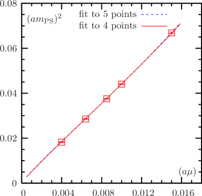
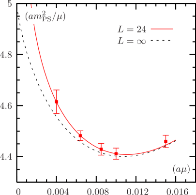
Figure 3: Left: $(am_{\pi})^{2}$ as a function of the twisted mass $a\mu$; right: $(am_{\pi})^{2}/(a\mu)$ versus $a\mu$ (by the ETM Collaboration). The finite volume ChPT-fit is shown, together with the infinite volume limit (dashed line): $\bar{l}_{3}=3.65(12)$.

As examples of the results, Chiral Perturbation Theory (ChPT) fits of the pseudoscalar- (pion-) mass (in Figure 3) and pseudoscalar- (pion-) decay constant (in Figure 4) are shown. It is remarkable that the precision on $\bar{l}_{3,4}$ is much higher than obtained by any previous experimental determination. However: this is with only $N_{f}=2$ degenerate dynamical quarks ($u$- and $d$-quark) and no continuum limit extrapolation is yet performed (it is comming soon).

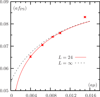
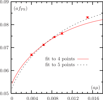
Figure 4: ChPT fits to $af_{\pi}$ versus $a\mu$ (by the ETM Collaboration). Left: the point with largest $a\mu$ left out (the dashed line is the infinite volume limit); right: compared to finite volume fit to every point. The fit gives: $a=0.087(1){\rm\,fm}$, $a^{-1}=2264(26){\rm\,MeV}$), $\;\;\bar{l}_{4}=4.52(06)$.

4.1.3 Ratio tests of PQChPT

Taking ratios at fixed gauge coupling ($\beta$) is advantageous because the Z-factors of mutiplicative renormalization cancel (for instance, in $m_{q}$ and $f_{\pi}$). Also: some types of lattice artifacts may cancel.

In case of simulations with Wilson-type lattice actions, by taking into account lattice artifacts in the Chiral Lagrangian, one can reach the continuum limit faster. This approach is based on the effective continuum theory introduced by Symanzik [4]: cutoff effects (in the lattice regularized theory) can be described by ${\cal O}(a,a^{2},\ldots)$ terms in a local effective Lagrangian.

This idea can be applied to low energy LQCD [33, 34]. In case of the Wilson quark action the leading ${\cal O}(a)$ effects have a simple chiral transformation property, identical to those of the quark masses. At leading order of ChPT, besides the quark mass variable $\chi$, an additional ${\cal O}(a)$ parameter $\rho$ appears:

$$\chi\equiv\frac{2B_{0}m_{q}}{f_{0}^{2}}\ ,\hskip 30.00005pt\rho\equiv\frac{2W_{0}a}{f_{0}^{2}}\hskip 40.00006pt\left(\eta\equiv\frac{\rho}{\chi}\right)\ .$$ (113)

At next to leading order (NLO): the Gasser-Leutwyler constants $L_{1},\ldots,L_{8}$ are doubled by the (bare parameter dependent) coefficients $W_{1},\ldots,W_{8}$ describing ${\cal O}(a)$ effects. (Extension to ${\cal O}(a^{2})$ is possible.)

Variables to be used in ratio tests of PQChPT (the index $V$ always stands for “valence” quarks which are “quenched”, $S$ for dynamical “sea” quarks):

$$\xi\equiv\frac{m_{qV}}{m_{qS}}=\frac{\chi_{V}}{\chi_{S}}\ ,\hskip 30.00005pt\eta_{S}\equiv\frac{\rho_{S}}{\chi_{S}}\ ,\hskip 30.00005pt\sigma_{i}\equiv\frac{m_{qS}^{(i)}}{m_{qS}^{(R)}}=\frac{\chi_{S}}{\chi_{R}}\ .$$ (114)

For the pion decay constants the appropriate ratios are:

$$Rf_{VV}\equiv\frac{f_{VV}}{f_{SS}}\ ,\hskip 30.00005ptRf_{VS}\equiv\frac{f_{VS}}{f_{SS}}\ ,\hskip 30.00005ptRRf\equiv\frac{f_{VS}^{2}}{f_{VV}f_{SS}}\ ,$$ (115)

and for the pion mass-squares (dividing by the leading order behaviour):

$$Rn_{VV}\equiv\frac{m_{VV}^{2}}{\xi m_{SS}^{2}}\ ,\hskip 20.00003ptRn_{VS}\equiv\frac{2m_{VS}^{2}}{(\xi+1)m_{SS}^{2}}\ ,\hskip 20.00003ptRRn\equiv\frac{4\xi m_{VS}^{4}}{(\xi+1)^{2}m_{VV}^{2}m_{SS}^{2}}\ .$$ (116)

For the sea quark mass dependence

$$Rf_{SS}\equiv\frac{f_{SS}}{f_{RR}}\ ,\hskip 40.00006ptRn_{SS}\equiv\frac{m_{SS}^{2}}{\sigma m_{RR}^{2}}$$ (117)

are appropriate.

Examples of the NLO formulas are [34, 35]: for $N_{s}$ degenerate sea quarks

$$Rf_{VV} = 1+4(\xi-1)\chi_{S}L_{S5}+\frac{N_{s}\chi_{S}}{32\pi^{2}}(1+\eta_{S})\log(1+\eta_{S})$$ (118)

$$-\frac{N_{s}\chi_{S}}{64\pi^{2}}(1+\xi+2\eta_{S})\log\frac{1+\xi+2\eta_{S}}{2}\ ,$$

$$RRf = 1+\frac{\chi_{S}}{32N_{s}\pi^{2}}(\xi-1)-\frac{\chi_{S}}{32N_{s}\pi^{2}}(1+\eta_{S})\log\frac{\xi+\eta_{S}}{1+\eta_{S}}\ ,$$ (119)

$$Rf_{SS} = 1+4(\sigma-1)\chi_{R}(N_{s}L_{R4}+L_{R5})+4(\eta_{S}\sigma-\eta_{R})\chi_{R}(N_{s}W_{R4}+W_{R5})$$ (120)

$$-\frac{N_{s}\chi_{R}}{32\pi^{2}}\sigma(1+\eta_{S})\log[\sigma(1+\eta_{S})]+\frac{N_{s}\chi_{R}}{32\pi^{2}}(1+\eta_{R})\log(1+\eta_{R})\ ,$$

and similarly for $Rn\ldots$.

In the above formulas $L_{Sk}$ denote Gasser-Leutwyler constants renormalized at the scale $f_{0}\sqrt{\chi_{S}}$. They are related to $\bar{L}_{k}$ defined at the scale $f_{0}$ and $L^{\prime}_{k}$ defined at the generic scale $\mu$ according to

$$L_{Sk}=\bar{L}_{k}-c_{k}\log(\chi_{S})=L^{\prime}_{k}-c_{k}\log(\frac{f_{0}^{2}}{\mu^{2}}\chi_{S})\ ,$$ (121)

with some (known) constants $c_{k}$. The corresponding relations for the coefficients $W_{Sk}$ are:

$$W_{Sk}=\bar{W}_{k}-d_{k}\log(\chi_{S})=W^{\prime}_{k}-d_{k}\log(\frac{f_{0}^{2}}{\mu^{2}}\chi_{S})\ .$$ (122)

Note that these formulas can be extended to the NNLO order, too.

A first comparison of these formulas with numerical Monte Carlo results has been performed by the qq+q Collaboration (DESY-Münster) [35]. The lattice sizes were $16^{4}$ and $16^{3}\cdot 32$, and $N_{s}=2$ light quark flavours were simulated. The lattice spacing was: $a=0.189(5)\,{\rm fm}\simeq(1.04\,{\rm GeV})^{-1}\;$ giving lattice extensions $L\simeq 3\,{\rm fm}$. The pion masses were: $am_{\pi}=0.6747(14),\;0.6211(22),\;0.4354(68),\;0.3676(23)$ which correspond in physical units to $m_{\pi}\simeq 702,\;646,\;452,\;415\,{\rm MeV}$. The sea quark masses were approximately $60\,{\rm MeV}$ to $25\,{\rm MeV}$; and the valence quark masses: $\frac{1}{2}m_{sea}\leq m_{valence}\leq 2m_{sea}$. Being the first exploratory study, the parameters did not correspond to the latest best ones, in particular, the lattice spacing was rather coarse and the quark masses not small enough.

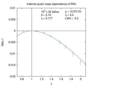
Figure 5: Numerical results of the qq+q Collaboration on $16^{3}\cdot 32$ lattice at ($\beta=5.1,\,\kappa=0.177$): one parameter fit of $(RRn-1)=\chi_{S}(1-\xi+\log\xi)/(32\pi^{2})$ (“pure chiral log“).

The result of this first study was that the formulas like (118)-(120) describe well the dependence on both sea and valence quark masses, in particular if some generic NNLO terms are included. As an example of the fits see Figure 5. First crude estimates of L-G constants, renormalized at scale $f_{0}\sqrt{\chi_{R}}$, gave with $\chi_{R}=33.5(2.4)$

$$L_{R5}=3.00(19)\cdot 10^{-3}\ ,\hskip 30.00005pt(2L_{R8}-L_{R5})=-6.25(52)\cdot 10^{-4}\ .$$ (123)

From the sea quark mass dependence it was obtained

$$(2L_{R4}+L_{R5}) = 4.34(28)\cdot 10^{-3}\ ,$$

$$(4L_{R6}+2L_{R8}-2L_{R4}-L_{R5}) = -9.1(6.4)\cdot 10^{-5}\ ,$$

$$\frac{\Lambda_{3}}{f_{0}} = 6.51(57)\ ,$$

$$\frac{\Lambda_{4}}{f_{0}} = 22.9(1.5)$$ (124)

These numnbers can only be taken as crude estimates, because they come from a point with coarse lattice spacing and no continuum extrapolation has been performed.

5 Outlook

The present goal of numerical Monte Carlo investigations is to perform dynamical quark simulations with light quarks in large volumes. After about twenty-thirty years of hard work – which can be considered as the preparation – the presently available computer resources and algorithmic developments make this goal achievable. The big question is, can we validate QCD as the true theory of strong interactions by comparing the results with experimental knowledge? After this will be done, lattice gauge theorists will be able to extend their research area to study at the non-perturbative level a broader class of Quantum Field Theories not just QCD.

5.1 Beyond QCD

The further development of lattice regularized Quantum Field Theories will reflect how the two basic theoretical problems of the Electroweak Standard Model will be resolved in a “beyond the Standard Model” framework. These two problems are:

• The triviality of the Higgs-Yukawa sector: as a consequence of appearance of Landau-Pomeranchuk poles there are cut-off dependent upper bounds on the Higgs- and Yukawa-couplings, which tend to zero for infinite cut-off (i.e. zero lattice spacing).

• It is very difficult to define chiral gauge theories in lattice regularization – although they are required for the electroweak sector. Mirror fermion states with opposite chirality appear and it is difficult to separate the mass scale of the mirror fermion sector from the known chiral sector [36]. By including the mirror fermion sector the theory becomes vector-like (non-chiral).

These problems become acute at the TeV scale and need some solution in a near future – in particular based on the experimental input expected from LHC. There are several ways how these problems could perhaps be solved:

1. Supersymmetric extensions of the Standard Model: the improvement of the divergence structure due to supersymmetry (the solution of the “hierarchy problem” because of the absence of quadratic divergences) may solve both of the above problems. The mirror states could perhaps be shifted to the grand unification scale.

2. Technicolor-type models based on some appropriate generalization of QCD may produce the low-energy chiral spectrum as bound states. The mirror fermions could be at the technicolor scale.

3. Beyond QFT models where more dimensions beyond four appear and/or quantum gravity effects play an important role already near the TeV scale.

Which one (if any) of these ways is realized in Nature is a very exciting question and will hopefully become clear in the not very far future. If possibility 1. is realized then lattice field theorists will have to work more on (at least partly) supersymmetric non-perturbative regularization schemes. The case of possibility 2. seems to be a more or less straightforward generalization of QCD. In case of 3. one probably has to abandon the traditional QFT framework and look for radically new approaches.

Acknowledgments

It is a pleasure to thank the organizers, the lecturers and the students of the Spring School on High Energy Physics in Jaca, Spain for the lively and inspiring atmosphere at the School.

References

- [1] I. Montvay, G. Münster, Quantum Fields on a Lattice, Cambridge University Press, 1994.
- [2] K.G. Wilson, Phys. Rev. D 10 (1974) 2445.
- [3] K. G. Wilson and J. B. Kogut, Phys. Rept. 12 (1974) 75.
- [4] K. Symanzik, Nucl. Phys. B 226 (1983) 187.
-
[5]
P. Weisz,
Nucl. Phys. B 212 (1983) 1.
P. Weisz and R. Wohlert, Nucl. Phys. B 236 (1984) 397 [Erratum-ibid. B 247 (1984) 544]. - [6] Fermilab Lattice, MILC and HPQCD Collaboration, A.S. Kronfeld et al., PoS LAT2005 (2005) 206, Int. J. Mod. Phys. A21 (2006) 713; hep-lat/0509169.
- [7] R. Frezzotti, P. A. Grassi, S. Sint and P. Weisz, Nucl. Phys. Proc. Suppl. 83 (2000) 941; hep-lat/9909003.
- [8] R. Frezzotti and G.C. Rossi, Nucl. Phys. Proc. Suppl. 128 (2004) 193; hep-lat/0311008.
- [9] R. Frezzotti and G.C. Rossi, JHEP 0408 (2004) 007; hep-lat/0306014;
- [10] D. B. Kaplan, Phys. Lett. B 288 (1992) 342; hep-lat/9206013.
- [11] R. Narayanan and H. Neuberger, Phys. Lett. B 302 (1993) 62; hep-lat/9212019.
- [12] Y. Shamir, Nucl. Phys. B 406 (1993) 90; hep-lat/9303005.
- [13] P. H. Ginsparg and K. G. Wilson, Phys. Rev. D 25 (1982) 2649.
- [14] M. Luscher, Phys. Lett. B 428 (1998) 342; hep-lat/9802011.
- [15] P. Hasenfratz, Nucl. Phys. Proc. Suppl. 63 (1998) 53; hep-lat/9709110.
- [16] Y. Kikukawa, H. Neuberger and A. Yamada, Nucl. Phys. B 526 (1998) 572; hep-lat/9712022.
- [17] P. Hasenfratz, V. Laliena and F. Niedermayer, Phys. Lett. B 427 (1998) 125; hep-lat/9801021.
-
[18]
H. B. Nielsen and M. Ninomiya,
Nucl. Phys. B 185 (1981) 20
[Erratum-ibid. B 195 (1982) 541].
H. B. Nielsen and M. Ninomiya, Nucl. Phys. B 193 (1981) 173. - [19] P. Hernandez, K. Jansen and M. Luscher, Nucl. Phys. B 552 (1999) 363; hep-lat/9808010.
- [20] M. Golterman and Y. Shamir, Phys. Rev. D 68 (2003) 074501; hep-lat/0306002.
- [21] C. Morningstar, hep-lat/0702020.
- [22] N. Metropolis, A.W. Rosenbluth, M.N. Rosenbluth, A.H. Teller and E. Teller, J. Chem. Phys., bf 21 (1953) 1087,
- [23] D. H. Weingarten and D. N. Petcher, Phys. Lett. B 99 (1981) 333.
- [24] S. Duane, A.D. Kennedy, B.J. Pendleton, D. Roweth, Phys. Lett. B195 (1987) 216.
-
[25]
R. Frezzotti and K. Jansen,
Phys. Lett. B 402 (1997) 328; hep-lat/9702016.
R. Frezzotti and K. Jansen, Nucl. Phys. B 555 (1999) 395; hep-lat/9808011.
R. Frezzotti and K. Jansen, Nucl. Phys. B 555 (1999) 432; hep-lat/9808038. -
[26]
I. Montvay and E. Scholz,
Phys. Lett. B 623 (2005) 73; hep-lat/0506006.
E. E. Scholz and I. Montvay, PoS LAT2006 (2006) 037; hep-lat/0609042. - [27] M. A. Clark and A. D. Kennedy, Phys. Rev. Lett. 98 (2007) 051601; hep-lat/0608015.
- [28] R. Frezzotti and K. Jansen, Nucl. Phys. Proc. Suppl. 63 (1998) 943; hep-lat/9709033.
- [29] S. Weinberg, Physica A 96 (1979) 327.
- [30] J. Gasser and H. Leutwyler, Annals Phys. 158 (1984) 142.
- [31] C. W. Bernard and M. F. L. Golterman, Phys. Rev. D 49 (1994) 486; hep-lat/9306005.
- [32] Ph. Boucaud et al. [ETM Collaboration], hep-lat/0701012.
- [33] S. R. Sharpe and R. L. . Singleton, Phys. Rev. D 58 (1998) 074501; hep-lat/9804028.
- [34] G. Rupak and N. Shoresh, Phys. Rev. D 66 (2002) 054503; hep-lat/0201019.
-
[35]
F. Farchioni, C. Gebert, I. Montvay, E. Scholz and L. Scorzato [qq+q
Collaboration],
Phys. Lett. B 561 (2003) 102; hep-lat/0302011.
F. Farchioni, I. Montvay, E. Scholz and L. Scorzato [qq+q Collaboration], Eur. Phys. J. C 31 (2003) 227; hep-lat/0307002.
F. Farchioni, I. Montvay and E. Scholz [qq+q Collaboration], Eur. Phys. J. C 37 (2004) 197; hep-lat/0403014. - [36] I. Montvay, Phys. Lett. B 199 (1987) 89.