Sound speed of a Bose-Einstein condensate in an optical lattice

Abstract

The speed of sound of a Bose-Einstein condensate in an optical lattice is studied both analytically and numerically in all three dimensions. Our investigation shows that the sound speed depends strongly on the strength of the lattice. In the one-dimensional case, the speed of sound falls monotonically with increasing lattice strength. The dependence on lattice strength becomes much richer in two and three dimensions. In the two-dimensional case, when the interaction is weak, the sound speed first increases then decreases as the lattice strength increases. For the three dimensional lattice, the sound speed can even oscillate with the lattice strength. These rich behaviors can be understood in terms of compressibility and effective mass. Our analytical results at the limit of weak lattices also offer an interesting perspective to the understanding: they show the lattice component perpendicular to the sound propagation increases the sound speed while the lattice components parallel to the propagation decreases the sound speed. The various dependence of the sound speed on the lattice strength is the result of this competition.

I Introduction

A Bose-Einstein condensate(BEC) in an optical lattice has attracted great interests recently, both experimentally and theoreticallyMorschRev ; Bloch . The presence of the lattice can remarkably enrich the behaviors of the system compared to the uniform case, providing a new fertile ground for exploring a variety of solid-state effects in BECs, for example, Bloch oscillationsAnderson ; Morsch ; Choi and Landau-Zener tunnelingLoop1 ; Zobay ; Jona ; Loop2 between Bloch bands in an accelerating optical lattice. Moreover, a BEC in an optical lattice can be considered as quantum simulators and therefore used for testing fundamental theoretical conceptsBloch . For example, it can be used to simulate the Bose-Hubbard model and study experimentally the quantum phase transition between superfluid and Mott-insulatorJaskch ; Greiner .

In this article, we launch a systematic study of the speed of sound for a BEC in an optical lattice in all three dimensions. The speed of sound is important for two simple reasons: (1) it is a basic physical parameter that tells how fast the sound propagates in the system; (2) it is intimately related to superfluidity according to Landau’s theory of superfluid. Because of these, the sound propagation and its speed was one of the first things that have been studied by experimentalists on a BEC since its first realization in 1995BEC1995 . The propagation of sound in a harmonically trapped condensate without the lattice has already been observed experimentallyAndrews and studied theoreticallyZaremba . Now there are experimental efforts to measure the sound speed for a BEC in an optical latticeDu .

There have been a great deal of theoretical work done to understand the sound speed for a BEC in an optical lattice. These studies show that three parameters strongly affect the speed of sound: the strength of the optical lattice $v$, the interaction between atoms $c$, and the lattice dimension $D$ ($D=1,2,3$). In Ref.Berg , the phonon excitations of the BECs in one-dimensional optical lattice ($D=1$) are theoretically investigated by solving the Bogoliubov equations. Their analytic results for the sound speed in the weak potential limit predicted that the sound speed decreases monotonically with increasing the depth of the optical lattice. The most detailed study of sound propagation in one-dimensional lattice was done by Pitaevskii and Stringari’s groupKraer ; Menotti , who also found the sound speed is suppressed by the lattice. In particular, Ref. Kraer presents the detailed comparison between the sound speed obtained by Bogoliubov theory with the one obtained from the compressibility and the effective mass. Similar resultsDanshita were also obtained for the Krönig-Penney potential, a special form of the periodic potential. Furthermore, Martikainen and StoofMartikainen examined the effect of the transverse breathing mode on the longitudinal sound propagation for a BEC in a one-dimensional optical lattice. In particular, they discuss how the coupling with the transverse breathing mode influences the sound velocity in an optical lattice. Krämer et al.Kramer also studied the effect of the transverse degrees of freedom on the velocity of sound of a BEC in 1D optical lattice and radially confined by a harmonic trap. A recent paper by Taylor and ZarembaTaylor studied the Bogoliubov excitations of a BEC in an optical lattice in all spatial dimensions. However, the formulation in Ref. Taylor is in principle; the authors did not present the concrete results of sound speed in two and three-dimensional cases(D=2,3). Most interestingly, with numerical calculations Boers et al.Boers found that the sound speed of a BEC in a three-dimensional optical lattice achieves a maximum with increasing lattice depth. Because of the difficulty to obtain the Bloch states with interaction, the investigation of Boers et al. is limited to the low density so that the Bloch wave function of the free particle can be used as an approximation.

Our investigation here tries to overcome the deficiencies in previous studies to give a complete picture how the sound speed is affected by the lattice strength $v$, the interaction between atoms $c$, and the dimensionality $D$. Analytical approaches are used in two limiting cases: weak lattice and strong lattice. For weak lattices, they can be viewed as perturbations. In this case, we obtain an analytical expression to the second order of the lattice strength for the sound speed of a BEC in an arbitrary periodic potential. We have analyzed this result for the important case of the periodic potential being an optical lattice. Our analysis finds a strong dependence of the sound speed on the lattice dimensions. Especially, we find that the lattice component perpendicular to the sound propagation increases the sound speed while the lattice components parallel to the propagation suppresses the sound speed. Since the lattice can only be parallel to the propagation direction of sound in one dimension ($D=1$), the sound speed falls monotonically with increasing lattice strength. In two and three dimensions ($D=2,3$), there are both perpendicular and parallel components in the lattice and, therefore, there is a competition. As a result, there is a rich dependence of the sound speed on lattice strength in the case of $D=2,3$. The sound speed can first increases then decreases as the lattice strength increases. We have also tried to understand these results from a different angle, i.e., in terms of compressibility $\kappa$ and effective mass $m^{*}$. The analytical expression is found for compressibility $\kappa$ and effective mass $m^{*}$ for a BEC in an optical lattice. We find that the effect of the lattice on the sound speed reflects a competition between the slowly decreasing compressibility $\kappa$, and the increasing effective mass $m^{*}$, with increasing lattice depth.

In the limit of strong lattices, it is reasonable to use the tight-binding model to describe the BEC in an optical latticeSmerzi . Our analytical results display that the sound speed always exponentially decreases with increasing the optical lattice in all dimensions. This $D$-independent behavior of sound speed can be understood as the competition between the tunneling strength $J$ between adjacent sites and the interaction $U$ between the atoms at a lattice site. With increasing lattice depth, $U$ slowly increases while $J$ exponentially decreases, resulting in monotonically decreasing speed of sound.

Our analytical results are complemented by our numerical study, where the results are obtained for all ranges of lattice strength. Our numerical results agree well with our analytical results in both weak potential and tight-binding limits for the case of weak interatomic interaction. For the intermediate strength of lattice, we find that the sound speed even oscillates with the lattice strength for a three-dimensional optical lattice. We emphasize that in our numerical calculations the interaction between atoms is taken into account to compute the Bloch states in all three dimensions. In Ref.Boers , the interaction is neglected in computing Bloch states for BECs and the Bloch states of free bosons were used as an approximation.

This paper is organized as follows. In Section II, for the sake of self-containment and introducing notations, we describe the basic theoretical framework of our study. It includes the definition of the sound speed $v_{s}$, compressibility $\kappa$, and effective mass $m^{*}$. In Section III, we present the analytic results of the sound speed for a BEC in the optical lattice in both weak potential limit and tight-banding regime. Section IV contains our numerical study of the sound speed. The details of our numerical methods are given here. In Section V, we discuss the possibility of observing the phenomena presented in this paper within the current experimental capability. The last section (Sec. VI) contains a discussion of our results and concluding remarks. Five appendices are given at the end to show the detailed steps to derive our key analytical results in the main text.

II Basic theory

II.1 Mean-field theory of Bose-Einstein condensates

We focus on the situation that the BEC system can be well described by the mean-field theory. In this case, the BEC system is governed by the following grand-canonical Hamiltonian,

$$\mathscr{H} = \int d^{3}\vec{r}\Big{\{}\psi^{*}\left(\vec{r}\right)\Big{[}-\frac{1}{2}\nabla^{2}+V_{latt}\left(\vec{r}\right)\Big{]}\psi\left(\vec{r}\right)$$ (1)

$$+\frac{c}{2}\left|\psi\left(\vec{r}\right)\right|^{4}-\mu\left|\psi\left(\vec{r}\right)\right|^{2}\Big{\}}.$$

In our case, the external potential is a three-dimensional optical lattice created by six laser beams that are perpendicular to each otherMorschRev ; Bloch ,

$$V_{latt}\left(\vec{r}\right)=v\Big{[}\cos\left(x\right)+\cos\left(y\right)+\cos\left(z\right)\Big{]},$$ (2)

where $v$ characterized the strength of the optical lattice. In Eq. (1), all the variables are scaled to be dimensionless by the system’s basic parameters: the atomic mass $m$, the wave number $k_{L}$ of the laser light, and the average density $n_{0}$. The chemical potential $\mu$ and the strength $v$ of the periodic potential are in the units of $4\hbar^{2}k_{L}^{2}/m$, the wave function $\psi$ is in the units of $\sqrt{n_{0}}$, $\vec{r}$ is in the units of $1/2k_{L}$, and t is the units of $m/4\hbar k_{L}^{2}$. The nonlinear coefficient $c=\pi n_{0}a_{s}/k_{L}^{2}$, where $a_{s}>0$ is the $s$-scattering length.

Sound is a propagation of small density fluctuations inside a system. To study sound in a BEC, one first need to find out the ground state of this BEC system, which serves as a media for sound propagation. The sound speed can then be found by perturbing the ground state as explained in detail in the next subsection.

The ground state of a BEC in an optical lattice is a Bloch state at the center of the Brillouin zone. Briefly, the Bloch state is of the following form

$$\psi(\vec{r})=e^{i\vec{k}\cdot\vec{r}}\phi_{\vec{k}}(\vec{r}),$$ (3)

where $\vec{k}$ is the Bloch wave vector and $\phi_{\vec{k}}\left(\vec{r}\right)$ is a periodic function with the same periodicity of the optical lattice. The Bloch wave function $\phi_{\vec{k}}(\vec{r})$ satisfies the following stationary Gross-Pitaevskii equation

$$-\frac{1}{2}\left(\nabla+i\vec{k}\right)^{2}\phi_{\vec{k}}+c|\phi_{\vec{k}}|^{2}\phi_{\vec{k}}+V_{latt}\left(\vec{r}\right)\phi_{\vec{k}}=\mu(\vec{k})\phi_{\vec{k}},$$ (4)

where $\mu(\vec{k})$ is the chemical potential. The energy of the system in a Bloch state is given by

$$E\left(\vec{k}\right)=\int d^{3}\vec{r}\Big{\{}\phi^{*}_{\vec{k}}\big{[}-\frac{\left(\nabla+i\vec{k}\right)^{2}}{2} + V_{latt}\left(\vec{r}\right)\big{]}\phi_{\vec{k}}$$ (5)

$$+ \frac{c}{2}\left|\phi_{\vec{k}}\right|^{4}\Big{\}}.$$

The set of energies $E(\vec{k})$ then forms a Bloch bandWu ; Smith . The Bloch state can be obtained analytically in certain circumstancesExact . In most cases, it has to be computed numericallyWu ; Seaman . The numerical method of this study is described in Section VI. To compute the sound speed, one may only need the Bloch state $\phi_{0}$ at $\vec{k}=0$. However, for the effective mass defined by

$$\frac{1}{m^{*}}=\frac{\partial^{2}E\left(\vec{k}\right)}{\partial k^{2}},$$ (6)

where $k=|\vec{k}|$, one also has to compute Bloch states in the vicinity of $\vec{k}=0$. In this article, we also study one- and two-dimensional cases. The one-dimensional optical lattice is given by

$$V(x)=v\cos(x)\,,$$ (7)

and the two-dimensional optical lattice is given by

$$V(x,y)=v[\cos(x)+\cos(y)]\,.$$ (8)

II.2 Definitions of the sound speed

In Section II.A, the BEC system is regarded as a Hamiltonian system by the grand canonical Hamiltonian (1); the corresponding Gross-Pitaevskii equation can be obtained by the variation of the Hamiltonian, $i\partial\psi/\partial t=\delta H/\delta\psi^{*}$,

$$i\frac{\partial\psi}{\partial t}=-\frac{1}{2}\nabla^{2}\psi+V\left(\vec{r}\right)\psi+c|\psi|^{2}\psi.$$ (9)

The Bogoliubov equations can be determined from the linear stability analysis of the GP equation (9). To explore a small disturbance $\delta\phi_{\vec{k}}\left(\vec{r},t\right)$ at a Bloch state $\phi_{\vec{k}}\left(\vec{r}\right)$, we write

$$\psi(\vec{r},t)=e^{i\vec{k}\cdot\vec{r}-i\mu t}\big{[}\phi_{\vec{k}}\left(\vec{r}\right)+\delta\phi_{\vec{k}}\left(\vec{r},t\right)\big{]},$$ (10)

where the disturbance can be similarly written as

$$\delta\phi_{\vec{k}}\left(\vec{r},t\right)=u_{\vec{k}}e^{i\left\{\vec{q}\cdot\vec{r}-\epsilon\left(\vec{q}\right)t\right\}}+v^{*}_{\vec{k}}e^{-i\left\{\vec{q}\cdot\vec{r}-\epsilon\left(\vec{q}\right)t\right\}}.$$ (11)

Plugging Eq. (11) into Eq. (9) and keeping only the linear terms, we arrive at the Bogoliubov equationsWu ,

$$\delta_{z}M_{\vec{k}}\left(\vec{q}\right)\begin{pmatrix}u_{\vec{k}}\cr v_{\vec{k}}\end{pmatrix}=\epsilon(\vec{q})\begin{pmatrix}u_{\vec{k}}\cr v_{\vec{k}}\end{pmatrix},$$ (12)

with

$$M_{\vec{k}}\left(\vec{q}\right)=\left(\begin{array}[]{cc}\mathscr{L}\left(\vec{k}+\vec{q}\right)&c\phi_{\vec{k}}^{2}\\ c\phi_{\vec{k}}^{\ast 2}&\mathscr{L}\left(-\vec{k}+\vec{q}\right)\end{array}\right),$$ (15)

and

$$\delta_{z}=\left(\begin{array}[]{cc}1&0\\ 0&-1\end{array}\right),$$ (18)

where $\mathscr{L}\left(\vec{q}\right)$ is defined as

$$\mathscr{L}\left(\vec{q}\right)=-\frac{1}{2}(\nabla+i\vec{q})^{2}+V\left(\vec{r}\right)-\mu+2c|\phi_{\vec{k}}|^{2}.$$ (19)

Note that $\vec{q}$ represents mode of the small perturbations and is of nature of Bloch wave vector as the matrix $M$ is periodic.

In general there are two equivalent definitions for the sound speed in a BEC. As sound can be regarded as a long wavelength response of a system to a perturbation, the sound speed can be extracted from the excitation of a BEC. According to the Bogoliubov theory, the excitation energy $\epsilon\left(\vec{q}\right)$ of the BEC in a Bloch state at $\vec{k}=0$ can be found by solving the eigenvalue problem of Eq. (12). In terms of these excitations, the sound speed of a BEC system can be defined as

$$v_{s}=\lim_{q\rightarrow 0}{\frac{\epsilon\left(\vec{q}\right)}{q}},$$ (20)

where $q=|\vec{q}|$.

The other definition arises when the BEC system is regarded as a hydrodynamics system. In this context, the sound speed in a BEC is given by the standard expressionPines ; Kraer ; Menotti

$$v_{s}=\sqrt{\frac{1}{\kappa m^{*}}},$$ (21)

where $\kappa$ is the compressibility of the BEC system and defined as

$$\kappa^{-1}=n_{0}\frac{\partial\mu}{\partial n_{0}},$$ (22)

where the chemical potential $\mu$ and $n_{0}$ is the averaged density. For a BEC system with repulsive interatomic interaction, the optical trapping reduces the compressibility of the system as the effect of the repulsion is enhanced by squeezing the condensate in each well. According to the definition of sound speed in Eq. (21), the sound speed reflects the competition between the compressibility $\kappa$ and the effective mass $m^{*}$.

Both definitions are used in our computations and they agree with each other as expected. The proof of the equivalence of these definitions can be found in Ref. Pines .

III Analytical results

III.1 Weak potential limit.

We consider first an arbitrary periodic potential $V_{ar}\left(\vec{r}\right)$ with the periodicity of $\vec{R}$,

$$V_{ar}\left(\vec{r}\right)=V_{ar}\left(\vec{r}+\vec{R}\right),$$ (23)

with

$$\vec{R}=m_{1}\vec{a}_{1}+m_{2}\vec{a}_{2}+m_{3}\vec{a}_{3},$$ (24)

where $\vec{r}$ is the position vector, $\vec{a}_{1}$, $\vec{a}_{2}$, and $\vec{a}_{3}$ are the three primitive vectors and $m_{1}$, $m_{2}$, $m_{3}$ range through all integral values. In the weak potential limit, the periodic potential $V_{ar}\left(\vec{r}\right)$ can be regarded as a perturbation. This allows us to solve both the Gross-Pitaevskii equation (4) and the Bogoliubov eigenvalue problem (12) perturbatively by expanding the wave function $\psi$ and chemical potential $\mu$ of the BEC system in the order of the weak potential,

$$\psi = \psi^{\left(0\right)}+\psi^{\left(1\right)}+\psi^{\left(2\right)}+...,$$

$$\mu = \mu^{\left(0\right)}+\mu^{\left(1\right)}+\mu^{\left(2\right)}+....,$$ (25)

where $\psi^{\left(0\right)},\mu^{\left(0\right)}$ is zeroth order of the potential strength, $\psi^{\left(1\right)},\mu^{\left(1\right)}$ first order, etc. We find that the sound velocity along a given direction indicated by a unit vector $\hat{r}$ is

$$v_{s}=\sqrt{c} + 8\sqrt{c}\sum_{\vec{n}\neq 0}\Big{\{}\frac{|\vec{n}|^{2}}{\left(4c+|\vec{n}|^{2}\right)^{3}}$$ (26)

$$- \frac{\left|\vec{n}\cdot\hat{r}\right|^{2}}{|\vec{n}|^{2}\left(4c+|\vec{n}|^{2}\right)^{2}}\Big{\}}{\mathscr{F}_{\vec{n}}}^{2}(V).$$

In the above, $\mathscr{F}_{\vec{n}}(V)$ is the Fourier coefficient of $V_{ar}\left(\vec{r}\right)$ as defined by

$$\mathscr{F}_{\vec{n}}(V)=\frac{1}{\Omega}\int_{cell}d^{3}\vec{r}V_{ar}(\vec{r})e^{-i\vec{n}\cdot\vec{r}},$$ (27)

with

$$\vec{n}=n_{1}\vec{b}_{1}+n_{2}\vec{b}_{2}+n_{3}\vec{b}_{3}$$ (28)

where $n_{j}$’s are integers and $\vec{b}_{j}$’s are the set of reciprocal primitive vectors defined by

$$\vec{a}_{i}\cdot\vec{b}_{j}=2\pi\delta_{ij}.$$ (29)

In the integration, $\Omega$ is the volume of the primitive cell and the integration is over one primitive cell. The detailed derivation of Eq. (26) can be found in the Appendix C.

The focus of this article is optical lattices as described in Eqs.(2,7,8). In this special but important case, the primitive vectors $\vec{a}_{1}$, $\vec{a}_{2}$, and $\vec{a}_{3}$ can be chosen along the directions of laser beams, $\vec{x}$, $\vec{y}$, and $\vec{z}$, respectively. Also we have $|\vec{a}_{1}|=|\vec{a}_{2}|=|\vec{a}_{3}|=2\pi$. For this case, we find from Eq.(26) that if the sound propagation direction is along the $x$-axis, the sound speed is (see also Eq. (93) in the Appendix C or Eq. (138) in the Appendix D)

$$v_{s}=\sqrt{c}+\sum_{\vec{n}\neq 0}\frac{8\sqrt{c}\Big{[}\left(n_{2}^{2}+n_{3}^{2}\right)|\vec{n}|^{2}-4cn_{1}^{2}\Big{]}}{|\vec{n}|^{2}\left(4c+|\vec{n}|^{2}\right)^{3}}{\mathscr{F}_{\vec{n}}}^{2}(V).$$ (30)

The sound speeds along the $y$-axis and $z$-axis can be found easily with permutation argument and the sound speed along a general direction is a certain combination of these three speeds.

When there is no periodic potential $V_{ar}\left(\vec{r}\right)=0$, the sound speed in Eq. (30) is reduced into $\sqrt{c}$, the sound speed for a BEC in free space, as expected. We also notice that there is no first-order correction to the sound speed due to the periodic potential. Most importantly, the analytical result in Eq. (30) reveals that the lattice component perpendicular to the sound propagation (generated by the laser beams along the $y$ and $z$-axes) increases the sound speed while the lattice components parallel to the propagation (generated by the laser beams along the $x$-axis) decreases the sound speed. As a result of this competition, the sound speed can either increase or decrease with lattice strength. This competition between the parallel and perpendicular components of the optical lattice certainly also applies to a general periodic potential if one carefully examines Eq.(26) and interprets “parallel” and “perpendicular” in a more sense.

To illustrate this more clearly, we consider a simple case where the periodic potential is a 1D optical lattice given by $V_{ex}(\vec{r})=v\cos(y)$. There are only two non-vanishing Fourier coefficients, i.e. $\mathscr{F}_{0,1,0}(V)=\mathscr{F}_{0,-1,0}(V)=v/2$. Then according to Eq. (30), the speeds of sound along the $x$, $y$ and $z$-axis read, respectively,

$$\left\{\begin{array}[]{rcl}v_{x,z}&=&\sqrt{c}\left(1+\frac{v^{2}}{2\left(2c+\frac{1}{2}\right)^{3}}\right),\\ v_{y}&=&\sqrt{c}\left(1-\frac{2cv^{2}}{\left(2c+\frac{1}{2}\right)^{3}}\right),\end{array}\right.$$ (31)

which show that with increasing the strength of the optical lattice the sound speed along the $y$-axis, parallel to the periodic lattice falls while the speeds of sound along both the $x$ and $z$-axes increase.

Now we study the BEC sound speed in optical lattices in terms of compressibility and effective mass according to the second definition of speed of sound, i.e. Eq.(21). Again we treat the weak optical lattice as a perturbation. For optical lattices of all dimensions as described in Eqs.(2,7,8), we find the chemical potential at $\vec{k}=0$

$$\mu=c-\frac{Dv^{2}}{4\left(2c+\frac{1}{2}\right)^{2}},$$ (32)

and the system energy near $\vec{k}=0$

$$E\left(k\right)=\frac{k^{2}}{2}-\frac{v^{2}}{\left(1+4c\right)^{2}\left(4k^{2}-1\right)}.$$ (33)

So, the chemical potential depends on $D$, the dimension of the lattice, while the energy $E(k)$ does not. The compressibility $\kappa$ can be calculated from the chemical potential $\mu$ via Eq.(22) and it is given by

$$\kappa^{-1}=c+\frac{Dcv^{2}}{\left(\frac{1}{2}+2c\right)^{3}}\,.$$ (34)

This shows that the compressibility $\kappa$ tends to decrease with increasing $v$ as the optical lattice localizes the BECs inside each well. Moreover, the compressibility $\kappa$ decreases faster with $v$ for higher dimensional lattices. The effective mass $m^{*}$ can be computed from $E(k)$ and it is found that

$$\frac{1}{m^{\ast}}=\left(1-\frac{2v^{2}}{\left(\frac{1}{2}+2c\right)^{2}}\right).$$ (35)

It is clear that the effective mass always increases with the lattice strength $v$. This is expected as the increased lattice strength suppresses the tunneling between neighboring wells thus increases the effective mass $m^{*}$. Interestingly, in contrast to the chemical potential $\mu$, the dependence of the effective mass on $v$ is independent of the lattice dimension $D$. As the speed of sound is defined as $v_{s}=\sqrt{1/(\kappa m^{*})}$, the compressibility $\kappa$ and the effective mass $m^{*}$ influence the sound speed in opposite directions.

Plugging both Eqs.(34) and (35) into Eq. (21), we find an analytical expressions for the sound speed of a BEC in an optical lattice up to the second order of $v$

$$v_{s}=\sqrt{c}\left(1+\frac{4(D-1-4c)}{\left(4c+1\right)^{3}}v^{2}\right)\,.$$ (36)

With simple algebra (see Eq. (146) in Appendix E), one can show that this expression is consistent with the more general formula in Eq.(30).

Eq.(36) indicates that in one dimension ($D=1$) the effective mass $m^{*}$ always wins over the compressibility $\kappa$, resulting in decreasing sound speed with the lattice strength. However, in two or three dimensions ($D=2,3$), the situation is very different. There exists a critical value of $c$, the interatomic interaction strength, beyond which the effective mass $m^{*}$ wins. Otherwise, the compressibility $\kappa$ has bigger influence on the speed of sound and the speed of sound increases as the lattice becomes stronger. The critical values are $c=1/4$ for $D=2$ and $c=1/2$ for $D=3$.

We have discussed the behavior of the speed of sound in two different languages: one in terms of perpendicular and parallel components of the periodic potential with Eq.(30) and the other in terms of effective mass $m^{*}$ and the compressibility $\kappa$. Are these two pictures consistent? The answer is yes. To see this, we re-write Eq.(30) as

$$v_{s} = \sqrt{c}+8\sqrt{c}\Big{\{}\sum_{\vec{n}\neq 0}\frac{|\vec{n}|^{2}}{(4c+|\vec{n}|^{2})^{3}}$$ (37)

$$-\sum_{\vec{n}\neq 0}\frac{n_{1}^{2}}{|\vec{n}|^{2}(4c+|\vec{n}|^{2})^{2}}\Big{\}}{\mathscr{F}_{\vec{n}}}^{2}(V).$$

By comparing it with Eqs.(34) and (35), it is apparent that the first term in the curly brackets comes from the compressibility $\kappa$ while the second term results from the effective mass $m^{*}$. This observation gives us the following picture: on the one hand, all components of the periodic potential contribute to the compressibility $\kappa$, which leads to the enhance of the sound speed; on the other hand, only component parallel to the sound propagation increases the effective mass $m^{*}$, which leads to the suppression of the sound speed. Since the effective mass $m^{*}$ always wins over $\kappa$ along the parallel direction, we come to the previous understanding: the perpendicular components increase the sound speed while the parallel one suppresses it.

III.2 Tight-binding regime

When the potential wells are sufficiently deep, the condensate is well localized at each lattice site and the following tight-binding model may become adequate to describe the BEC in an optical latticeSmerzi

$$\mathscr{H}=-J\sum_{<\vec{n},\vec{n}^{\prime}>}\left(\psi_{\vec{n}}^{*}\psi_{\vec{n}^{\prime}}+\psi_{\vec{n}^{\prime}}^{*}\psi_{\vec{n}}\right)+\frac{U}{2}\sum_{\vec{n}}|\psi_{\vec{n}}|^{4},$$ (38)

where the first summation is over all pairs of the nearest neighbors. The tunneling constant $J$, which quantifies the microscopic tunneling rate between adjacent sites, is given by

$$J=-\frac{1}{(2\pi)^{D}}\int d^{D}\vec{r}\left[\frac{1}{2}\left(\vec{\nabla}\varphi_{\vec{n}}\cdot\vec{\nabla}\varphi_{\vec{n}+1}\right)+\varphi_{\vec{n}}V\varphi_{\vec{n}+1}\right],$$ (39)

with $\varphi_{\vec{n}}$ being the wave function localized at site $\vec{n}$. The on-site interaction as given by

$$U=\frac{c}{(2\pi)^{D}}\int d^{D}\vec{r}\varphi_{\vec{n}}^{4}.$$ (40)

is a measure of the interaction between atoms at one lattice site. The ground state of this Hamiltonian is a constant wave function $\psi_{\vec{n}}=1$. Its excitation energy is given by $\epsilon(q)=2|\sin\left(q\pi\right)|\sqrt{2JU}$, which yield the sound speed via Eq.(20)

$$v_{s}=\lim_{q\rightarrow 0}\frac{\omega\left(q\right)}{q}=\sqrt{8\pi^{2}JU}\,.$$ (41)

This result is consistent with the sound speed definition in terms of compressibility $\kappa$ and effective mass $m^{*}$ since

$$J=\frac{1}{8\pi^{2}}\frac{m}{m^{*}}\,,~{}~{}~{}~{}~{}~{}U\approx\kappa^{-1}\,.$$ (42)

In the following, we try to express $J$ and $U$ in terms of $c$ and $v$. For a state well-localized at each lattice site, we can regard it as the ground state of the lattice well and describe the localized state $\varphi_{\vec{n}}$ with the ground state wave function of a harmonic oscillator. This approximation immediately leads to an estimate of $U$. We obtain

$$U=c\left(4\pi^{2}v\right)^{D/4}.$$ (43)

As $U\approx\kappa^{-1}$, this indicates that the compressibility in the tight-binding limit is very similar to the weak potential limit: it depends on the dimensionality of the lattice and decrease with $v$ in a non-exponential form.

Mathematically, the time-independent Schrödinger equation for an atom in the cosine potential is a Mathieu equation. The theory of the Mathieu equation allows us to estimate $J$, which is given byZwerger ; Abramowitz

$$J=\frac{4}{\sqrt{\pi}}v^{3/4}\exp\left[-8\sqrt{v}\right].$$ (44)

This result is very different from the weak potential limit: the effective mass $\frac{m^{*}}{m}=\frac{1}{8\pi^{2}J}$ increases exponentially with $\sqrt{v}$. As a result, $J$ should dominate the behavior of the speed sound. Combining Eq.(43) and Eq.(44), we arrive at

$$v_{s}=2^{5/2}\pi^{3/4}c^{1/2}(4\pi^{2}v)^{D/8}v^{3/8}\exp(-4\sqrt{v}),$$ (45)

which shows the speed of sound decreases monotonically with $v$ in an exponential form in all three dimensions. The sound speed in the tight-binding limit has a weak dependence on the dimension $D$ of the lattice as $D$ only appears in the prefactor of the exponential.

IV Numerical results

We have so far studied analytically the sound speed of a BEC in an optical lattice. In this section, we study the sound speed with numerical methods. Our numerical method allows us to find the sound speed for the whole range of lattice strength, particularly, intermediate lattice strength for which no apparent analytical approach can be found.

IV.1 Numerical methods

As discussed in Section II, to compute the sound speed, one has to first find the ground state of the BEC system or the Bloch states in the vicinity of $\vec{k}=0$. To find these states numerically, we expand the Bloch states in Fourier series

$$\phi_{\vec{k}}(\vec{r})=\sum_{m,n,l=-N}^{N}a_{m,n,l}e^{i\left(mx+ny+lz\right)},$$ (46)

where $N$ is the cut-off. We find that $N=5$ is good enough for all dimensions. The Fourier coefficients $\{a_{m,n,l}\}$ satisfy the normalization condition

$$\sum_{m,n,l=-N}^{N}|a_{m,n,l}|^{2}=1.$$ (47)

Note that the Fourier coefficients $\{a_{m,n,l}\}$ can be chosen as real. This fact greatly reduces the computation burden.

The Bloch waves can be numerically obtained by varying $\{a_{m,n,l}\}$ so that the wave function $\phi_{\vec{k}}$ minimizes the system energy of Eq.(5); the accuracy is checked by substituting the solutions into the Gross- Pitaevskii equation (4). We use the standard minimization routine of MATLAB. The accuracy of the numerical solutions can be checked by substituting the numerical solutions into the time-independent Gross-Pitaevskii Eq.(4). Once the Bloch states $\phi_{\vec{k}}(\vec{r})$ have been obtained, we can compute the sound speed in two different methods. In one method, we calculate the Bogoliubov excitations $\varepsilon(q)$ of the ground state $\phi_{0}(\vec{r})$ and find the sound speed of the BEC through Eq. (20). In the other method, we can calculate the effective mass $m^{*}$ and compressibility $\kappa$, respectively, with Eqs.(6) and (22). Then the sound speed can be computed via Eq. (21). We have calculated the sound speeds with both methods and the agreement is excellent as expected.

IV.2 Results and discussion

We have computed numerically the sound speeds for all three dimensions for a wide range of lattice strength $v$ and inter-atomic interaction $c$. The results are plotted in Figs.1,2 & 3, respectively. Fig. 1 displays the sound speed in the one-dimensional case, which falls monotonically with increasing lattice strength. This is in agreement of previous studiesBerg ; Kraer ; Menotti .

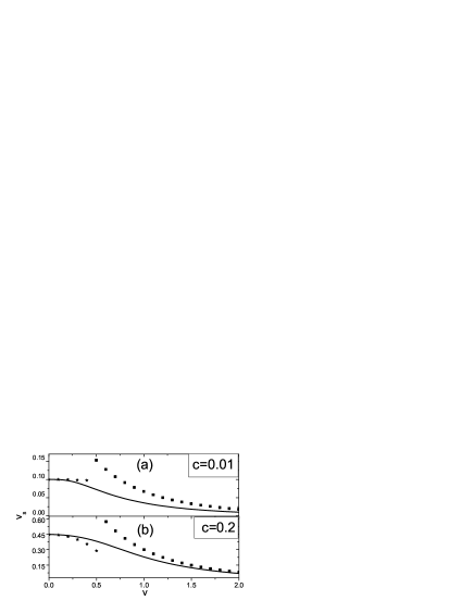
Figure 1: Sound speed for a BEC in a 1D optical lattice via the strength of the optical lattice. (i) numerical result (solid line curve); (ii) analytical results for weak potentials ($\star$ curve); (iii) analytical tight-binding results($\blacksquare$ curve).

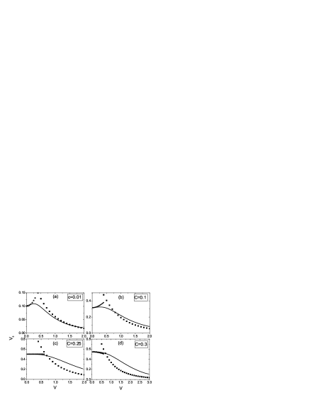
Figure 2: Sound speed for a BEC in a 2D optical lattice via the strength of the optical lattice. (i) numerical result (solid line curve); (ii) analytical results for weak potentials ($\star$ curve); (iii) analytical tight-binding results($\blacksquare$ curve).

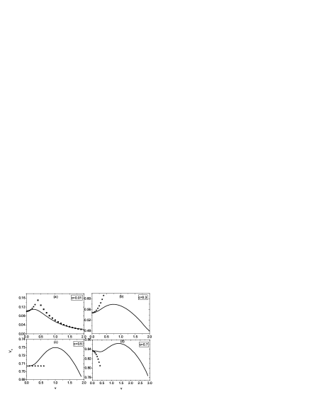
Figure 3: Sound speed for a BEC in a 3D optical lattice via the strength of the optical lattice. (i) numerical result (solid line curve); (ii)analytical results for weak potentials ($\star$ curve); (iii) analytical tight-binding results($\blacksquare$ curve).

The results are different in two and three dimensions. As shown in Figs. 2 and 3, the relationship between the sound speed and the lattice strength depends crucially on the strength of interatomic interaction. In the two-dimensional case, when the interaction is above the critical value, i.e. $c>\frac{1}{4}$, the speed of sound also decreases monotonically with increasing lattice strength (Fig.2(d)). However, when the interaction is weak, i.e. $c<\frac{1}{4}$, as shown in Fig. 2(a,b), a sound speed reaches a maximum at an intermediate strength of optical lattice. Fig.2(c) shows the transition point between the above two different behaviors, where the sound speed changes almost does not change with weak lattice potentials.

In three dimensions, the behavior becomes even richer. There exists a critical value of the interatomic interaction, $c=\frac{1}{2}$. When the interaction is smaller than this critical value $c<\frac{1}{2}$, the sound speed first increases then decreases as the lattice strength increases (Fig. 3(a,b,c)). This is similar to the two-dimensional case and was first noticed by Boers et al.Boers . However, when the interaction is strong enough, i.e. $c>\frac{1}{2}$, a new pattern is found. As shown in Fig. 3(d), the sound speed can even oscillate with the lattice strength. According to our numerical results, the oscillating behavior of the sound speed does not disappear until the interatomic interaction $c$ reaches 1 ($c=1$).

Our numerical results are compared to our analytical results. As seen in Figs. 1, 2 and 3, our numerical results agree very well with our analytical results($\star$ curves) in the regime of weak potentials. For strong lattices, our numerical results also agree well with the tight-binding results ($\blacksquare$ curve in Figs. 1, 2(a) and 3(a)) for weak interactions. However, for strong interaction in two and three dimensions, there exist discrepancy between the tight-binding results and our numerical results. This discrepancy is very large especially for three dimensions as shown in Fig. 3(b,c,d). The agreement can only be best described as qualitative.

This big mismatch is nevertheless expected as both Eq.(43) and Eq.(44) are derived without the consideration of interaction between atoms. It can be explained by noticing that the interaction can strongly modify the ground state wavefunction localized in each well and greatly enhance the tunneling between the adjacent wells in two and three dimensions. As in Eq. (42), the tunneling rate $J$ is related to the effective mass $m^{*}$, which is very sensible to the behaviour of the wave function in the region of the barriers. In Figs. 4(a1)-(a2), Figs. 5(a1)-(a4) and Figs. 6(a1)-(a4), we show the effect of the interaction $c$ on the effective mass $m^{*}$. The effect is different in different dimensions. For one dimension, as shown in Figs. 4(a1)-(a2), the effective mass $m^{*}$ increases greatly with the lattice strength for both weak and strong interaction. In 2D, the interaction has much stronger influence on $m^{*}$. If we compare Fig.5(a1) and Fig.5(a4), the influence is order of magnitude different. In 3D, the interaction $c$ affect the effective mass $m^{*}$ most strongly. As shown in Fig. 6(a1), for weak interaction $c=0.01$, the effective mass increases to $\sim 150$ at $v=2$. In Fig. 6(a4) for $c=0.7$, the effective mass $m^{*}$ is only $\sim 3$ at $v=2$. This order of magnitude difference explains why there are large disagreement between our numerical results and the tight-binding model for the speed of sound in Fig.3(b-d).

The dependence of sound speeds on the lattice strength $v$ is largely expected from our analytical results for the two limiting cases of weak and strong lattices. We have shown that in the weak lattice limit, the speed of sound can either increase or decrease with the lattice strength while in the strong lattice limit the speed of sound always decreases with increasing lattice strength. Naively, one would expect that the speed of sound either decreases monotonically with the lattice strength $v$ or develops a maximum at certain intermediate value of $v$. This is exactly what we have seen in Figs. 1, 2 and 3 except in Fig.3(d) where we see two local maxima.

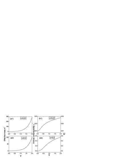
Figure 4: Inverse compressibility $\kappa^{-1}$, effective mass $m^{*}$ and on-site interaction energy $U$ for a BEC in a 1D optical lattice via the strength of the optical lattice.

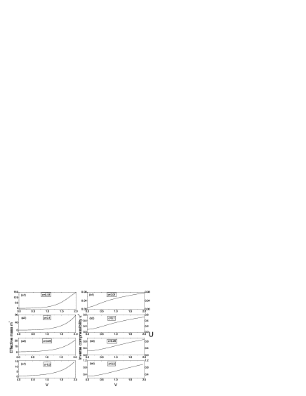
Figure 5: Inverse compressibility $\kappa^{-1}$, effective mass $m^{*}$ and on-site interaction energy $U$ for a BEC in a 2D optical lattice via the strength of the optical lattice.

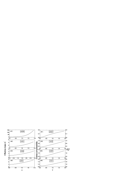
Figure 6: Inverse compressibility $\kappa^{-1}$, effective mass $m^{*}$ and on-site interaction energy $U$ for a BEC in a 3D optical lattice via the strength of the optical lattice.

To better understand the behavior of the sound speed as a function of the lattice strength $v$, we have also compute numerically the effective mass $m^{*}$ and the compressibility $\kappa$ and the results are plotted in Figs.4,5,&6. It is clear from these figures that the compressibility $\kappa$ has different dependence on $v$ in different dimensions. This agrees with our analytical results in the last section. However, we notice that the increasing rate of $\kappa^{-1}$ with $v$ is quite close in all dimensions.

The situation is different for the effective mass $m^{*}$. In the last section, we have shown that the effective mass $m^{*}$ has the same dependence on $v$ (see Eq. (35)) in all dimensions. However, it is true only in the limit of weak lattices. As seen in the right columns of Figs.4,5, &6, the effective mass $m^{*}$, as a function of $v$, behaves very differently in different dimensions. In particular, the increasing rate of $m^{*}$ with $v$ in one dimension is orders of magnitude larger than the increasing rate in three dimensions. The two-dimensional case is right in the between. Since the sound speed is the result of competition of $m^{*}$ and $\kappa$, the relatively small increasing rate of $m^{*}$ with $v$ allows the sound speed oscillates with $v$ in 3D.

V Experiments

The speed of sound of a BEC in an optical lattice may be measured with the similar technique that was used in Ref.Andrews to measure the sound speed of a BEC in a trap. Some complication is expected due to the periodic modulation of the BEC density. Another possible method is to employ Bragg spectroscopyBragg ; Excitation ; Du to the excitation spectrum. The speed of sound can be extracted from the slope of the linear part of the excitation spectrum.

In typical experiments to date, the relevant parameters are as follows: for a BEC in three-dimensional optical latticeGreiner , the atom occupancy per lattice is of the order of $\langle n_{i}\rangle\approx 1\sim 3$, $n_{0}=1.3\sim 3.9\times 10^{19}m^{-3}$, $k_{L}=2\pi/\lambda_{L}=7.37\times 10^{6}m^{-1}$, and $a_{s}=5.4nm$; for a BEC in quasi-two-dimensional optical latticeP2 , the atom occupancy per lattice can reach $\langle n_{i}\rangle\approx 170$, $n_{0}=3.6\times 10^{20}m^{-3}$, $k_{L}=2\pi/\lambda_{L}=7.37\times 10^{6}m^{-1}$, and $a_{s}=5.4nm$; for a BEC in quasi-one dimensional optical latticeP1 , $\langle n_{i}\rangle\approx 1000$, $n_{0}=2.8\times 10^{20}m^{-3}$, $k_{L}=2\pi/\lambda_{L}=7.9\times 10^{6}m^{-1}$, and $a_{s}=5.4nm$. These parameters correspond to $c=0.08$ for 1D optical lattice, $c=0.11$ for 2D optical lattice, and $c=0.004\sim 0.012$ for 3D optical lattice. The depth of optical lattice $V_{0}$ can be changed from $0E_{R}$ to $32E_{R}$Greiner ; it means that our $v$ can be changed from $0$ and $2$. To our knowledge, the highest atomic density without lattice is $n_{0}=3\times 10^{21}m^{-3}$ for sodiumInouye . For this high density, we have $c=0.22$ with $k_{L}=1.07\times 10^{7}m^{-1}$Choi . However, this is rather idealistic. The other possible way to increase $c$ is to tune the scattering length $a_{s}$ with Feshbach resonanceFesh ; FeshBloch .

VI Conclusions

We have studied the speed of sound, compressibility, and effective mass of a Bose-Einstein condensate in an optical lattice both analytically and numerically. Special attentions have been paid to the effect of the depth of the optical lattice $v$, the interatomic interaction $c$ and the dimensionality $D$ on the sound speed. Our investigation shows that the sound speed depends strongly on the strength of the lattice. In the one-dimensional case, the speed of sound falls monotonically with increasing lattice strength. The dependence becomes much richer in two and three dimensions. In the two-dimensional case, when the interaction is weak, the sound speed first increases then decreases as the lattice strength increases. For the three-dimensional case, the sound speed can even oscillate with the lattice strength. These rich behaviors can be understood in terms of competition between compressibility and effective mass. Our analytical results at the limit of weak lattices also offer an interesting perspective to the understanding: they show the lattice component perpendicular to the sound propagation decreases the sound speed while the lattice components parallel to the propagation increases the sound speed.

VII Acknowledgements

We thank X. Du and D. J. Heinzen for helpful discussion. This work is supported by the “BaiRen” program of the Chinese Academy of Sciences, the NSF of China (10504040), and the 973 project of China (2005B724500). Z. D. Zhang and Z. X. Liang is supported by the NSF of China (10674139).

Appendix A Preliminary notations

Suppose $f\left(\vec{r}\right)$ to be a periodic function with the periodicity of $\vec{R}$, given by

$$f\left(\vec{r}\right)=f\left(\vec{r}+\vec{R}\right),$$ (48)

with

$$\vec{R}=m_{1}\vec{a}_{1}+m_{2}\vec{a}_{2}+m_{3}\vec{a}_{3},$$ (49)

where $\vec{r}$ is the position vector, $\vec{a}_{1}$, $\vec{a}_{2}$, and $\vec{a}_{3}$ are any three vectors not all in the same plane, and $m_{1}$, $m_{2}$, and $m_{3}$ ranges through all integral values. Corresponding to $\vec{a}_{i}$’s, there exist a set of reciprocal vectors $\vec{b}_{j}$’s such that

$$\vec{a}_{i}\cdot\vec{b}_{j}=2\pi\delta_{ij}.$$ (50)

We can expand the periodic function $f\left(\vec{r}\right)$ as its Fourier coefficients $\mathscr{F}_{\vec{n}}(f)$ as defined by,

$$f\left(\vec{r}\right)=\sum_{\vec{n}}\mathscr{F}_{\vec{n}}\left(f\right)\exp\Big{\{}{i\vec{n}\cdot\vec{r}}\Big{\}},$$ (51)

with

$$\mathscr{F}_{\vec{n}}\left(V\right)=\frac{1}{\Omega}\int_{cell}d\vec{r}f\left(\vec{r}\right)\exp\Big{\{}-i\vec{n}\cdot\vec{r}\Big{\}},$$ (52)

and

$$\vec{n}=n_{1}\vec{b}_{1}+n_{2}\vec{b}_{2}+n_{3}\vec{b}_{3}.$$ (53)

where the $n_{j}$ are integers. In the integration, $\Omega$ is the volume of the primitive cell and the integration is over a primitive cell.

Appendix B Solutions of the Gross-Pitaevskii equation in the weak potential limit

The time-independent Gross-Pitaevskii (GP) equation in the three-dimensional case can be written as

$$-\frac{1}{2}\bigtriangledown^{2}\psi(\vec{r})+c{|\psi(\vec{r})|}^{2}\psi(\vec{r})+V_{ar}(\vec{r})\psi(\vec{r})=\mu\psi(\vec{r}),$$ (54)

where $V_{ar}(\vec{r})$ is the periodic potential with the periodicity of $\vec{R}$,

$$V_{ar}\left(\vec{r}\right)=V_{ar}\left(\vec{r}+\vec{R}\right).$$ (55)

The Bloch-wave solutions of the GP equation (54) reads

$$\psi(\vec{r})=\phi_{\vec{k}}(\vec{r})e^{i\vec{k}\cdot\vec{r}},$$ (56)

where $\vec{k}$ is the Bloch wavenumber and $\phi_{\vec{k}}(\vec{r})$ is a periodic function with the same periodicity of Eq. (55). Substituting Eq. (56) into Eq. (54), we have the following equation for each Bloch wave state $\phi_{\vec{k}}(\vec{r})$

$$-\frac{1}{2}{(\bigtriangledown+i\vec{k})}^{2}\phi_{\vec{k}}(\vec{r}) + c{|\phi_{\vec{k}}(\vec{r})|}^{2}\phi_{\vec{k}}(\vec{r})$$

$$+V_{ar}(\vec{r})\phi_{\vec{k}}(\vec{r}) = \mu\left(\vec{k}\right)\phi_{\vec{k}}(\vec{r}).$$ (57)

The set of eigenvalues $\mu(\vec{k})$ then forms Bloch bands.

Besides the GP equation (54), the Bloch wave function is also subject to the normalization condition given by

$$\frac{1}{\Omega}\int_{cell}d\vec{r}{|\phi|}^{2}=1,$$ (58)

which is equivalent to

$$\mathscr{F}_{\vec{0}}({|\phi|}^{2})=1.$$ (59)

For convenience, we have dropped the suffix $\vec{k}$ and the coordinate vector $\vec{r}$ in $\phi_{\vec{k}}\left(\vec{r}\right)$

Expanding $\phi$ in terms of the potential strength as

$$\phi=\phi^{(0)}+\phi^{(1)}+\phi^{(2)}+\cdots,$$ (60)

we get the zeroth, first, and second order forms of Eq. (59), respectively,

$${\mathscr{F}_{\vec{0}}({|\phi|}^{2})}^{(0)}=\sum_{\vec{n}}{|\mathscr{F}_{\vec{n}}(\phi^{(0)})|}^{2}=1,$$ (61)

$${\mathscr{F}_{\vec{0}}({|\phi|}^{2})}^{(1)} = \sum_{\vec{n}}\left(\mathscr{F}_{\vec{n}}(\phi^{(0)}){\mathscr{F}_{\vec{n}}^{*}(\phi^{(1)})}\right.$$ (62)

$$\left.+\mathscr{F}_{\vec{n}}(\phi^{(1)}){\mathscr{F}_{\vec{n}}^{*}(\phi^{(0)})}\right)=0,$$

$${\mathscr{F}_{\vec{0}}({|\phi|}^{2})}^{(2)} = \sum_{\vec{n}}\left(\mathscr{F}_{\vec{n}}(\phi^{(0)}){\mathscr{F}_{\vec{n}}^{*}(\phi^{(2)})}+{|\mathscr{F}_{\vec{n}}(\phi^{(1)})|}^{2}\right.$$ (63)

$$\left.+\mathscr{F}_{\vec{n}}(\phi^{(2)}){\mathscr{F}_{\vec{n}}^{*}(\phi^{(0)})}\right)=0.$$

There is still an arbitrary phase in the above wave functions, which satisfy both the GP equation and the normalization condition. Therefore, we may impose a third condition

$$\frac{1}{\Omega}\int d\vec{r}|\phi|^{2}\in\mathbb{R},$$ (64)

So that the Bloch states can be uniquely determined.

Before solving the GP equation (54), we have to set forth another two specifications. First, we are only concerned with Bloch states at $\vec{k}=0$. In this case, we rewrite Eq. (B) as follows

$$-\frac{1}{2}\bigtriangledown^{2}\phi+c{|\phi|}^{2}\phi+V_{ar}(\vec{r})\phi=\mu\phi,$$ (65)

where we dropped the suffix $\vec{0}$ and the coordinate vector $\vec{r}$ in $\phi_{\vec{0}}(\vec{r})$ for convenience. Expanding $\phi$ and $\mu$ in terms of the potential strength, we get the zeroth, first and second order forms of Eq. (65), respectively,

$$-\frac{1}{2}\bigtriangledown^{2}\phi^{(0)}+c{|\phi^{(0)}|}^{2}\phi^{(0)}=\mu^{(0)}\phi^{(0)},$$ (66)

$$-\frac{1}{2}\nabla^{2}\phi^{(1)}+c\left(2{|\phi^{(0)}|}^{2}\phi^{(1)}+{\phi^{(0)}}^{2}{\phi^{(1)}}^{*}\right)$$

$$+V_{ar}(\vec{r})\phi^{(0)}=\mu^{(0)}\phi^{(1)}+\mu^{(1)}\phi^{(0)},$$ (67)

$$-\frac{1}{2}\nabla^{2}\phi^{(2)}+c\left(2{|\phi^{(0)}|}^{2}\phi^{(2)}+{\phi^{(0)}}^{2}{\phi^{(2)}}^{*}\right.$$

$$\left.+2\phi^{(0)}{|\phi^{(1)}|}^{2}+{\phi^{(0)}}^{*}{\phi^{(1)}}^{2}\right)+V_{ar}(\vec{r})\phi^{(1)}$$

$$=\mu^{(0)}\phi^{(2)}+\mu^{(1)}\phi^{(1)}+\mu^{(2)}\phi^{(0)}.$$ (68)

Second, we are only concerned with the cases in which the external potential $V_{ar}(\vec{r})$ is symmetric in each cell, or in other words, $V_{ar}(\vec{r})$ is an even function. Combining it with the condition that $V_{ar}(\vec{r})$ is a real function, we immediately have

$$\mathscr{F}_{\vec{n}}(V)=\mathscr{F}_{-\vec{n}}(V)\in\mathbb{R}.$$ (69)

In the following, we will solve the GP equation for obtaining the normalized Bloch state at $\vec{k}=0$.

B.1 The zeroth-order correction of the GP equation

From Eq. (66), we get the zeroth-order wave function and chemical potential, respectively,

$$\phi^{(0)}=1,\quad\mu^{(0)}=c,$$ (70)

which automatically meet the normalization condition (61).

B.2 The first-order correction of the GP equation

Substituting Eq. (70) into Eq. (62), we have

$$\mathscr{F}_{\vec{0}}(\phi^{(1)})+{\mathscr{F}_{\vec{0}}^{*}(\phi^{(1)})}=0.$$ (71)

From the phase condition (64), we know that $\mathscr{F}_{\vec{0}}(\phi^{(1)})$ is a real number, and therefore

$$\mathscr{F}_{\vec{0}}(\phi^{(1)})=0.$$ (72)

Substituting Eq. (70) into Eq. (B), we have

$$\frac{1}{2}|\vec{n}|^{2}\mathscr{F}_{\vec{n}}(\phi^{(1)})+c\left(\mathscr{F}_{\vec{n}}(\phi^{(1)})+\mathscr{F}_{\vec{n}}({\phi^{(1)}}^{*})\right)$$

$$+\mathscr{F}_{\vec{n}}(V)=\mu^{(1)}\delta_{\vec{n}\vec{0}}.$$ (73)

Plugging Eq. (72) into Eq. (B.2) and letting $\vec{n}=0$, we get the first-order correction of the chemical potential

$$\mu^{(1)}=\mathscr{F}_{\vec{0}}(V).$$ (74)

Taking complex conjugates on both sides of Eq. (B.2) and replacing $-\vec{n}$ with $\vec{n}$, we obtain

$$\frac{1}{2}|\vec{n}|^{2}\mathscr{F}_{\vec{n}}({\phi^{(1)}}^{*})+c\left(\mathscr{F}_{\vec{n}}(\phi^{(1)})+\mathscr{F}_{\vec{n}}({\phi^{(1)}}^{*})\right)$$

$$+\mathscr{F}_{\vec{n}}(V)=\mu^{(1)}\delta_{\vec{n}\vec{0}}.$$ (75)

The unique solution of Eqs. (B.2) and (B.2) in the case of $\vec{n}\neq 0$ reads

$$\mathscr{F}_{\vec{n}}(\phi^{(1)})=\mathscr{F}_{\vec{n}}({\phi^{(1)}}^{*})=-\frac{\mathscr{F}_{\vec{n}}(V)}{\frac{1}{2}|\vec{n}|^{2}+2c},\quad\vec{n}\neq\vec{0}.$$ (76)

From Eqs. (72) and (76), we know

$$\mathscr{F}_{\vec{n}}(\phi^{(1)})=\mathscr{F}_{-\vec{n}}(\phi^{(1)})\in\mathbb{R},$$ (77)

which means that $\phi^{(1)}(\vec{r})$ is a real even function.

B.3 The second-order correction of the GP equation

Plugging Eqs. (70) and (72) into Eq. (63), we obtain

$$\mathscr{F}_{\vec{0}}(\phi^{(2)})+{\mathscr{F}_{\vec{0}}(\phi^{(2)})}^{*}+\sum_{\vec{n}}{\mathscr{F}_{\vec{n}}(\phi^{(1)})}^{2}=0.$$ (78)

Plugging Eqs. (70) and (72) into Eq. (B), we obtain

$$\frac{1}{2}|\vec{n}|^{2}\mathscr{F}_{\vec{n}}(\phi^{(2)})+c\left(\mathscr{F}_{\vec{n}}(\phi^{(2)})+\mathscr{F}_{\vec{n}}({\phi^{(2)}}^{*})+3\mathscr{F}_{\vec{n}}({\phi^{(1)}}^{2})\right)$$

$$+\mathscr{F}_{\vec{n}}(V_{ar}\phi^{(1)})=\mu^{(1)}\mathscr{F}_{\vec{n}}(\phi^{(1)})+\mu^{(2)}\delta_{\vec{n}\vec{0}}.$$ (79)

In the case of $\vec{n}=0$, we have

$$c\left(\mathscr{F}_{\vec{0}}(\phi^{(2)})+\mathscr{F}_{\vec{0}}({\phi^{(2)}}^{*})+3\mathscr{F}_{\vec{0}}({\phi^{(1)}}^{2})\right)+\mathscr{F}_{\vec{0}}(V\phi^{(1)})$$

$$=\mu^{(1)}\mathscr{F}_{\vec{0}}(\phi^{(1)})+\mu^{(2)}\delta_{\vec{n}\vec{0}}.$$ (80)

Plugging Eqs. (74), (76) and (78) into Eq. (B.3), we obtain the second-order correction of the chemical potential

$$\mu^{(2)}=-\sum_{\vec{n}\neq\vec{0}}\frac{\frac{1}{2}|\vec{n}|^{2}}{{\left(\frac{1}{2}|\vec{n}|^{2}+2c\right)}^{2}}{\mathscr{F}_{\vec{n}}(V)}^{2}.$$ (81)

To complete the calculation of the sound speed, we also need to calculate the system energy near $\vec{k}=0$. This can be obtained in terms of the effective potential $c|\phi|^{2}+V_{ar}\left(\vec{r}\right)-\mu$ seen by each atom. We view our system as a noninteracting gas in the effective potential,

$$V_{eff}\left(\vec{r}\right)=\frac{|\vec{n}|^{2}}{|\vec{n}|^{2}+4c}V(\vec{r}).$$ (82)

Since the correction to the system energy is second order in the potential strength, it is sufficient to consider the first-order correction of the Bloch state, there is no need of calculating the second-order correction of the Bloch state. Based on Eq. (82), we can easily obtain the system energy $E\left(\vec{k}\right)$ near $\vec{k}=0$, up to the second-order correction,

$$E\left(\vec{k}\right)=\frac{|\vec{k}|^{2}}{2}-\sum_{\vec{n}\neq 0}\frac{\frac{\left|\vec{n}\right|^{4}}{\left(\left|\vec{n}\right|^{2}+4c\right)^{2}}}{\frac{1}{2}\left(\vec{n}+\vec{k}\right)^{2}-\frac{1}{2}\left|\vec{k}\right|^{2}}\mathscr{F}_{\vec{n}}^{2}\left(V\right).$$ (83)

Appendix C Analytical Expression of Sound Speed Based on Eq. (17) in Weak Potential Limit

The aim of this section is to calculate the compressibility $\kappa$ and the effective mass $m^{*}$ as a function of the interatomic interaction $c$ and of the depth of the arbitrary periodic potential $V_{ar}\left(\vec{r}\right)$. Using these quantities, we will calculate the velocity of sound.

C.1 Compressibility $\kappa$ and effective mass $m^{*}$

Plugging Eqs. (70), (74), and (81) into Eq. (22), we obtain the analytical expression of compressibility $\kappa$ in the weak potential limit,

$$\kappa^{-1}=c\left(1-\sum_{\vec{n}\neq 0}\frac{16\left|\vec{n}\right|^{2}}{\left(\left|\vec{n}\right|^{2}+4c\right)^{3}}\mathscr{F}_{\vec{n}}^{2}\left(V\right)\right).$$ (84)

To calculate the sound speed, we also need calculating the effective mass $m^{*}$. Substituting Eq. (83) into Eq. (6), we obtain the analytical expression of effective mass along a given direction indicated by a unit vector $\hat{r}$,

$$\frac{1}{m^{*}}=1-\sum_{\vec{n}\neq 0}\frac{16\left|\vec{n}\cdot\hat{r}\right|^{2}}{\left|\vec{n}\right|^{2}\left(\left|\vec{n}\right|^{2}+4c\right)^{2}}\mathscr{F}_{\vec{n}}^{2}\left(V\right).$$ (85)

We also find that the effective mass along each axis $\vec{x}$, $\vec{y}$, and $\vec{z}$ labeled by $m^{*}_{x}$, $m^{*}_{y}$, and $m^{*}_{z}$ read,

$$\frac{1}{m^{*}_{x}}=1-\sum_{\vec{n}\neq 0}\frac{16\left|\vec{n}\cdot\vec{x}\right|^{2}}{\left|\vec{n}\right|^{2}\left(\left|\vec{n}\right|^{2}+4c\right)^{2}}\mathscr{F}_{\vec{n}}^{2}\left(V\right),$$ (86)

and

$$\frac{1}{m^{*}_{y}}=1-\sum_{\vec{n}\neq 0}\frac{16\left|\vec{n}\cdot\vec{y}\right|^{2}}{\left|\vec{n}\right|^{2}\left(\left|\vec{n}\right|^{2}+4c\right)^{2}}\mathscr{F}_{\vec{n}}^{2}\left(V\right),$$ (87)

and

$$\frac{1}{m^{*}_{z}}=1-\sum_{\vec{n}\neq 0}\frac{16\left|\vec{n}\cdot\vec{z}\right|^{2}}{\left|\vec{n}\right|^{2}\left(\left|\vec{n}\right|^{2}+4c\right)^{2}}\mathscr{F}_{\vec{n}}^{2}\left(V\right).$$ (88)

Plugging Eqs. (85) and (84) into Eq. (21), we arrive at the analytical expression of sound speed labeled by $v_{s}$ along a given direction $\hat{r}$,

$$v_{s}=\sqrt{c} + 8\sqrt{c}\Big{\{}\sum_{\vec{n}\neq 0}\frac{|\vec{n}|^{2}}{(4c+|\vec{n}|^{2})^{3}}$$ (89)

$$- \sum_{\vec{n}\neq 0}\frac{\left|\vec{n}\cdot\hat{r}\right|^{2}}{|\vec{n}|^{2}(4c+|\vec{n}|^{2})^{2}}\Big{\}}{\mathscr{F}_{\vec{n}}}^{2}(V).$$

Plugging Eqs. (86), (87), (88), and (84) into Eq. (21), we also obtain the analytical expressions of sound speed along each axis $\vec{x}$, $\vec{y}$, and $\vec{z}$, labeled by $v_{sx}$, $v_{sy}$, and $v_{sz}$,

$$v_{sx}=\sqrt{c} + 8\sqrt{c}\Big{\{}\sum_{\vec{n}\neq 0}\frac{|\vec{n}|^{2}}{\left(4c+|\vec{n}|^{2}\right)^{3}}$$ (90)

$$- \sum_{\vec{n}\neq 0}\frac{\left|\vec{n}\cdot\vec{x}\right|^{2}}{|\vec{n}|^{2}\left(4c+|\vec{n}|^{2}\right)^{2}}\Big{\}}{\mathscr{F}_{\vec{n}}}^{2}(V),$$

and

$$v_{sy}=\sqrt{c} + 8\sqrt{c}\Big{\{}\sum_{\vec{n}\neq 0}\frac{|\vec{n}|^{2}}{(4c+|\vec{n}|^{2})^{3}}$$ (91)

$$- \sum_{\vec{n}\neq 0}\frac{\left|\vec{n}\cdot\vec{y}\right|^{2}}{|\vec{n}|^{2}(4c+|\vec{n}|^{2})^{2}}\Big{\}}{\mathscr{F}_{\vec{n}}}^{2}(V),$$

and

$$v_{sz}=\sqrt{c} + 8\sqrt{c}\Big{\{}\sum_{\vec{n}\neq 0}\frac{|\vec{n}|^{2}}{(4c+|\vec{n}|^{2})^{3}}$$ (92)

$$- \sum_{\vec{n}\neq 0}\frac{\left|\vec{n}\cdot\vec{z}\right|^{2}}{|\vec{n}|^{2}(4c+|\vec{n}|^{2})^{2}}\Big{\}}{\mathscr{F}_{\vec{n}}}^{2}(V).$$

In the following, we consider a special case, i.e. $\vec{a}_{1}$, $\vec{a}_{2}$, and $\vec{a}_{3}$ are chosen along $\vec{x}$, $\vec{y}$, and $\vec{z}$ respectively; we also suppose $|\vec{a}_{1}|=|\vec{a}_{2}|=|\vec{a}_{3}|=2\pi$, without loss of generality. In this case, the sound speed of Eqs. (90), (91), and (92) can be simplified into,

$$v_{sx}=\sqrt{c} + 8\sqrt{c}\Big{\{}\sum_{\vec{n}\neq 0}\frac{\vec{n}^{2}}{(4c+\vec{n}^{2})^{3}}$$ (93)

$$- \sum_{\vec{n}\neq 0}\frac{n_{1}^{2}}{\vec{n}^{2}(4c+\vec{n}^{2})^{2}}\Big{\}}{\mathscr{F}_{\vec{n}}}^{2}(V),$$

and

$$v_{sy}=\sqrt{c} + 8\sqrt{c}\Big{\{}\sum_{\vec{n}\neq 0}\frac{\vec{n}^{2}}{(4c+\vec{n}^{2})^{3}}$$ (94)

$$- \sum_{\vec{n}\neq 0}\frac{n_{2}^{2}}{\vec{n}^{2}(4c+\vec{n}^{2})^{2}}\Big{\}}{\mathscr{F}_{\vec{n}}}^{2}(V),$$

$$v_{sz}=\sqrt{c} + 8\sqrt{c}\Big{\{}\sum_{\vec{n}\neq 0}\frac{\vec{n}^{2}}{(4c+\vec{n}^{2})^{3}}$$ (95)

$$- \sum_{\vec{n}\neq 0}\frac{n_{3}^{2}}{\vec{n}^{2}(4c+\vec{n}^{2})^{2}}\Big{\}}{\mathscr{F}_{\vec{n}}}^{2}(V).$$

Appendix D Analytical Expression of Sound Speed Based on Eq. (16) in Weak Potential Limit

As shown in Section II.B, there are two equivalent ways to calculate the velocity of sound; one is based on Eq. (16), the other comes from Eq. (17). The aim of this section is to calculate the analytical expression of sound speed based on Eq. (16) from the another angle, by directly solving excitation energy $\epsilon(q)$.

D.1 The matrices P, Q, S and T

According to the Bogoliubov theory, the excitation energy $\epsilon(q)$ of the BEC in the Bloch state at $\vec{k}=0$ can be obtained by solving the following eigenvalue problem

$$\delta_{z}M\left(\vec{q}\right)\begin{pmatrix}u\cr v\end{pmatrix}=\epsilon(q)\begin{pmatrix}u\cr v\end{pmatrix},$$ (96)

with

$$M=\left(\begin{array}[]{cc}\mathscr{L}(\vec{k}+\vec{q})&c{\phi_{\vec{k}}}^{2}\\ c{\phi_{\vec{k}}^{*}}^{2}&\mathscr{L}(-\vec{k}+\vec{q})\end{array}\right),$$ (97)

and

$$\sigma_{z}=\left(\begin{array}[]{cc}1&0\\ 0&-1\end{array}\right),$$ (98)

where $\mathscr{L}(\vec{p})$ is defined as

$$\mathscr{L}(\vec{q})=-\frac{1}{2}{(\bigtriangledown+i\vec{q})}^{2}+V_{ar}(\vec{r})-\mu+2c{|\phi_{\vec{k}}|}^{2}.$$ (99)

By a similarity transformation, we can transform $\sigma_{z}M$ into a numerical matrix $P$ without changing the eigenvalues. The new matrix $P$ can be represented in a block form

$$P=(T_{\vec{m}\vec{n}})_{\infty\times\infty},$$ (100)

where each block $T_{\vec{m}\vec{n}}$ is actually a $2\times 2$ matrix and $\vec{m}$ and $\vec{n}$ take values ranging from $(-\infty,-\infty,-\infty)$ to $(+\infty,+\infty,+\infty)$. For convenience, we abbreviate the diagonal blocks $T_{\vec{n}\vec{n}}$ in Eq. (100) as $S_{\vec{n}}$, and consequently $T_{\vec{m}\vec{n}}$ denotes solely those non-diagonal ($\vec{m}\neq\vec{n}$) blocks.

For we are only concerned with the case of $\vec{k}=0$, $\sigma_{z}M$ can be simplified into

$$\sigma_{z}M=\left(\begin{array}[]{cc}\mathscr{L}(\vec{q})&c\phi^{2}\\ -c{\phi^{*}}^{2}&-\mathscr{L}(\vec{q})\end{array}\right).$$ (101)

In this case, we have

$$S_{\vec{n}}=\left(\begin{array}[]{cc}a_{\vec{n}}&b_{\vec{n}}\\ -b_{\vec{n}}^{*}&-a_{\vec{n}}\end{array}\right),\quad T_{\vec{m}\vec{n}}=\left(\begin{array}[]{cc}c_{\vec{m}\vec{n}}&d_{\vec{m}\vec{n}}\\ -d_{\vec{m}\vec{n}}^{*}&-c_{\vec{m}\vec{n}}\end{array}\right),$$ (102)

with $a_{\vec{n}}$, $b_{\vec{n}}$, $c_{\vec{m}\vec{n}}$ and $d_{\vec{m}\vec{n}}$ determined by

$$a_{\vec{n}}=\frac{1}{2}{(\vec{n}+\vec{q})}^{2}+\mathscr{F}_{0}(V)-\mu+2c\mathscr{F}_{0}({|\phi|}^{2}),$$ (103)

$$b_{\vec{n}}=c\mathscr{F}_{0}(\phi^{2}),$$ (104)

$$c_{\vec{m}\vec{n}}=\mathscr{F}_{\vec{m}-\vec{n}}(V)+2c\mathscr{F}_{\vec{m}-\vec{n}}({|\phi|}^{2}),$$ (105)

$$d_{\vec{m}\vec{n}}=c\mathscr{F}_{\vec{m}-\vec{n}}(\phi^{2}).$$ (106)

We define the matrix $Q$ as follows

$$Q=P-\varepsilon I,$$ (107)

where $\varepsilon$ represents the lowest elementary excitation. Consequently, we have

$$\det Q=0.$$ (108)

Now, we compute the elements $a_{\vec{n}}$, $b_{\vec{n}}$, $c_{\vec{m}\vec{n}}$ and $d_{\vec{m}\vec{n}}$ from Eqs. (103) – (106) as follows

$$a_{\vec{n}}^{(0)} = \frac{1}{2}{(\vec{n}+\vec{q})}^{2}+c,\ b_{\vec{n}}^{(0)}=c,$$ (109)

$$c_{\vec{m}\vec{n}}^{(0)} = 0,\ d_{\vec{m}\vec{n}}^{(0)}=0,$$ (110)

$$a_{\vec{n}}^{(1)} = 0,\ b_{\vec{n}}^{(1)}=0,$$ (111)

$$c_{\vec{m}\vec{n}}^{(1)} = \frac{\frac{1}{2}{(\vec{m}-\vec{n})}^{2}-2c}{\frac{1}{2}{(\vec{m}-\vec{n})}^{2}+2c}\mathscr{F}_{\vec{m}-\vec{n}}(V),$$ (112)

$$d_{\vec{m}\vec{n}}^{(1)} = -\frac{2c}{\frac{1}{2}{(\vec{m}-\vec{n})}^{2}+2c}\mathscr{F}_{\vec{m}-\vec{n}}(V),$$ (113)

$$a_{\vec{n}}^{(2)} = \sum_{\vec{n}\neq\vec{0}}\frac{\frac{1}{2}\vec{n}^{2}}{{\left(\frac{1}{2}\vec{n}^{2}+2c\right)}^{2}}{\mathscr{F}_{\vec{n}}(V)}^{2},$$ (114)

$$b_{\vec{n}}^{(2)} = 0.$$ (115)

For all these quantities are real, we may drop the asterisks * in Eq. (102).

D.2 The lowest elementary excitation in the weak potential limit

We expand the matrix $Q$ and $\varepsilon$ in terms of $v$ as follows

$$Q = Q^{(0)}+Q^{(1)}+Q^{(2)}+\cdots,$$ (116)

$$\varepsilon = \varepsilon^{(0)}+\varepsilon^{(1)}+\varepsilon^{(2)}+\cdots.$$ (117)

The aim of this subsection is to calculate $\varepsilon^{(0)}$, $\varepsilon^{(1)}$ and $\varepsilon^{(2)}$ by expanding Eq. (108) into its zeroth, first and second order form.

D.2.1 The zeroth-order approximation of $\varepsilon$

The zeroth-order form of Eq. (108) is

$${(\det Q)}^{(0)}=\det Q^{(0)}=\det(P^{(0)}-\varepsilon^{(0)}I)=0.$$ (118)

From Eqs. (110), we know that all the $T_{\vec{m}\vec{n}}^{(0)}$ are zero matrices, and therefore the matrix $P^{(0)}$ is block diagonal as represented in Eq. (100). Consequently, the eigenvalues of $P^{(0)}$ are the collection of the eigenvalues of each $S_{\vec{n}}^{(0)}$. The zeroth-order approximation of $\varepsilon$ is hence the positive eigenvalue of $S_{0}^{(0)}$

$$\left|\begin{array}[]{cc}a_{\vec{0}}^{(0)}-\varepsilon^{(0)}&b_{\vec{0}}^{(0)}\\ -b_{\vec{0}}^{(0)}&-a_{\vec{0}}^{(0)}-\varepsilon^{(0)}\end{array}\right|=0.$$ (119)

The positive solution of Eq. (119) reads

$$\varepsilon^{(0)}=\sqrt{\frac{1}{4}\vec{q}^{4}+c\vec{q}^{2}}.$$ (120)

With the value of $\varepsilon^{(0)}$, we calculate the determinant of each diagonal block of the matrix $Q^{(0)}$

$$\det(S_{\vec{n}}^{(0)}-\varepsilon^{(0)}I)={\left(\frac{1}{2}\vec{q}^{2}+c\right)}^{2}-{\left(\frac{1}{2}{(\vec{n}+\vec{q})}^{2}+c\right)}^{2},$$ (121)

which are denoted by $\mathscr{R}_{\vec{n}}$ for convenience

$$\mathscr{R}_{\vec{n}}={\left(\frac{1}{2}\vec{q}^{2}+c\right)}^{2}-{\left(\frac{1}{2}{(\vec{n}+\vec{q})}^{2}+c\right)}^{2}.$$ (122)

This result will be useful in the following sections.

D.2.2 The first-order correction of $\varepsilon$

We can conclude that the first-order correction of $\varepsilon$ vanishes as

$$\varepsilon^{(1)}=0.$$ (123)

D.2.3 The second-order correction of $\varepsilon$

The second-order form of Eq. (108) reads

$${(\det Q)}^{(2)}=\sum_{ij}{\left(\frac{\partial|Q|}{\partial Q_{ij}}\right)}^{(0)}Q_{ij}^{(2)}$$

$$+\frac{1}{2}\sum_{ijkl}{\left(\frac{\partial^{2}|Q|}{\partial Q_{ij}\partial Q_{kl}}\right)}^{(0)}Q_{ij}^{(1)}Q_{kl}^{(1)}=0.$$ (124)

Here we introduce the “second cofactor matrix” of $Q$, which is denoted by $\widetilde{\widetilde{Q}}$ and whose elements are defined as

$$\widetilde{\widetilde{Q}}_{ij,kl}=\frac{\partial^{2}|Q|}{\partial Q_{ij}\partial Q_{kl}}.$$ (125)

By this notation, we reduce Eq. (D.2.3) into

$$\sum_{ij}\widetilde{Q}_{ij}^{(0)}Q_{ij}^{(2)}+\frac{1}{2}\sum_{ijkl}\widetilde{\widetilde{Q}}_{ij,kl}^{(0)}Q_{ij}^{(1)}Q_{kl}^{(1)}=0.$$ (126)

We start by computing the first term on the left hand side of Eq. (126). Keeping only the non-vanishing terms and noting that $\mathscr{R}_{\vec{0}}=0$, we have

$$\sum_{ij}\widetilde{Q}_{ij}^{(0)}Q_{ij}^{(2)} = \sum_{\vec{n}}(2\varepsilon^{(0)}\varepsilon^{(2)}-2a_{\vec{n}}^{(0)}a_{\vec{n}}^{(2)})\prod_{\vec{m}\neq\vec{n}}\mathscr{R}_{\vec{m}}$$ (127)

$$= (2\varepsilon^{(0)}\varepsilon^{(2)}-2a_{\vec{0}}^{(0)}a_{\vec{0}}^{(2)})\prod_{\vec{m}\neq\vec{0}}\mathscr{R}_{\vec{m}}.$$

Then we proceed to compute the second term on the left hand side of Eq. (126). It should be noted that any $Q_{ij}$ is one of the elements of the matrix $U_{\vec{m}\vec{n}}$ which is defined as

$$U_{\vec{m}\vec{n}}=\left(\begin{array}[]{cccc}a_{\vec{m}}-\varepsilon&b_{\vec{m}}&c_{\vec{m}\vec{n}}&d_{\vec{m}\vec{n}}\\ -b_{\vec{m}}&-a_{\vec{m}}-\varepsilon&-d_{\vec{m}\vec{n}}&-c_{\vec{m}\vec{n}}\\ c_{\vec{n}\vec{m}}&d_{\vec{n}\vec{m}}&a_{\vec{n}}-\varepsilon&b_{\vec{n}}\\ -d_{\vec{n}\vec{m}}&-c_{\vec{n}\vec{m}}&-b_{\vec{n}}&-a_{\vec{n}}-\varepsilon\end{array}\right).$$ (128)

The second term on the left hand side of Eq. (126) could be computed in a routine way by computing the second cofactor matrix of $U_{\vec{m}\vec{n}}$. However, we have found a much more convenient method to compute this term which is shown as follows. Since we have

$$a_{\vec{m}}^{(1)}-\varepsilon^{(1)}=-a_{\vec{m}}^{(1)}-\varepsilon^{(1)}=b_{\vec{m}}^{(1)}=-b_{\vec{m}}^{(1)}=0,$$ (129)

the only non-vanishing $Q_{ij}^{(1)}$ are those in $T_{\vec{m}\vec{n}}^{(1)}$, or more specifically, $c_{\vec{m}\vec{n}}^{(1)}$, $-c_{\vec{m}\vec{n}}^{(1)}$, $d_{\vec{m}\vec{n}}^{(1)}$ and $-d_{\vec{m}\vec{n}}^{(1)}$. We further assert that in order to get a non-vanishing $\widetilde{\widetilde{Q}}^{(0)}_{ij,kl}$, the corresponding $Q_{ij}$ and $Q_{kl}$ must be in the same $U_{\vec{m}\vec{n}}$. This assertion can be confirmed by some routine proof which we shall not elaborate here. From the above assertion, we obtain the following expression

$$\sum_{ijkl}\widetilde{\widetilde{Q}}^{(0)}_{ij,kl}Q_{ij}^{(1)}Q_{kl}^{(1)}=$$

$$\sum_{\vec{m},\vec{n}}^{\vec{m}\neq\vec{n}}\sum_{ijkl=1}^{4}(\widetilde{\widetilde{U_{\vec{m}\vec{n}}}})_{ij,kl}^{(0)}{(U_{\vec{m}\vec{n}})}_{ij}^{(1)}{(U_{\vec{m}\vec{n}})}_{kl}^{(1)}\prod_{\vec{k}\neq\vec{m},\vec{n}}\mathscr{R}_{\vec{k}}.$$ (130)

Keeping only the second-order correction terms, we have

$$\sum_{ijkl=1}^{4}(\widetilde{\widetilde{U_{\vec{m}\vec{n}}}})_{ij,kl}^{(0)}{(U_{\vec{m}\vec{n}})}_{ij}^{(1)}{(U_{\vec{m}\vec{n}})}_{kl}^{(1)}$$

$$=-2{\varepsilon^{(0)}}^{2}c_{\vec{m}\vec{n}}^{(1)}c_{\vec{n}\vec{m}}^{(1)}-2a_{\vec{m}}^{(0)}a_{\vec{n}}^{(0)}c_{\vec{m}\vec{n}}^{(1)}c_{\vec{n}\vec{m}}^{(1)}-2b_{\vec{m}}^{(0)}b_{\vec{n}}^{(0)}c_{\vec{m}\vec{n}}^{(1)}c_{\vec{n}\vec{m}}^{(1)}$$

$$+2a_{\vec{n}}^{(0)}b_{\vec{m}}^{(0)}c_{\vec{n}\vec{m}}^{(1)}d_{\vec{m}\vec{n}}^{(1)}+2a_{\vec{m}}^{(0)}b_{\vec{n}}^{(0)}c_{\vec{n}\vec{m}}^{(1)}d_{\vec{m}\vec{n}}^{(1)}$$

$$+2a_{\vec{n}}^{(0)}b_{\vec{m}}^{(0)}c_{\vec{m}\vec{n}}^{(1)}d_{\vec{n}\vec{m}}^{(1)}+2a_{\vec{m}}^{(0)}b_{\vec{n}}^{(0)}c_{\vec{m}\vec{n}}^{(1)}d_{\vec{n}\vec{m}}^{(1)}+2{\varepsilon^{(0)}}^{2}d_{\vec{m}\vec{n}}^{(1)}d_{\vec{n}\vec{m}}^{(1)}$$

$$-2a_{\vec{m}}^{(0)}a_{\vec{n}}^{(0)}d_{\vec{m}\vec{n}}^{(1)}d_{\vec{n}\vec{m}}^{(1)}-2b_{\vec{m}}^{(0)}b_{\vec{n}}^{(0)}d_{\vec{m}\vec{n}}^{(1)}d_{\vec{n}\vec{m}}^{(1)},$$ (131)

which is denoted by $\mathscr{W}_{\vec{m}\vec{n}}$ for convenience. Since both $c_{\vec{m}\vec{n}}^{(1)}$ and $d_{\vec{m}\vec{n}}^{(1)}$ are symmetric in $\vec{m}$ and $\vec{n}$, the same is true for $\mathscr{W}_{\vec{m}\vec{n}}$

$$\mathscr{W}_{\vec{m}\vec{n}}=\mathscr{W}_{\vec{n}\vec{m}}.$$ (132)

Plugging Eq. (D.2.3) into Eq. (D.2.3) and noting that $\mathscr{R}_{\vec{0}}=0$, we obtain

$$\sum_{ijkl}\widetilde{\widetilde{Q}}^{(0)}_{ij,kl}Q_{ij}^{(1)}Q_{kl}^{(1)}=2\sum_{\vec{n}\neq\vec{0}}\frac{\mathscr{W}_{\vec{n}\vec{0}}}{\mathscr{R}_{\vec{n}}}\prod_{\vec{m}\neq\vec{0}}\mathscr{R}_{\vec{n}}.$$ (133)

Plugging Eqs. (127) and (133) into Eq. (126), we have

$$(2\varepsilon^{(0)}\varepsilon^{(2)}-2a_{\vec{0}}^{(0)}a_{\vec{0}}^{(2)})\prod_{\vec{m}\neq\vec{0}}\mathscr{R}_{\vec{m}}+\sum_{\vec{n}\neq\vec{0}}\frac{\mathscr{W}_{\vec{n}\vec{0}}}{\mathscr{R}_{\vec{n}}}\prod_{\vec{m}\neq\vec{0}}\mathscr{R}_{\vec{m}}=0,$$ (134)

from which we finally arrive at the value of $\varepsilon^{(2)}$

$$\varepsilon^{(2)}=\frac{1}{\varepsilon^{(0)}}\sum_{\vec{n}\neq\vec{0}}\left(a_{\vec{0}}^{(0)}\frac{\frac{1}{2}|\vec{n}|^{2}}{{\left(\frac{1}{2}|\vec{n}|^{2}+2c\right)}^{2}}{\mathscr{F}_{\vec{n}}(V)}^{2}-\frac{1}{2}\frac{\mathscr{W}_{\vec{n}\vec{0}}}{\mathscr{R}_{\vec{n}}}\right).$$ (135)

D.3 The speed of sound in the weak potential limit

The speed of sound along any given direction $\hat{r}$ in a BEC is defined as

$$v_{\hat{n}}=\left|\nabla_{\vec{q}}\,\varepsilon\left(\vec{q}\right)\right|_{\vec{q}\to\vec{0}^{+}}.$$ (136)

Let’s consider a special case, i.e. $\vec{a}_{1}$, $\vec{a}_{2}$, and $\vec{a}_{3}$ are chosen along each axis of reference system, $\vec{x}$, $\vec{y}$, and $\vec{z}$, respectively; and without loss of generality, we suppose the periodicity of the periodic potential along each axis to be $2\pi$. We are particularly interested in the speed of sound along one of the three axes, for example x-axis

$$v_{s}={\left.\frac{\partial\varepsilon}{\partial q_{x}}\right|}_{\vec{q}\to 0^{+}}.$$ (137)

Plugging Eqs. (120), (123) and (135) into Eq. (137), we finally obtain the analytical expression of the sound speed along each axis,

$$v_{sx}=\sqrt{c}+\sum_{\vec{n}\neq 0}\frac{8\sqrt{c}\left[(n_{2}^{2}+n_{3}^{2})|\vec{n}|^{2}-4cn_{1}^{2}\right]}{|\vec{n}|^{2}\left(4c+|\vec{n}|^{2}\right)^{3}}{\mathscr{F}_{\vec{n}}}^{2}(V),$$ (138)

and

$$v_{sy}=\sqrt{c}+\sum_{\vec{n}\neq 0}\frac{8\sqrt{c}\left[(n_{1}^{2}+n_{3}^{2})|\vec{n}|^{2}-4cn_{2}^{2}\right]}{|\vec{n}|^{2}\left(4c+|\vec{n}|^{2}\right)^{3}}{\mathscr{F}_{\vec{n}}}^{2}(V),$$ (139)

and

$$v_{sz}=\sqrt{c}+\sum_{\vec{n}\neq 0}\frac{8\sqrt{c}\left[(n_{1}^{2}+n_{2}^{2})|\vec{n}|^{2}-4cn_{3}^{2}\right]}{|\vec{n}|^{2}\left(4c+|\vec{n}|^{2}\right)^{3}}{\mathscr{F}_{\vec{n}}}^{2}(V).$$ (140)

It can be easily proved that Eqs. (138)-(140) can be deduced into Eqs. (93)-(95).

Appendix E A Special Example

Suppose that the arbitrary potential of $V_{ar}(\vec{r})$ is chosen to the special form of Eq. (2)

$$V_{latt}(\vec{r})=v\left(\cos x+\cos y+\cos z\right).$$ (141)

In this case, there are only six non-vanishing Fourier coefficients

$$\mathscr{F}_{\vec{n}}(V)=\frac{v}{2}\left(\delta_{\vec{n},(\pm 1,0,0)}+\delta_{\vec{n},(0,\pm 1,0)}+\delta_{\vec{n},(0,0,\pm 1)}\right).$$ (142)

Submitting Eq. (142) into Eq. (138), we have

$$v_{s}=\sqrt{c}\left(1+\frac{8\left(1-2c\right)}{\left(4c+1\right)^{3}}v^{2}\right),forD=3.$$ (143)

With the similar calculations, we can also obtain the analytic expressions of sound speed in the optical lattice of Eqs. (7) and (8), respectively,

$$v_{sx} = \sqrt{c}\left(1+\frac{16c}{\left(4c+1\right)^{3}}v^{2}\right),forD=1,$$ (144)

$$v_{s} = \sqrt{c}\left(1+\frac{8\left(1-4c\right)}{\left(4c+1\right)^{3}}v^{2}\right),forD=2.$$ (145)

Combining Eqs. (143), (145) and (145) together, we arrive

$$v_{s}=\sqrt{c}\left(1+\frac{4(D-1-4c)}{\left(4c+1\right)^{3}}v^{2}\right).$$ (146)

References

• (1) O. Morsch and M. Oberthaler, Rev. Mod. Phys. 78, 179 (2006).
• (2) I. Bloch, Nature Physics 1, 23 (2005).
• (3) B. P. Anderson and M. A. Kasevich, Science 282, 1686 (1998).
• (4) Dae-Il Choi and Qian Niu, Phys. Rev. Lett. 82, 2022 (1999).
• (5) O. Morsch, J. H. Müller, M. Cristiani, D. Ciampini, and E. Arimondo, Phys. Rev. Lett. 87, 140402 (2001).
• (6) Biao Wu and Qian Niu, Phys. Rev. A 61, 023402 (2000).
• (7) O. Zobay and B. M. Garraway, Phys. Rev. A 61, 033603 (2000)
• (8) Dae-Il Choi and Biao Wu, Phys. Lett. A 318, 558 (2003).
• (9) M. Jona-Lasinio, O. Morsch, M. Cristiani, N. Malossi, J. H. Müller, E. Courtade, M. Anderlini, and E. Arimondo, Phys. Rev. Lett. 91, 230406 (2003).
• (10) D. Jaksch, C. Bruder, J. I. Cirac, C. W. Gardiner, and P. Zoller, Phys. Rev. Lett. 81, 3108 (1998).
• (11) M. Greiner, O. Mandel, T. Esslinger, T. W. Hänsch, and I. Bloch, Nature, 415, 39 (2002).
• (12) M. H. Anderson, J. R. Ensher, M. R. Matthews, C. E. Weiman, and E. A. Cornell, Science, 269, 198 (1995); K. B. Davis etal., Phys. Rev. Lett. 75, 3969 (1995).
• (13) M. R. Andrews et al., Phys. Rev. Lett. 79, 553 (1997); M. R. Andrews et al., Phys. Rev. Lett. 80, 2967 (1998).
• (14) E. Zaremba, Phys. Rev. A 57, 518 (1998); G. M. Kavoulakis and C. J. Pethick, Phys. Rev. A 58, 1563 (1998); S. Stringari, Phys. Rev. A 58, 2385 (1998); B. Damski, Phys. Rev. A 69, 043610 (2004).
• (15) X. Du et al., cond-mat/0704.2623.
• (16) K. Berg-Sorensen and K. Molmer, Phys. Rev. A 58, 1480 (1998).
• (17) M. Krämer, C. Menotti, L. Pitaevskii, and S. Stringari, Eur. Phys. J. D 27, 247 (2003).
• (18) C. Menotti, M. Krämer, A. Smerzi, L. Pitaevskii, and S. Stringari, Phys. Rev. A 70, 023609 (2004).
• (19) I. Danshita, S. Kurihara, and S. Tsuchiya, Phys. Rev. A 72, 053611 (2005).
• (20) J. P. Martikainen and H. T. C. Stoof, Phys. Rev. A 69, 023608 (2004).
• (21) M. Krämer, C. Menotti and M. Modugno, J. Low. Temp. Phys. 138, 729 (2005).
• (22) E. Taylor and E. Zaremba, Phys. Rev. A 68, 053611 (2003).
• (23) D. Boers, C. Weiss and M. Holthaus, Europhys. Lett. 67, 887 (2004).
• (24) A. Smerzi, A. Trombettoni, P.G. Kevrekidis, and A. R. Bishop, Phys. Rev. Lett. 89, 170402 (2002).
• (25) Biao Wu and Qian Niu, Phys. Rev. A 64, 061603(R) (2001); Biao Wu and Qian Niu, New J. Phys. 5, 104, (2003).
• (26) D. Diakonov, L. M. Jensen, C. J. Pethick, and H. Smith, Phys. Rev. A 66, 013604 (2002); M. Machholm, C. J. Pethick, and H. Smith, Phys. Rev. A 67, 053613 (2003).
• (27) J. C. Bronski, L. D. Carr, B. Deconinck, and J. N. Kutz, Phys. Rev. Lett. 86, 1402 (2001); Biao Wu, R. B. Diener, and Qian Niu, Phys. Rev. A 65, 025601 (2002).
• (28) B. T. Seaman, L. D. Carr, and M. J. Holland, Phys. Rev. A 72, 033602 (2005).
• (29) D. Pines and P. Noziéres, The theory of quantum liquids (Benjamin, New York, 1966).
• (30) W. Zwerger, J. Opt. B. 5, S9 (2003).
• (31) M. Abramowitz and I. A. Stegun, Handbook of Mathematical Functions (Dover, New York, 1970).
• (32) M. Kozuma et al., Phys. Rev. Lett. 82, 871 (1999); J. Stenger et al., Phys. Rev. Lett. 82, 4569 (1999).
• (33) J. Steinhauer, R. Ozeri, N. Katz, and N. Davidson, Phys. Rev. Lett. 88, 120407 (2002).
• (34) M. Greiner et al., Phys. Rev. Lett. 87, 160405 (2001).
• (35) F. S. Cataliotti et al., Science, 293, 843 (2001).
• (36) S. Inouye et al., Nature, 392, 151 (1998).
• (37) J. L. Roberts et al., Phys. Rev. Lett. 81, 5109 (1998); J. Stenger et al., Phys. Rev. Lett. 82, 2422 (1999); M. Thesis et al., Phys. Rev. Lett. 93, 123001 (2004).
• (38) I. Bloch, J. Dalibard, and W. Zwerger, cond-mat/0704.3011v1.