FUSE Observations of a Full Orbit of Hercules X-1: Signatures of Disk, Star, and Wind¹

Abstract

We observed an entire 1.7 day orbit of the X-ray binary Hercules X-1 with the Far Ultraviolet Spectroscopic Explorer (FUSE). Changes in the O vi$\lambda\lambda 1032,1037$ line profiles through eclipse ingress and egress indicate a Keplerian accretion disk spinning prograde with the orbit. These observations may show the first double-peaked accretion disk line profile to be seen in the Hercules X-1 system. Doppler tomograms of the emission lines show a bright spot offset from the Roche lobe of the companion star HZ Her, but no obvious signs of the accretion disk. Simulations show that the bright spot is too far offset from the Roche lobe to result from uneven X-ray heating of its surface. The absence of disk signatures in the tomogram can be reproduced in simulations which include absorption from a stellar wind. We attempt to diagnose the state of the emitting gas from the C iii$\lambda 977$, C iii$\lambda 1175$, and N III$\lambda 991$ emission lines. The latter may be enhanced through Bowen fluorescence.

¹Based on observations made with the NASA-CNES-CSA Far Ultraviolet Spectroscopic Explorer. FUSE is operated for NASA by the Johns Hopkins University under NASA contract NAS5-32985

1 Introduction

Hercules X-1 (discovered by Tananbaum et al. 1972) is one of the most frequently observed X-ray binary systems. The intermediate mass of the donor star, $\approx 2.2$ M_⊙, leads to a wealth of behavior seen in both low mass and high mass systems. Although we suspect the mass flow is primarily through Roche lobe overflow giving rise to an accretion disk, as in the Low Mass X-ray Binaries (LMXB), the variable P Cygni profiles observed in UV lines suggest either a transient stellar wind or a stellar wind that is photoionized in some regions (Boroson, Kallman, & Vrtilek 2001). There are theoretical grounds as well to expect that winds may arise in this system when X-rays from the neutron star heat the surface of the normal star or accretion disk (Arons 1973; Davidson & Ostriker 1973; Basko et al. 1977; London, McCray, & Auer 1981; Begelman, McKee, & Shields 1983; Begelman & McKee 1983).

Most LMXBs, including Z-sources and atoll-sources, do not show persistent pulsations, perhaps because they have neutron stars with low magnetic fields. These sources thus lack an essential window into their kinematics. Light travel-time delays in the 1.24 second Her X-1 X-ray pulsation period determine that the neutron star is in a nearly circular 1.7 day orbit with semimajor axis a${}_{\rm x}=13.86$ seconds. The orbital period is slowly lengthening from mass loss in the system (Deeter et al. 1991).

Fortuitously, Her X-1 has high orbital inclination ($>80$ degrees), allowing total X-ray eclipses to constrain the size of the donor star, and the high galactic latitude offers only small reddening, allowing the system to be observed at crucial UV and even EUV wavelengths.

The system’s most mysterious variability is the 35-day X-ray high and low cycle (Giacconi et al. 1973). For 8–11 days (the “Main-On state”) of this cycle Her X-1 emits X-rays with a $\sim 10^{37}$ erg s^-1 total X-ray luminosity. For a $\sim 4$ day cycle (the “Short-On state”), halfway through the 35 day cycle, Her X-1’s output is several times lower. For the remaining portion of the 35 days, the Off state, the observed X-ray flux is only several percent of that during the Main-On state.

The behavior of the optical flux and X-ray spectrum over the 35-day period shows that the 35-day variability is not isotropic. Instead, the X-ray emission is merely obscured by a warped accretion disk whose shape “precesses” globally throughout a 35-day period. The optical emission from the normal star varies with the 1.7 day binary orbit. Its spectral type is variously classified as A through F, because X-rays from the neutron star heat the surface of the facing side of the Roche lobe. The spectral type continues to change with the orbital period throughout the longer 35-day cycle, implying that X-rays continue to heat the surface of HZ Her.

The transition between the Off and Main-On state is only a few hours, whereas the Short-On state is entered into more gradually. This indicates that regions of the disk at different radii may obscure the central source, in which case the disk must precess globally with the same period. The variation in pulse shape with the long-term period is sometimes taken to imply that the innermost edge of the accretion disk precesses with the 35 day period, obscuring local regions on the neutron star (Scott, Leahy, & Wilson, 2000).

The physical cause of a 35-day global disk precessing disk warp, or a definitive relation between system parameters and disk precession period, remains unknown and is a major goal of investigations of the system. It has been proposed, but not confirmed, that reprocessed X-ray radiation pressure (Maloney & Begelman 1997; Wijers & Pringle 1999) or an X-ray driven disk wind and corona (Meyer, Meyer-Hofmeister, 1984) could propagate the warped shape in the disk. Similar ”long-term periods” have been observed in other X-ray binaries, including LMC X-4. Her X-1 serves as a prototype of this behavior.

X-ray dips present another variability that has not been explained definitively. Crosa & Boynton (1980) showed that the dips recur every 1.65 days, near, but not at, the 1.62 day beat period between orbital and precessional periods. This was confirmed by long-term X-ray observations (Scott & Leahy, 1999). The dips are thought to be associated with the gas stream between the stars, but there is no consensus explanation for them or their period.

As befits such a frequently observed, enigmatic, yet prototypical source, the methods of spectroscopy have been applied to the system at a wide range of wavelengths. These studies have borne fruit with determinations of the system’s elemental abundances and the orbital motion of the normal star (the neutron star’s pulse delays indicate only the motion of one component of the binary).

High resolution spectroscopy in the X-ray range using XMM (Jimenez-Garate et al. 2002) shows a multitude of X-ray emission lines presumably from an accretion disk corona. The line ratios indicate that the gas is enhanced from CNO processing from a massive progenitor. Jimenez-Garate et al. (2005) confirmed the CNO enhancement by observations of more than two dozen emission lines originating in an accretion disk corona. Model predictions of the disk corona’s response to illumination by the central X-ray source are in reasonable agreement with the observed fluxes for low and moderate Z elements ( O through S), but the Fe xxv,Fe xxvi lines are several times brighter than predicted (Jimenez-Garate et al. 2005).

From observations of optical absorption lines (Reynolds et al. 1997), and from optical pulsations that result from the X-rays from the neutron star periodically striking the surface of the normal star (Middleditch & Nelson 1976), we know that the normal star has a mass $\approx 2.2$ M_⊙ and the neutron star has a mass 1.5$\pm 0.3$ M_⊙. The optical spectrum shows absorption lines from HZ Her, emission at the Bowen blend near 4640Å (see Schachter, Filippenko, & Kahn 1989 for a discussion of the formation of these lines), and emission from He ii$\lambda 4686$. Still et al. (1997) performed Doppler tomography on these optical emission lines but could not conclude that they arose in a symmetric accretion disk.

The UV spectrum is crucial for an understanding of the accretion disk and the X-ray illuminated face of HZ Her. The continuum emission from both the illuminated star and the disk peaks in the UV and the disk contributes a greater fraction than at optical wavelengths (Cheng, Vrtilek, & Raymond 1995). From models of the variable UV continuum as observed with the International Ultraviolet Explorer (IUE, Vrtilek & Cheng 1996) showed that a change in the accretion disk precession could explain an anomalously low period of X-ray emission.

To study global accretion one should observe gas at ionization stages and temperatures resulting from X-ray illumination of the disk, and one would need to resolve Doppler-shifted velocities that correspond to the orbital motion of the neutron star (160 km s^-1), motion in the accretion disk (expected to be $\approx 300$ km s^-1 at the edge of the disk), and the velocities expected in a disk or stellar wind ($\sim 1000$ km s^-1).

The strong UV resonance lines from N v, Si iv, and C iv, first seen with IUE (Howarth & Wilson 1983b), presumably result from photoionization of the accretion disk and HZ Her (Raymond 1993, Ko & Kallman 1994). These lines are much stronger than the strongest optical high ionization line, He ii$\lambda 4686$, both in absolute flux and equivalent width. Observations with the Faint Object Spectrograph (FOS) aboard the Hubble Space Telescope (HST) showed that these lines are still present at a few percent of maximum brightness during mid-eclipse when the disk and heated star should be entirely obscured (Anderson et al. 1994). The source of this emission may be an expanding wind.

The Goddard High Resolution Spectrograph (GHRS) on HST first resolved these emission lines at $\approx 35$ km s^-1 resolution (Boroson et al., 1996) to discern variable broad and narrow emission components.

The HST Space Telescope Imaging Spectrograph (STIS) confirmed that the resonance lines have at least two components (Vrtilek et al. 2001). A broad component arises on the accretion disk while a narrow line component may be associated with HZ Her. Prior to the STIS observations, the accretion disk had only been observed as it contributed to the continuum light curve or obscured the central X-rays. During eclipse ingress and egress, the broad lines seen with STIS behaved as expected for lines from an accretion disk rotating prograde with the orbital direction. The blue edge of the line was obscured first in eclipse ingress and appeared first in egress.

Observations with the Far Ultraviolet Spectroscopic Explorer (FUSE) are complementary to the existing HST observations. Long-term variability in the system makes it impossible to combine rigorously data from different epochs. Analyzed separately, however, the FUSE wavelength range of 900-1200Å offers similar advantages and powerful consistency checks to analysis of the HST bandpass of 1200-1700Å. Both wavelength ranges have strong resonance lines that respond to X-ray photoionization. Observations with the Hopkins Ultraviolet Telescope (HUT) showed that the O vi doublet has flux comparable to the N v doublet, the brightest near UV line (Boroson et al. 1997).

The resonance line doublets offer optical depth information through their doublet ratios, but if the lines are as broad as the doublet separation, it may be impossible to determine the individual contribution of each line where they overlap. The separations of C iv$\lambda\lambda 1549,1551$, Si iv$\lambda\lambda\lambda 1393,1403$, N v$\lambda\lambda 1238.1242$, O vi$\lambda\lambda 1032,1038$, S vi$\lambda\lambda 933,944$ correspond to Doppler shifts of 500, 1900, 960, 1650, 3600 km s^-1, respectively. The far UV lines O vi and S vi compare favorably with the near UV lines (i.e. have greater separation and are less likely to overlap), except for Si iv, which suffers from confusion with an O iv blend near 1400Å.

For the present observations, we observed an entire 1.7 day binary orbit with FUSE. A major goal of this program was to apply the method of Doppler tomography (§7), which has the advantage of diagnosing the accretion flow of different systems without bringing to bear more than a few assumptions.

Table 1 shows the measured physical parameters of the system and parameters we adopt for our models.

2 FUSE Observations

With FUSE (the Far Ultraviolet Spectroscopic Explorer) we extend observations in the UV spectral range to 900-1190Å, a range observed only once before using HUT, the Hopkins Ultraviolet Telescope aboard the ASTRO-1, carried aboard the Space Shuttle but not placed in orbit (Boroson et al. 1997). While HUT had a resolution of $\approx 3$Å, FUSE has a resolution of $\approx 0.05$Å.

FUSE is a NASA Origins mission operated by The Johns Hopkins University. Four aligned telescopes feed two identical far-UV spectrographs. With resolution R$=20000$ FUSE approaches HST in its utility for our program; the time coverage of the HST Space Telescope Imaging Spectrograph (STIS) was limited because the detectors were turned off when the spacecraft passed through the South Atlantic Anomaly. The FUSE mission is described in more detail in Moos et al. (2000) and its on-orbit performance is described in Sahnow et. al. (2000).

Our FUSE observations began on June 9, 2001 at 7:47 UT. Table 2 shows the log of exposures, each of which is integrated over each FUSE orbit of the Earth, with gaps when Her X-1 goes below the horizon. We use the orbital ephemeris of Deeter et al. (1991) to determine the orbital phases of our observation. The exposure times listed in Table 2 are in most cases equal to the raw observation time. However, for cases such as observation 13, interrupted by a passage through the South Atlantic Anomaly and not occultation by the Earth, the Exptime listed is in general the minimum good exposure time for any FUSE detector. The data were obtained through the LWRS aperature and in TIMETAG mode.

We used the CalFUSE pipeline software version 3.0.8 to extract and calibrate the data from all four FUSE telescopes. Below 1100Å, where emission features are sharp, we added an offset to each wavelength scale, in intervals of 0.025Å, so that the absorption and emission features from each detector best agreed. We tested our wavelength calibration against the interstellar Si ii$\lambda 1020.6989$ absorption line, which we found to have a mean heliocentric velocity of $-30$ km s^-1. The standard deviation of the centroid of this line from orbit to orbit was $\approx 0.03$Åor $<10$ km s^-1.

The S/N of the data was $\approx 5$ per 0.1Å pixel in the continuum in the region $<1000$Å and $\approx 10$ near 1100Å. The S/N within the O vi line had greater variation with orbital phase, as the doublet changed both in shape and in strength. At $\phi=0.75$, the peak S/N within the doublet was $\approx 15$ per 0.1Å pixel, while at $\phi=0.5$, the peak S/N was $\approx 25$ per pixel.

For further analysis, we skip the region between 1120–1160Å in the 1B LiF detector. This region suffers from a systematic decrease in counts known as the worm..

In Figures 1 and 2, we show average observed FUSE spectra at orbital phases when the emission is dominated by the disk and star, respectively. For the disk-dominated spectrum, we use observation number 20, at $\phi=0.917$. For the star-dominated spectra, we average observations number 7 through 11 (phases $\phi=0.43--0.60$).

For the FUSE spectra at orbital phases dominated by disk emission, we compare with the STIS spectrum (observation root name O4V401010) during a Short-On state at $\phi=0.904$.

For the spectrum dominated by star emission, we use the STIS observation with root name O4V452050, observed during a Main-On state approximately 5 months earlier, on January 24, 2001, starting at MJD 51933.779933 and lasting 2620 seconds. The mean orbital phase of this exposure was $\phi=0.455$. This spectrum has not previously been published.

We compare the spectra with the time-weighted average of our continuum models (described in §5). We indicate prominent UV emission lines from the star system.

Geocoronal (airglow) lines produced in the Earth’s atmosphere are also present (see Feldman et al., 2001): H i Lyman-$\gamma$ 973, O i 5 989, H i Lyman-$\beta$+O i 4 1026-1027, and N i 1167.

3 Interstellar Lines

Interstellar features in the FUSE spectra are interesting not only for the direct information they provide on the interstellar medium (ISM), but a proper accounting of these features can remove systematic errors from the analysis of the line and continuum emission from the system itself.

The neutral Hydrogen column density, N_H, has previously been determined to be $\approx 10^{20}$ cm^-2 (Boroson et al. 2000) from the wings of the saturated Lyman $\alpha$ line as observed with the HST STIS. The FUSE bandpass includes further saturated lines in the Lyman series, and these are consistent with N${}_{H}\approx 10^{20}$ cm^-2. This N_H is also consistent with the E(B-V) value of 0.018 according to the Bohlin (1975) relation.

From the galactic latitude of 37.52^∘ we should expect a sightline with less H and H₂ than typically seen through the galactic disk. Indeed, while absorption lines from rotational levels $J=0$ through $J=3$ are readily identified, they are not saturated. Thus the level populations should be easy to measure and it should be easy to compensate for the effects of the absorption lines on the spectra.

In Figure 3, we show a patch of the time-averaged FUSE spectrum, with the absorption profiles expected from source with a flat spectrum absorbed by columns of (2.8, 7.5, 4.1, 3.4)$\times 10^{14}$ cm^-2 for absorption from rotational levels $J=0,1,2,3$, respectively. We generate the H₂ profiles from the templates of McCandliss (2003), which are based on Abgrall et al. (1993a,b). We have assumed a line velocity parameter $b=10$ km s^-1 and have convolved the profiles with a Gaussian to simulate the FUSE Line Spread Function.

The two lowest rotational energy levels should have populations given by a Boltzmann factor, taking into account the statistical weights of the two levels, $g_{1}/g_{0}=9$. The energy difference between the levels is $\Delta E_{01}=170.5$ K. We then estimate that the temperature of the intervening H₂ gas is $T_{01}=140$ K. This is hotter than found for H₂ gas from disk stars, consistent with the high galactic latitude of the line of sight (Gillmon, Shull, Tumlinson, & Danforth 2006).

The average molecular fraction, defined by

$$f_{\rm H2}=\frac{2\mbox{N}(\mbox{H}_{2})}{\mbox{N(H I)}+2\mbox{N(H2)}}$$ (1)

is therefore $\mathrel{>\kern-10.00002pt\lower 3.87495pt\hbox{$\sim$}}4\times 10^{-5}$ from the observed H₂ lines, which have N(H₂)$\approx 2\times 10^{15}$ cm^-2. Ratios of higher rotational levels than $J_{1}/J_{0}$ are determined not by temperature and collisional excitation but by background FUV radiation. The H2 column density observed for Her X-1 places it just above the boundary at which H2 clouds start to become optically thick to the FUV radiation. Gillmon et al. (2006) state that $f_{\rm H2}\approx 10^{-5}$ is a typical molecular fraction below this boundary.

Thus the first four levels of rotational excitation of H₂ appear to match observed absorption features and to be caused by H₂ clouds that are not out of the ordinary.

4 Photometry of Emission Lines

The lines vary with the binary orbit in a manner similar to that previously observed in the near UV with HST. The flux peaks generally near $\phi=0.5$, when the X-ray heated face of HZ Her points toward the observer, although there may be a dip very close to $\phi=0.5$ as the accretion disk occults the star.

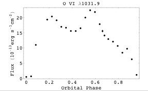
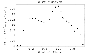
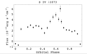
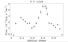
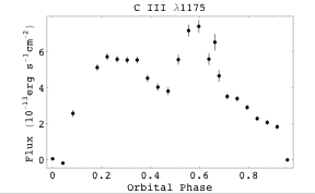
Figure 4: Light curves of prominent lines in the FUSE spectrum of Hercules X-1. A model of the continuum flux has been subtracted. Errors at the $1\sigma$ level are shown. Emission lines shown: (a) S vi$\lambda 933.4$, (b) S vi$\lambda 944.5$, (c) C iii$\lambda 977$, (d) N iii$\lambda 991$, (e) O vi$\lambda 1031.9$, (f) O vi$\lambda 1037.6$, (g) S iv$\lambda 1073$, (h) P v$\lambda 1128$, (i) C iii$\lambda 1176$

In Figure 4 a through i respectively, we show the photometric variation with orbital phase of the emission lines S vi$\lambda 933.4$, S vi$\lambda 944.5$, C iii$\lambda 977$, N iii$\lambda 991$, O vi$\lambda 1031.9$, O vi$\lambda 1037.6$, S iv$\lambda 1073$, P v$\lambda 1128$, and C iii$\lambda 1176$. We have subtracted the background flux using a model that we present in §5. For the N iii line, we remove the flux of nearby airglow lines.

In Table 3, we show the cross-correlation coefficients between the measured lightcurves of the spectral lines and the lightcurves of the disk and star contributions to the continuum lightcurve, as determined by our continuum model.

5 UV Continuum Fits

The UV continuum varies, as the optical continuum does, with the 1.7 day orbital period. The continuum generally peaks near $\phi=0.5$, when the X-ray heated face of the Roche lobe points towards the viewer, but a portion of the normal star may be blocked by the accretion disk, and depending on long-term phase, the actual peak may occur within $\phi\pm\Delta\phi\approx 0.5\pm 0.1$.

The optical/UV orbital light curves do not repeat exactly over the 35-day disk precession cycle. The disk may block X-rays from heating portions of the star, and as it precesses it projects varying areas into the line of sight. The precessing disk should have different eclipse light curves throughout the 35 day cycle.

To fit the UV continuum observed with FUSE, we assume that X-ray heating of HZ Her and the accretion disk cause the entirety of continuum emission. The details of our simulation are similar to those of Vrtilek et al. (1990, especially the appendix), and Howarth & Wilson (1983a) (which was an elaboration on an earlier analysis of Gerend & Boynton, 1976), and binary simulation codes by Wilson & Devinney (1971). The method is summarized in Appendix A.

We fit the spectrum using a reddening $E(B-V)=0.018$ and for the extinction curve, we use Equation 5 in Cardelli, Clayton, & Mathis (1989).

We also use a more modern determination of the distance to Her X-1 (Reynolds et al. 1997). This greater distance requires a larger $\dot{M}$ to reach the same continuum flux. Thus the scale of our $\dot{M}$ values are large compared with those reported earlier from IUE and HST observations. The IUE observations found a range of $-\log\dot{M}=8.30$ to $8.68$ (given changes in the long-term phase during an anomalous low state), whereas the HST found $-\log\dot{M}=8.19\pm 0.06$.

When fit our continuum model to the observed FUSE spectrum from each FUSE observation, we find a range of $-\log\dot{M}=8.12$ to 8.38.

For our fits we ignore wavelength regions that contain prominent emission or absorption lines. We correct for absorption from the first 4 rotational energy levels of interstellar H₂ by multiplying the spectrum by the model presented in §3.

Table 3 gives the best-fit values of the mass accretion rate, $\dot{M}$, which we allow to vary as a free parameter for each FUSE orbit. We also list the reduced $\chi^{2}$.

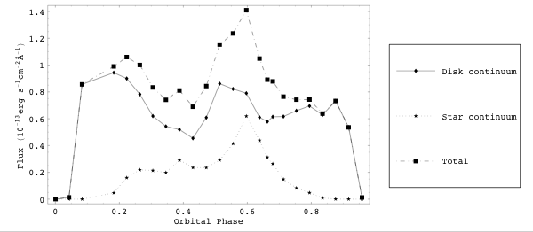
Figure 5: Flux versus orbital phase $\phi$ in our model of the continuum flux in the wavelength range of the O vi doublet. The continuum is separated into disk and stellar components.

We have used our continuum fits to examine the continuum photometry. The model allows us to separate the continuum emission into contributions from the heated face of HZ Her and from the accretion disk. In Figure 5 we show the model flux near the O vi lines split into disk and stellar components.

6 Eclipse Models

We made a simple model for emission from a symmetric precessing accretion disk undergoing eclipse by the Roche lobe of its companion. We then allowed free parameters of that model to vary in order to fit the observed O vi profiles during eclipse ingress and egress.

The disk and Roche lobe geometry are based on the model of Howarth & Wilson (1983a), while the formation of the emission lines follows the model of Horne (1995), and is described in Appendix B. We allow as free parameters the exponent of a radial power law of optical depth and elements of the Mach turbulence matrix. We allow the normalization of the line flux at each orbital phase to vary as a free parameter.

We calculate the eclipsing edge of the Roche lobe of HZ Her assuming corotation with the orbit.

Before fitting the model to the data, we subtracted the mid-eclipse spectrum from all spectra. The origin of the UV mid-eclipse spectra was explored by Anderson et al. (1994) who concluded that it probably does not arise in the accretion disk. The mid-eclipse O vi lines are broad, extending from -200 to $+500$ km s^-1 heliocentric velocity.

We also apply narrow gaussian absorption lines to our model spectra in order to simulate a possible C ii interstellar line near 1036Å, a possible C ii$*$ line near 1037Å, and a O i line near 1039Å. We also include narrow interstellar absorption near the rest wavelengths of the O vi doublet. A narrow absorption line can be seen near the blue component of the doublet at $\lambda=1031.9$Å, but the weaker line at 1037.6Å cannot be seen explicitly. We fix the wavelengths, widths, and optical depths of these lines and do not let them vary in our fit.

We fix all the parameters describing the disk and orbit to those given in Howarth & Wilson (1983a), except the outer radius we fix to $2\times 10^{11}$ cm, following Cheng et al. (1995).

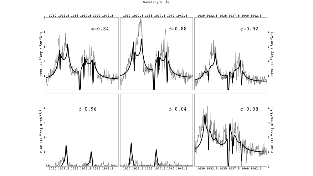
Figure 6: Fits to the O vi lines at phases when the accretion disk is partially eclipsed.

The results are shown in Figure 6.

The reduced $\chi^{2}$ of the fit was 2.8 with 1418 degrees of freedom.

The power law index for the radial dependence on optical depth was $\alpha=-1.2$, between the $\alpha=-1.5$ result found for the N v doublet by similar methods in Boroson et al. (2000) and the $\approx-0.55$ value expected from the simulations of Raymond (1993).

Although we based our fits on the model of Horne (1995) which allows for anisotropic turbulence, the fits do not unambiguously settle on particular values of the Mach matrix. Here, for simplicity, we present a model with isotropic Mach=1 turbulence.

As with the resonance doublets in the near UV, the observed blue component of O vi near eclipse is stronger than the red component, which suggests that much of the line flux is formed where $\tau_{0}\mathrel{<\kern-10.00002pt\lower 3.87495pt\hbox{$\sim$}}1$. However, the doublet ratio is uncertain because strong interstellar C ii and O i absorption lines affect only the red O vi doublet component. Weaker interstellar lines, which we have not modeled, may be present as well, and may preferentially absorb one or the other O vi component.

The model lines are double-peaked outside of eclipse, but one peak of the red component is absorbed by interstellar O i absorption. The observed line profiles are double-peaked at $\phi=0.84$ and double-peaked but broader at $\phi=0.80$. Observations at $\phi=0.35$ and $\phi=0.39$, when narrow line emission predominates, show a dip in the flux at the position of the gap between peaks from the accretion disk line.

The line normalizations we found from our disk eclipse model can be compared with the mass accretion rates inferred from our continuum fits. They do not appear correlated. At some of the phases investigated, we observe only a small fraction of the accretion disk, and none of the illuminated star, so that systematic errors in the line or continuum models may make accurate estimates of $\dot{M}$ impossible. In particular, we have considered the disk flat when it is probably warped, we have not calculated the ionization structure of the disk, we have ignored possible emission by the accretion stream, and we have ignored the role of winds in this system.

Chiang (2001) presented models of accretion disk eclipse in Her X-1 that considered a disk wind. These models were motivated by the lack of double-peaked line profiles in any observations of UV resonance lines. Although the current model predicts double-peaked emission lines when the full disk is visible, the S/N is not strong enough to rule out a double-peaked structure. In addition, interstellar absorption lines coincide with three of the four peaks of the O vi doublet.

It is clear that a model of a partially eclipsed accretion disk with parameters considered standard from previous work provides an excellent match to this data set. There appear to be too many ways to improve the current fit to justify singling one out.

6.1 Anomalous emission at $\phi=0.876$

The fit at $\phi=0.876$ is particularly poor and we suggest that a process in addition to the partial eclipse of a Keplerian accretion disk affects the line profile.

Figure 6 shows that even though more of the disk is eclipsed than at $\phi=0.835$, the emission lines at $\phi=0.876$ are actually stronger. There also appears to be an additional absorption component near the rest wavelength of O vi$\lambda 1032$.

The continuum at $\phi=0.876$ has not increased over the continuum at $\phi=0.835$ as much as the line emission has increased. This is consistent with the earlier result that the X-ray illumination from our line and continuum models at other phases were not correlated.

7 Doppler Tomography

The Doppler tomography method, developed by Marsh and Horne (Marsh & Horne, 1988, Marsh 2005) takes as input an emission line which is broadened by line of sight motion. The line must be observed over a good sampling of the binary orbit. In analogy with medical tomography, a successful Doppler tomogram builds a higher-dimensional view of the object from different observational slices.

Analysis of Doppler shifted emission lines is prone to the confusion of different gas sources which have been projected onto the same observed velocity. The tomographic method presents a transform of the same data into features separated not only by projected velocity, but also by orbital variability.

The output tomogram is not a physical image of an accretion disk, but rather an image in “projected velocity space.” A component of the emission that varies sinusoidally in velocity (but remains constant in flux) is placed at a point in velocity space along a circle with a radius equal to the orbital velocity of that emission component. The phase of the sinusoid determines its position along that circle.

The method assumes that all of the variation in a spectral line must be caused by the orbit changing the projection of the motion into the line of sight. (For example, the change in a spectrum must not be caused by a bright spot being obscured by an opaque object.) Even outside of the conditions in which it strictly applies, however, tomographic images can provide a common view of the data and may suggest directions for further analysis.

Technically, a Doppler tomogram is an inversion of

$$f(v,\phi)=\int_{-\infty}^{\infty}\int_{-\infty}^{\infty}I(v_{x},v_{y})g(v-v_{R})d\,v_{x}d\,v_{y}$$ (2)

which gives the flux $F(v,\phi)$ at the projected velocity $v$ and the orbital phase $\phi$ as a summation of the velocity space tomogram $I(v_{x},v_{y})$ with a line broadening function $g(V-V_{R})$ which is usually narrow. This integral is an instance of a Radon transform. The line broadening function for our FUSE spectra is approximately 0.05Åand for tomographic analysis we assume it is a delta function.

The relation between the radial velocity and the two axes of the Doppler tomogram, $v_{x}$ and $v_{y}$ is given by

$$v_{R}=\gamma-v_{x}\cos 2\pi\phi+v_{y}\sin 2\pi\phi$$ (3)

where $\gamma$ is the systemic velocity of the system.

The formation of the spectrum from the tomogram can be thought of as follows. The phase $\phi$ determines a direction in the velocity space plane, and moving along that line, summing the intensity perpendicular to the line, one ideally forms the spectral line. At $\phi=0.25$, one views from the right in our figures, at $\phi=0.5$ one views from the bottom, and at $\phi=0.75$ one views from the left.

In this paper, we determine $I(v_{x},v_{y})$ from $F(v,\phi)$ by means of Fourier-Filtered Back Projection, which inverts Equation 2 through

$$I(v_{x},v_{y})=\int_{0}^{1}\bar{f}(\gamma-v_{x}\cos 2\pi\phi+v_{y}\sin 2\pi\phi,\phi)d\,\phi$$ (4)

where to calculate $\bar{f}(v,\phi)$ from $f(v,\phi)$, one takes its Fourier transform, multiplies by a ramp filter and a Wiener (optimal) filter based on the noise level, and then takes the inverse Fourier transform.

Although it may seem as if this filtering complicates the method of back-projection, a ramp filter (multiplying the Fourier transform by the frequency) is required in order for back projection to produce a rigorous inversion of Equation 2. Otherwise, back projection would only produce a smeared version of the true tomogram.

Unfortunately, using a ramp filter also magnifies pixel to pixel noise. We apply a standard Wiener filter that assumes a signal amid a noise component that is constant with frequency. We find the power spectrum of the line spectra is well fit by several components of the form $P(\omega)=P_{0}\exp(-k\omega)$ (with $k>0$). The contribution of the signal is negligible at high frequencies $\omega$, where the power spectrum is fit well by a constant noise level $n$. The action of the Wiener filter is then to multiply the power spectrum by $P(\omega)/(n+P(\omega)$, which is nearly 1 when the signal dominates the noise and negligible at high frequencies where the spectrum is almost entirely noise. We used the same form of $P(\omega)$ for each line at each orbital phase, and made a visual comparison between the actual power spectrum and the function $P(\omega)$. Because the filter adapts to different noise levels, the amount of smoothing varies from line to line. For the lines with highest S/N, such as O vi$\lambda 1032$, the turnover frequency for the smoothing filter is on the order of 3 pixels, whereas for weaker lines such as S vi$\lambda 944$, the smoothing is on the order of 10 pixels.

We did not apply the popular method of Maximum Entropy regularization, which awards higher probabilities to those tomograms that provide the least information in the sense that they are smoothest.

7.1 Applications of Doppler Tomography

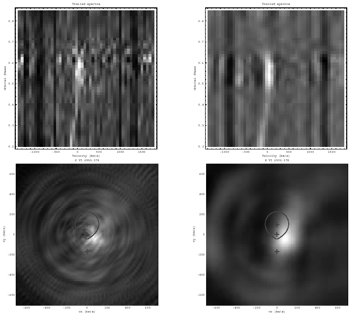
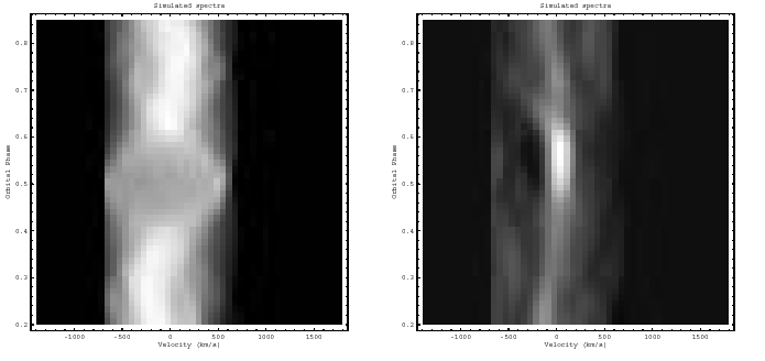
Figure 7: A Fourier-filtered back-projected Doppler tomogram using the FUSE spectra of S vi$\lambda 933$ from $\phi=0.2$ to $\phi=0.85$. The grayscale runs from the minimum to the maximum. Top: the trailed spectrogram (left) and filtered trailed spectrogram (right). Middle: the back-projected tomogram (left) and filtered tomogram (right). Bottom: the trailed spectrogram inverted from the back-projected tomogram (left) and from the filtered tomogram (right).

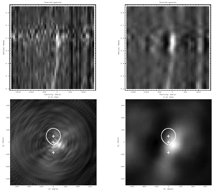
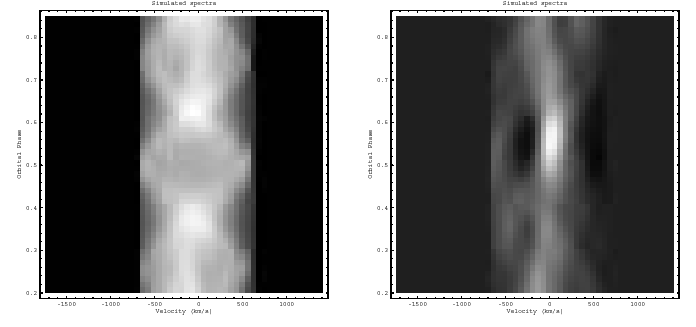
Figure 8: A Fourier-filtered back-projected Doppler tomogram using the FUSE spectra of S vi$\lambda 944$ presented as in Figure 7.

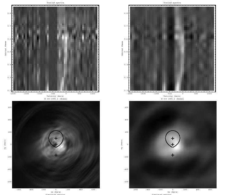
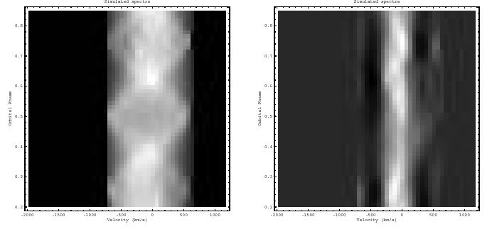
Figure 9: A Fourier-filtered back-projected Doppler tomogram using the FUSE spectra of N iii$\lambda 991.6$ (Bowen process) presented as in Figure 7.

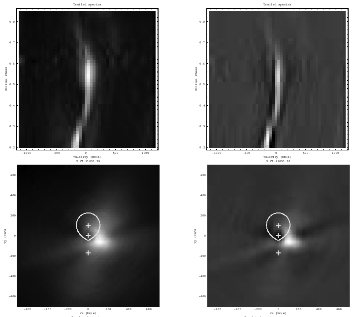
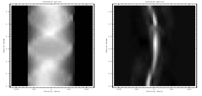
Figure 10: A Fourier-filtered back-projected Doppler tomogram using the FUSE spectra of O vi$\lambda 1031.9$ presented as in Figure 7.

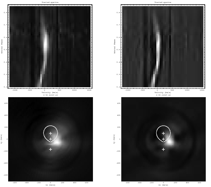
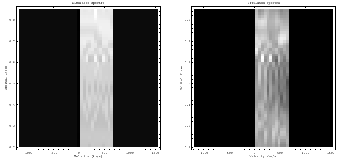
Figure 11: A Fourier-filtered back-projected Doppler tomogram using the FUSE spectra of O vi$\lambda 1037.6$ presented as in Figure 7.

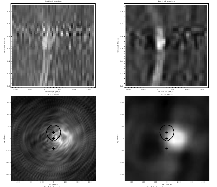
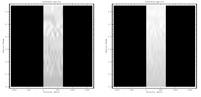
Figure 12: A Fourier-filtered back-projected Doppler tomogram using the FUSE spectra of S iv$\lambda 1073$ presented as in Figure 7.

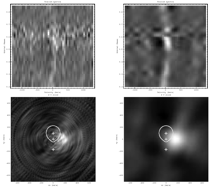
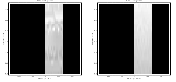
Figure 13: A Fourier-filtered back-projected Doppler tomogram using the FUSE spectra of P v$\lambda 1128$ presented as in Figure 7.

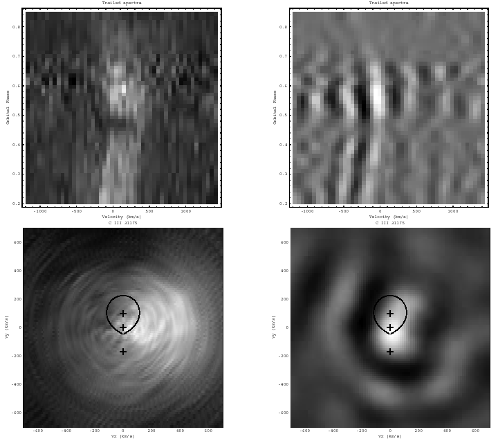
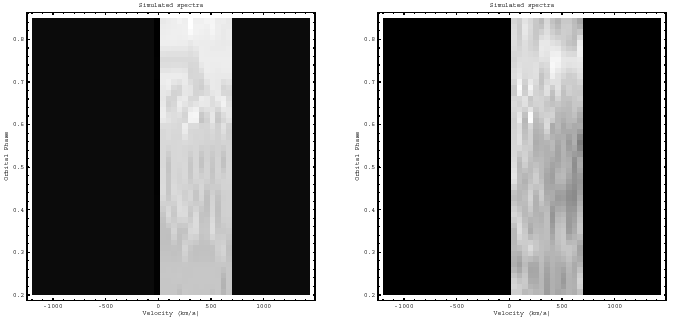
Figure 14: A Fourier-filtered back-projected Doppler tomogram using the FUSE spectra of C iii$\lambda 1176$ presented as in Figure 7.

In Figures 7–14 we show Doppler tomograms of the emission lines of S vi at 933 and 944Å, N iii$\lambda 911$, O vi at 1031Å  and 1037Å, P v$\lambda 1128$, S iv$\lambda 1073$, and C iii$\lambda 1175$. The tomogram of C iii$\lambda 977$ is not shown as it is contaminated by the presence of saturated absorption. We have interpolated between orbital phases for the integration, which we perform between $\phi=0.2$ and $\phi=0.85$. The grayscale of the tomograms extends linearly from the minimum to the maximum.

To understand the C iii multiplet, we consult CHIANTI, a software package and atomic database described in Dere et al. 1997 and Landi et al. 2006. The database, used extensively by stellar and solar astrophysicists, contains energy levels, wavelengths, radiative transition probabilities, and excitation data for many ions. The associated software package, written in IDL (Interactive Data Language), can be used to examine how line ratios vary with temperature and density, subject to certain limiting assumptions. We find that C iii contains emission components at $0,85,168,199,269$, and 367 km s${-1}$ relative to the 1175.59Å component.

We were able to reduce the artifacts by deconvolving with a triple-gaussian $g(V-V_{R})$ in Equation 2. We tried Gaussians of equal weight at velocities $(0,+168,+367)$ km s^-1 (Figure 14) and find there is a single bright spot near the Roche lobe.

A further problem with the C iii multiplet is that the model of the continuum in this region predicts an absorption dip. To reduce artifacts, we use the simpler and smoother Kurucz model atmospheres, with 1Å resolution for all of the tomograms, instead of the models based on actual stellar spectra observed with FUSE, which we have computed with 0.1Å resolution and which include some counting statistics noise.

The signal in the tomograms, except as noted above, is concentrated in a peak offset from the Roche lobe of HZ Her. The traditional signature of an accretion disk is not obviously present. Accretion disks are expected to cause broad line emission that appears as a ring in a tomogram, with diminished flux within the velocity at the edge of the accretion disk, or about 300 km s^-1 for Hercules X-1. If the disk emission is symmetric, we expect it to be centered on the position of the neutron star in velocity space, $(vx,vy)=(0,-169)$.

7.2 Narrow Emission and Broad Absorption Components

There is a simple interpretation of the tomograms in terms of P Cygni lines commonly seen in stellar winds from massive stars (and in HST spectra of Her X-1, Boroson, Kallman, & Vrtilek 2001). P Cygni lines, caused by resonance scattering, are characterized by red-shifted emission and absorption blue-shifted by velocities common in the wind. There is a hint of blue-shifted absorption in the trailed spectrograms at $\phi=0.3-0.6$, although there may be an interstellar absorption line as well at these wavelengths and the gap between the peaks of the accretion disk spectrum could also appear to be absorption.

We note that for many tomograms in addition to the bright spot at $(vx,vy)\approx(150,-30)$, there is a dark spot at $(vx,vy)\approx(-100,50)$. (For O vi$\lambda 1031$, this absorption may have a darker lobe near the rest wavelength from interstellar O vi absorption.) Near the start of the phase range used by our tomograms, at $\phi\approx 0.3$, the observer’s line of sight comes from the lower right in Figure 7. As the line of sight passes through both bright and dark spots, the observer at $\phi\approx 0.3$ sees a diminished central peak in the spectral lines.

At $\phi\approx 0.5-0.6$, the viewer looks at the system from the bottom of the plot, stacking pixels vertically. The result is red-shifted emission (the bright spot) and blue-shifted absorption (the dark spot).

Although the blue-shifted absorption at $\phi=0.3-0.6$ may be explained through the analogy of P Cygni lines, the red-shifted emission at these phases does not fit this explanation. In a P Cygni line, except when a very hot wind is present (as in a Wolf-Rayet star), all the emission is caused by spherically symmetric scattering, so that conservation of photons requires that the forward-scattered flux be nearly equal to the back-scattered (“absorbed”) flux (some portion of the forward-scattered emission is blocked by the star itself). In contrast, any blue-shifted absorption in the Her X-1 spectrum is only a small fraction of the emission. Further, P Cygni emission is only red-shifted because it overlaps with the absorption on the blue end; the actual emission spectrum should be symmetric about zero velocity.

It seems most natural to associate the bright spot with the X-ray heated face of the normal star, as it follows roughly the same light curve and appears near the star and far from the disk on the tomograms. Yet the placement of the spot, or equivalently, the orbital variation with velocity, cannot be accounted for easily by such a model.

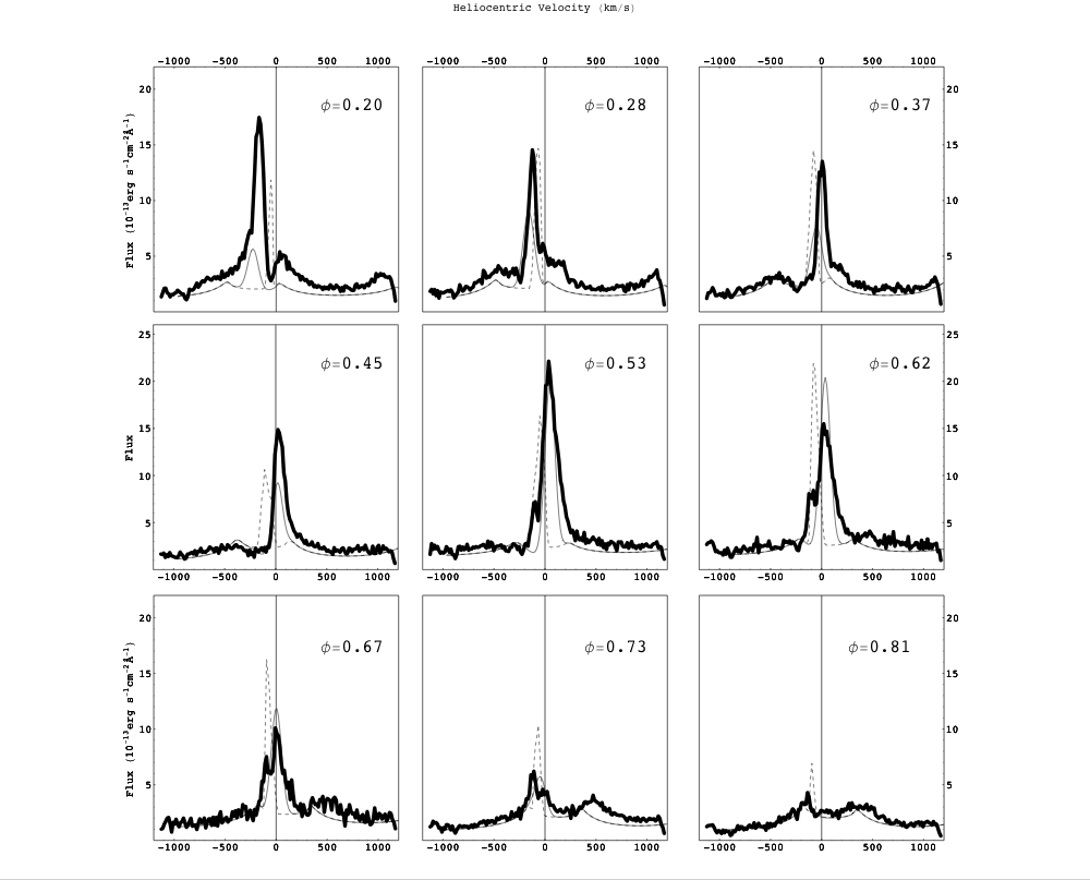
Figure 15: The O vi$\lambda 1032$ emission line averaged over every two FUSE exposures (thick curve), a model of O vi emission on the surface of the noncollapsed star (dashed), and an empirical model of Gaussian emission and absorption models. Both models include flux from a model of the accretion disk.

In Figure 15, we show the observed spectrum near O vi (bold), the spectrum expected if the illuminated surface of HZ Her emits O vi Doppler shifted by the local rotational velocity (dashed), and an empirical Gaussian model of the emission lines. The Doppler shifts predicted from the rotation of the surface of HZ Her are less than observed in the narrow emission lines.

To model the narrow O vi emission lines we adapt our model of the continuum emission. This model takes into account the X-ray shadow cast by the disk and the eclipse of portions of the normal star by the disk. The reprocessed O vi emission is proportional to the incident X-ray flux. We also experimented with a model in which the X-ray illumination was non-isotropic, illuminating HZ Her with greater luminosity at $\phi=0.25$ than at $\phi=0.75$. This model still does not account for the observed velocities.

We also made an empirical model of the lines as Gaussians. The flux in the Gaussian line emission at each phase was proportional to the flux in the stellar component of our continuum model using Kurucz model spectra. The central velocity in this model varies sinusoidally with phase. We added Gaussian absorption to correspond to features seen in HST STIS spectra of the N v$\lambda 1240$, Si iv$\lambda 1400$, and C iv$\lambda 1550$ doublets near $\phi=0.3-0.6$. We set the maximum projected redshift of the emission lines and blueshift of the absorption to occur near $\phi=0.5$, but delayed by $\phi=0.06$, corresponding to a deflection of a wind by the Coriolis effect. The absorption line has maximum covering fraction near $\phi=0.5$ that smoothly varies to 0 at $\phi=0$. (Any wind is probably confined to the cylinder from the star towards the disk, as the emission lines seen in mid-eclipse are only $\sim 1$% of the peak line strength, as observed with the HST FOS by Anderson et al. 1994). Both emission and absorption components have constant width. Both emission and absorption components vary about a central velocity given by the L1 point.

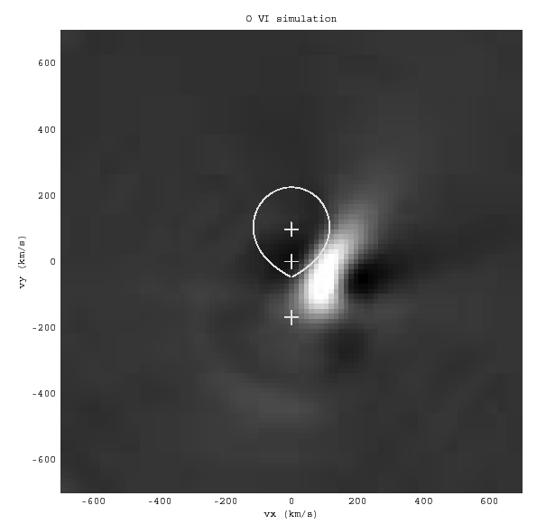
Figure 16: A Doppler tomogram of a simple simulation of the O vi$\lambda 1032$ line as a sum of moving Gaussians and an accretion disk model, with counting statistics included.

When these features are added to the model of the disk spectrum in §6, assumed to move with the neutron star’s 169 km s^-1 orbit, and random counting statistics noise is added, the resulting tomogram (Figure 16) resembles the observed tomogram, while showing only a hint of the presence of an accretion disk. Without the assumed phase delay of $\Delta\phi=0.06$, the bright spot would appear rotated to $vy=0$.

8 Line Ratio Diagnostics

The FUSE spectra show emission lines that may serve as diagnostics of density, temperature, or optical depth.

8.1 C iii line diagnostics

The simultaneous measurement of C iii$\lambda 977$ and C iii$\lambda 1176$ can provide us with an important diagnostic. The C iii 1176/977 ratio is sensitive to density in the range up to about $n_{e}=10^{11}$ cm^-3. At higher densities (up to $n_{e}\sim 10^{15}$), the populations of the ground and metastable levels are entirely determined by collisions. In that regime, the 1176/977 ratio depends only on temperature and the optical depths in the lines.

We ignored flux from the FUSE LiF2B detector near the C iii$\lambda 977$ line, even though this detector recorded flux down to exactly 977Å. The edge of the detector causes the flux measured in this region was significantly lower than the other two detectors, so that including this data would have created an artificial dip at wavelengths $\lambda>977$Å.

The fluxes we measure for C iii$\lambda 977$ are lower limits because of a saturated interstellar absorption line at the rest wavelength. We correct the fluxes for interstellar reddening using E(B-V)=0.018.

We compare the fluxes of the two lines near $\phi=0.6$, when the fluxes peak. If the C iii$\lambda 977$ line behaves similarly to the O vi lines, then the bright narrow emission will, near this phase, have the greatest redshift. If so, the line may be redshifted away from the interstellar absorption and the flux measurement may be more accurate near this phase. If the O vi$\lambda 1032$ line were subject to similar interstellar absorption lines as the C iii$\lambda 977$ line, the flux at $\phi=0.6$ would be diminished by $\sim$20%.

If we measure the raw C iii$\lambda 977$ flux from the two phases surrounding $\phi=0.6$ to be $7\pm 1\times 10^{-13}$ erg s^-1 cm^-2, then we find a 1175/977 ratio of $0.82\pm 0.16$. If we measure the C iii$\lambda 977$ flux at exactly the peak at $\phi=0.6$ and attempt to correct for interstellar absorption lines, we find a ratio of 0.60$\pm 0.09$.

These ratios are at the high end of those predicted by the CHIANTI software, which uses atomic data from the CHIANTI database and computes line ratios, given certain simplifying assumptions (for example, the lines are optically thin and the gas is collisionally ionized and not photoionized). If we consider a density of $n_{e}=10^{13.4}$ cm^-3, the lower ratio found above would restrict the temperature to $T>6\times 10^{4}$ K.

The ratio is rendered uncertain observationally by the saturated interstellar absorption line, and theoretically because of optical depth effects. Raymond (1993) presented models of line emission from an X-ray illuminated accretion disk which took into account optical depth through an escape probability formalism. One version of the model, “COS”, assumed cosmic abundances while the other, “CNO”, assumed that abundances had been altered by CNO processing. The CNO models should be more appropriate for Her X-1. In the two cases the $I(1176)/I(977)$ ratios were 1.3 and 1.1, respectively. The observed emission at $\phi=0.6$ may, however, have an origin not on the disk but on the normal star.

8.2 Bowen fluorescence and N iii$\lambda 991$ emission

The Bowen Fluorescence process (Schachter et al., 1989) arises because of the nearly perfect coincidence of the He ii Ly$\alpha$ and the O iii 2p² – 2p3d resonance line ($\lambda$304), resulting in O iii near–UV primary cascades at $\lambda\lambda$3133, 3444 and secondary cascades at $\lambda$374 back to the ground state. If conditions are right, an additional fluorescence occurs, since the O III$\lambda$374 line is almost coincident with the two N III 2p – 3d resonance lines, resulting in N III optical primary cascades at $\lambda$4634, 4641, 4642. The emission in all of these cascades is completely dominated by the Bowen process; detection of any of them is a clear confirmation. We note that in Her X-1 the process requires substantial optical depth ($\sim 10^{6}$) in the He II Ly$\alpha$ and O III $\lambda$374 pumping lines, because otherwise they will simply escape without conversion to a Bowen line.

In the Sun, Raymond (1978) discovered O III$\lambda$304 Bowen emission. It was found that measurements of O III$\lambda$703, a ground-state Bowen cascade which, therefore, can also be produced by collisional excitation, can serve as a density diagnostic, and compared favorably with other solar estimates of $n_{e}$.

We may use N iii$\lambda$990, an analogous ground–state Bowen cascade produced as a result of the N III primary cascades (“$\lambda$4640”; all other O III and N III ground-state cascades lie below the Lyman limit and hence are unobservable).

The intensity of N iii$\lambda 990$ resulting from Bowen fluorescence is related to the intensity of the Bowen lines at 4640Åby

$$I_{f}(991)=(4640/991)B(\mbox{3p2p})I(4640)$$ (5)

where $B(\mbox{3p2p})$ is the branching ratio of 2p-2s²p² 2D versus 3p-3s. From CHIANTI, we take $B(\mbox{3p2p})=0.55$ and $B(\mbox{3d3p})=0.0058$.

The remainder of the line intensity is therefore from collisional excitation and is given by $I_{c}(991)=I(991)-I_{f}(991)$.

Taking into account the reddening toward Her X-1 implied by E(B-V)=0.018, we find a peak flux in the 991Å line of $8.6\pm 0.7\times 10^{-13}$ erg s^-1 cm^-2. Non-simultaneous measurements of the optical $\lambda$4640 line have a peak flux at similar orbital phases of $7.0\pm 0.2\times 10^{-14}$ erg s^-1 cm^-2 (Still et al. 1997). The optical flux varies from orbit to orbit, and, moreover, probably includes contributions from C iii as well as N iii.

These values imply that 20% of the N iii$\lambda 991$ line flux is the result of the Bowen fluorescence mechanism.

We attempt to relate the density to the Bowen flux by

$$\frac{I_{c}(991)}{I_{f}(991)} = 4$$

$$= \frac{n_{e}N(\mbox{N\,{\sc iii}})q}{B(\mbox{3d3p})B(\mbox{3p2p})N(\mbox{N\,{\sc iii}})\sigma I(374)}$$

$$= 4.9\times 10^{8}n_{e}/I(374)$$

with $N(\mbox{N\,{\sc iii}})$ the density of N iii and $q=6\times 10^{-8}$ s^-1 the excitation rate of the 991Å transition at T=30,000 K.

We estimate an upper bound on the O iii$\lambda 374$ intensity (the line may be optically thick) from the O iii$\lambda 3132$ line observed with the Faint Object Spectrograph on HST by Anderson et al. (1994). We account for the other O iii branches leading to the $\lambda 374$ line by using the observed O iii Bowen spectrum of RR Tel (Selvelli, Danziger, & Bonifacio 2007). We then estimate $I(374)\mathrel{<\kern-10.00002pt\lower 3.87495pt\hbox{$\sim$}}0.032(D/R)^{2}$, with $D=6.6$ kpc the distance to the system and $R$ the radius of the emitting region. Boroson et al. (2000) found $\log n_{e}=13.4\pm 0.2$ for the narrow lines from the ratios of lines observed with HST, and Howarth & Wilson (1983b) found $\log n_{e}=13.3$ from IUE observations. Combining with Equation 8.2, we find $R\mathrel{<\kern-10.00002pt\lower 3.87495pt\hbox{$\sim$}}7\times 10^{10}$ cm.

This is smaller than the size of the accretion disk ($R_{\rm outer}\approx 2\times 10^{11}$ cm). We note that the tomograms show emission from a small region in velocity space.

Another test is provided by a comparison with theoretical models of N iii$\lambda 991$ emission in the absence of the Bowen process. Raymond (1993) found ratios between the N iii line and C iii$\lambda 977$ for the COS model of $I(991)/I(977)=0.34$ and for the CNO model of $I(991)/I(977)=0.53$. The observed ratio of $0.75\pm 0.10$ requires enhancement by Bowen fluorescence and provides an excellent match to the CNO model if only 70% of the N iii$\lambda 991$ line results from collisional excitation.

9 Discussion

The far UV spectrum of Hercules X-1 shows clear evidence for a Keplerian accretion disk. A simple model such a disk can fit the broad O vi emission lines near eclipse. The origin of brighter, narrow emission lines is still unknown. Doppler tomograms place this emission apart from the Roche lobe of HZ Her.

The bright narrow emission component generally follows the flux expected from the illuminated portion of the normal star. However, it appears brighter than expected at $\phi=0.2$ and the velocity excursion is also greater than is accounted for by the rotation of the Roche lobe. A dense portion of a stellar wind that moves along the surface of the star, or that originates at the L1 point and flows back towards the star, would be red-shifted at $\phi=0.5$ and blue-shifted at $\phi=0.25$ and $\phi=0.75$. Although such a model can be made to reproduce the gross features of the line variation, there remain too many possible alternate explanations for this to be convincing. There could be a source of variable emission, absorption, or scattering in addition to the normal star, for example, the gas stream or the surface of the disk.

In the presence of stellar winds, possibly transient or restricted in solid angle, tomography did not show a clear signature of an accretion disk in Hercules X-1.

Although we found that a simple model of an accretion disk generally fit the spectra during eclipse ingress and egress, there was an anomalous observation in which the O vi lines brightened as the disk eclipse progressed. The phase $\phi=0.876$ is in the $\phi=0.8-0.9$ range in which historically “pre-eclipse dips” of X-rays have been observed, and it is tempting to relate the temporary brightening of the lines to a physical cause or result of the dips.

Alternately, an anomalous change to the emission lines could result from a change in shadowing of the X-ray emission. Boroson et al. (2001) concluded that anomalous absorption within the N v$\lambda\lambda 1238,1242$ doublet changed too rapidly to result from material passing over the line of sight. The absorption changed so rapidly probably because of a rapid change in the shadowing of the X-rays which ionize the gas.

Future X-ray spectroscopy missions such as Constellation X may be able to resolve lines from more highly ionized species than the UV and Far UV resonance lines (Vrtilek et al. 2004). If more highly ionized species track disk material better and are not as prevalent in the narrow line region, we may be able to make reliable tomograms of the disk in this or similar systems. Hydrodynamic models of this system may be required to cut down on the vast parameter space of possible gas flows responsible for the spectral signatures observed here.

Appendix A Details of the Model of the Her X-1 Continuum

With one free parameter, the mass accretion rate $\dot{M}$, we model the continuum emission from the accretion disk and X-ray illuminated face of the normal star. We do this not by means of radiative transfer calculations, but by calculating the heated temperatures of both surfaces, and co-adding spectra appropriate for those temperatures, either blackbody spectra, models of stellar spectra, or actual spectra of hot stars observed with FUSE.

Our model of the far UV continuum emission of Her X-1 follows closely the methods of Vrtilek et al. (1990) and Cheng, Vrtilek, & Raymond (1995). We describe the method here in detail, including the minor departures we have made to extend the spectral simulation to the far UV.

The model of the accretion disk temperature as a function of radius, $T(r)$, includes the effects of both internal heating due to viscous forces and heating from X-rays from the neutron star.

When we calculate the disk temperature as a function of radius, $T(r)$, we include both the heat from viscous forces and X-rays from the neutron star. The local energy generated by accretion is given by

$$\sigma T_{0}(r)^{4}=\frac{3GM\dot{M}}{8\pi r^{3}}\left(1-\sqrt{\frac{R}{r}}\right)$$ (A1)

for Stefan-Boltzmann constant $\sigma$, neutron star mass $M$ and radius $R$, and disk mass accretion rate $\dot{M}$ (Shakura & Sunyaev 1973).

For local energy balance, the energy emitted must equal the energy generated plus the X-ray energy absorbed:

$$\sigma T_{\rm eff}^{4}(r)=\sigma T_{0}(r)+\frac{aL_{x}}{4\pi r}\frac{\partial(h/r)}{\partial r}$$ (A2)

where we choose the albedo $a=0.5$, and the disk height at radius $r$ is $h(r)$. The X-ray luminosity is related to the gravitational potential released by accreting matter:

$$L_{\rm x}=0.5\frac{GM\dot{M}}{R}$$ (A3)

These equations, together with vertical hydrostatic equilibrium, can be solved numerically to determine $T(r)$. The surface of the noncollapsed star is also assumed to have an albedo $a=0.5$.

At each small region in the accretion disk, the temperature $T(r)$ is compared with the critical disk temperature, $T_{dc}$. If $T(r)>T_{dc}$, then we assume that the disk region radiates like a blackbody. If $T(r)<T_{dc}$, then we interpolate through our library of actual stellar spectra to find a spectrum appropriate for temperature $T(r)$. From experience fitting HST FOS spectra and fitting the Balmer jump, we fix $T_{dc}=10000$ K so that in practice the disk almost always has blackbody spectra, except at its edge where it is not illuminated by X-rays.

The stellar library from 1150 to 7500Å is described in Cannizzo & Kenyon (1987). The near UV spectra were obtained with IUE and are described in Wu et al. (1982). All the spectra are normalized to have constant flux in the V bandpass and are then scaled to their absolute magnitudes using their V-R colors and the Barnes-Evans relation (Barnes, Evans, & Moffett 1978).

For this paper, we have extended the library of stellar spectra further into the UV by using FUSE spectra of main sequence stars between O 9.5 and A 7. These observations are described briefly in Table 5. Stars of temperature greater than $T_{\rm sc}=18,900$ K are not used in the fits to Her X-1 and are not included in the table. We have interpolated over those wavelengths we expect are affected by interstellar atomic or molecular absorption, and we have applied a filter designed to smooth interstellar lines while retaining stellar features. We de-reddened each spectrum and scaled the flux according to the star’s visual magnitude V. We have tested the method and the use of these stellar spectra by using model stellar spectra as predicted by Kurucz (1979). Plots of far UV spectra in our library, normalized to have a constant V magnitude, are shown in Figure 17.

For the purpose of computing the disk shadow, the disk is assumed to have a fixed opening angle and a fixed tilt from the orbital inclination, although the direction of the disk normal precesses with the X-ray cycle in a manner described by Gerend & Boynton (1976) and Howarth & Wilson (1983a). Because of the finite disk opening angle, the outer regions of the disk can occult the inner regions, and the disk edge itself can radiate, although it is not illuminated by the central X-rays.

The noncollapsed star is assumed to fill its Roche lobe, and its shape, visibility, and illumination by the X-ray source are treated according to methods evolved from Wilson & Devinney (1971) to Howarth & Wilson (1983a). Following those references, we model the eclipse of the disk using the Roche potential. We take into account both limb darkening and the gravity-darkening appropriate for a late-type star. If the temperature of some region on the surface of the star, after X-ray illumination, is greater than some critical temperature $T_{sc}$, we assume the region emits as a blackbody. If the local temperature is less than $T_{sc}$, we again interpolate through our stellar library to find the appropriate stellar spectrum with which the spot radiates. From earlier experience fitting Her X-1 UV spectra, we fix $T_{sc}=18900$ (Cheng, Vrtilek, & Raymond 1995).

The model, as currently realized, does not account for emission or shadowing by a gas stream between the noncollapsed star and disk.

Appendix B Details of the Model of the Disk Lines in Eclipse

Accretion disks in theory have emission lines with a double-peaked shape, with peaks separated by a velocity given approximately by the projection into the line of sight of the orbital velocity at the edge of the accretion disk. For Hercules X-1, with typical neutron star mass, an nearly edge-on inclination, and an outer disk radius of $R\approx 2\times 10^{11}$ cm, we expect the peaks to occur at $\pm 300$ km s^-1. While greater velocities are found within the outer disk radius, each ring at a fixed radius emits down to a Doppler velocity of 0 where the gas moves tangential to the line of sight. Regions of high Doppler velocity arise from progressively smaller regions in the disk, and contribute less to the overall line shape.

We have calculated detailed models of emission from an accretion disk and have fit these to the profiles observed in Her X-1 during eclipse ingress and egress. In reality, the disk is likely to be warped, and in future work we will test individual models of this warped shape. The importance of the demonstration in this paper is that it shows how easy it is to get general agreement with the observed line profiles given the standard picture of the accretion disk.

The method in detail follows that of Horne (1995), which allows for nonisotropic turbulence and for Keplerian shear, that is, the local dispersion in disk velocity as a result of the Keplerian flow itself. This introduces free parameters for the “Mach matrix” describing the turbulent flow, in addition to the power law exponent that we use to as a phenomenological description the strength of the emission line as a function of radius in the disk. For simplicity, we keep the elements of the Mach matrix constant with radius in the disk.

Following Horne (1995), the local line profile is given by

$$I_{\nu}\propto(1-e^{-\tau_{\nu}})$$ (B1)

where the optical depth $\tau_{\nu}$ at frequency $\nu$ is given by

$$\tau_{\nu}=\tau_{0}e^{(V-V_{0})^{2}/2\Delta V^{2}}$$ (B2)

for a given line center optical depth $\tau_{0}$.

The nonisotropic turbulence and shear enter through $\Delta V$, given by

$$\Delta V^{2}=\Delta V^{2}_{\rm therm}+\Delta V^{2}_{\rm shear}+\Delta V^{2}_{\rm turb}$$ (B3)

or

$$\Delta V^{2}/C^{2}_{s} = \frac{\mu}{\gamma A}+(Q\sin i\tan i\sin 2\theta)^{2}+\sin^{2}i(M_{RR}\cos^{2}\theta-2M_{R\theta}\cos\theta\sin\theta$$

$$+ M_{\theta\theta}\sin^{2}\theta)+2\sin i\cos i(M_{ZR}\cos\theta-M_{Z\theta}\sin\theta)+\cos^{2}iM_{ZZ}$$

where $i$ is the orbital inclination, $\mu$ is the mean molecular weight, $\gamma=5/3$, and $A$ is the atomic weight. The shear parameter $Q$ is given by

$$Q=\frac{3}{4}\frac{H}{R}\frac{V_{\rm Kep}}{C_{s}}\frac{\Delta Z}{2H}$$ (B6)

and, for simplicity, is set to $3/4$, the maximum value for an optically thin accretion disk.

The Mach matrix is given by the correlations between components of turbulence in different cylindrical coordinates:

$$M_{ij}\equiv\frac{\langle\delta V_{i}\delta V_{j}\rangle}{C_{s}^{2}}$$ (B7)

where $C_{s}$ is the sound speed.

Symbol	Adopted value	Meaning	Reference
$q$	0.58	Binary mass ratio	Howarth & Wilson 1983a
$M_{\rm ns}$	1.4	Mass of neutron star (M⊙)
$R_{\rm inner}$	106	Inner radius of accretion disk (cm)	Cheng, Vrtilek, & Raymond 1995
$R_{\rm outer}$	2$\times 10^{11}$	Outer radius of accretion disk (cm)	CVR
$a$	0.5	Albedo	CVR
$D$	6600	Distance to system (pc)	Reynolds et al. 1997
EB-V	0.018	Reddening parameter	Boroson et al. 2001
T∗	8100	Polar temperature of normal star (K)	CVR
$\Delta\Psi$	$0.8105$	Disk precession phase offset	H&W
$\theta_{\rm d}$	4.87	Disk thickness (degrees)	H&W
$\alpha_{\rm d}$	28.72	Disk tilt from orbital plane (degrees)	H&W
$a_{*}$	6.35$\times 10^{11}$	Orbital separation, centers of mass (cm)	H&W
$i$	81.25	Orbital inclination (degrees)	H&W

Table 1: Parameters describing the X-ray binary Hercules X-1

Root name	MJD (start)	MJD (end)	Orbital Phase	Exptime (s)	Comments
B0080101001	52069.32464	52069.36421	0.182562	3418
B0080101002	52069.39311	52069.43359	0.223105	3498
B0080101003	52069.46245	52069.50297	0.263900	3501
B0080101004	52069.53186	52069.57233	0.304712	3497
B0080101005	52069.60135	52069.64170	0.345547	3455	Dip in O vi (double-peak gap?)
B0080101006	52069.67566	52069.71106	0.387799	2800	Dip in O vi
B0080101007	52069.74947	52069.78043	0.429904	2675
B0080101008	52069.82233	52069.84980	0.471734	2374
B0080101009	52069.89492	52069.91917	0.513482	2095
B0080101010	52069.96775	52069.98854	0.555305	1796
B0080101011	52070.04000	52070.05792	0.596954	1548
B0080101012	52070.11058	52070.12730	0.638113	1442
B0080101013	52070.15631	52070.16500	0.662651	644
B0080101014	52070.18235	52070.19666	0.679620	1231
B0080101015	52070.22613	52070.26604	0.712899	3447
B0080101016	52070.29521	52070.33540	0.753612	3472
B0080101017	52070.36448	52070.40475	0.794380	3479	O vi$\lambda 1032$ double-peaked
B0080101018	52070.43388	52070.47413	0.835192	3478	O vi$\lambda 1032$ double-peaked
B0080101019	52070.50334	52070.54349	0.876021	3469	Lines anomalously bright
B0080101020	52070.57267	52070.61286	0.916809	3434
B0080101021	52070.64515	52070.68223	0.958526	3204
B0080101022	52070.71889	52070.75160	0.000611	2811	Mid-Eclipse
B0080101023	52070.79200	52070.82097	0.042515	2503
B0080101024	52070.86463	52070.88778	0.083521	2000

Table 2: A log of the FUSE Her X-1 observations.

Exposure	Orbital Phase	Duration (s)	$\dot{M}$ (Kurucz)	$\chi^{2}$ (Kurucz)	$\dot{M}$ (FUSE)	$\chi_{\nu}^{2}$ (FUSE)
			($-\log_{10}$ M⊙)		($-\log_{10}$ M⊙)
1	0.182	3418	8.04	2.7	8.06	2.7
2	0.223	3498	8.07	2.9	8.10	3.0
3	0.264	3501	8.09	3.1	8.19	3.2
4	0.305	3497	8.16	2.9	8.26	3.0
5	0.346	3486	8.21	2.7	8.32	2.9
6	0.388	3059	8.24	2.5	8.33	2.7
7	0.430	2675	8.29	2.4	8.38	2.8
8	0.472	2374	8.20	2.3	8.30	2.5
9	0.513	2095	8.07	2.6	8.18	2.7
10	0.555	1796	8.08	2.4	8.17	2.7
11	0.597	1548	8.13	2.5	8.21	2.6
12	0.638	1444	8.20	2.2	8.27	2.3
13	0.663	751	8.22	1.2	8.30	1.3
14	0.680	1236	8.19	1.6	8.27	1.6
15	0.713	3448	8.17	2.5	8.27	2.6
16	0.754	3473	8.20	2.5	8.22	2.6
17	0.794	3480	8.18	2.3	8.19	2.3
18	0.835	3478	8.22	2.2	8.22	2.2
19	0.876	3469	8.17	2.2	8.18	2.2
20	0.917	3472	8.29	1.7	8.28	1.7
21	0.958	3204	NA	NA	NA	NA
22	0.001	2826	NA	NA	NA	NA
23	0.042	2503	NA	NA	NA	NA
24	0.084	2000	8.10	1.7	8.12	1.7

Table 3: Fits to the Her X-1 continuum as observed with FUSE. $\dot{M}$ (Kurucz) and $\chi^{2}$ (Kurucz) give the mass accretion rate and goodness of fit parameter for the model fit that uses Kurucz spectra while $\dot{M}$ (FUSE) and $\chi^{2}$ (FUSE) give those parameters for fits using a library of FUSE spectra.

Ion	Wavelength (Å)	$r_{\rm star}$	$r_{\rm disk}$	$r_{\rm continuum}$	Comments
S vi	933.4	0.88	0.38	0.67
S vi	944.5	0.88	0.54	0.85
C iii	977	0.90	0.45	0.76	Affected by strong ISM line
N iii	992	0.80	0.62	0.91	Near strong airglow lines
O vi	1031.9	0.74	0.75	0.95
O vi	1037.6	0.82	0.71	0.98
S iv	1073	0.75	0.63	0.88
P v	1128	0.75	0.58	0.86
C iii	1175	0.82	0.65	0.95

Table 4: Correlation coefficients between the light curves of emission lines and continuum components as separated by our model (§5).

Star	Spectral Type	Teff (K)	FUSE Rootname	E(B-V)	V
HD 146813	B 1.5 V	24000	P1014901	0.02	9.06
HD 74662	B 3 V	18000	A1290201	0.09	8.87
(Interpolated)	B 4 V	16500
HD 92288	B 6 V	14000	Z9012801	0.05	7.9
(HD 21672,HD 92536)	B 8 V	11500	(Z9011401,Z9012901)	(0.09,0.04)	(6.63,6.32)
HD 149630	B 9 V	10800	B0910101	0.04	4.2
(HD 109573,HD 181296)	A 0 V	10000	(B0910401,P2500101)	(0.0,0.01)	(5.78,5.03)
HD 31647	A 1 V	9300	C0380901	0.0	4.989
HD 115892	A 2 V	9050	A0410505	0.0	2.75
HD 43940	A 3 V	8850	C0380101	0.0	5.87
HD 11636	A 5 V	8500	A0410101	0.0	2.64
(Interpolated)	A 6 V	8350
HD 187642	A 7 V	8050	D0990101	0.0	0.77

Table 5: FUSE spectra used to form a library of stellar continua versus effective temperature in the far UV.

Figure 1: The mean Her X-1 far UV spectrum observed with FUSE ($<1180$Å) and the HST STIS ($>1150$Å) near orbital phases when the emission is expected to be dominated by the accretion disk. Prominent emission lines are indicated by dotted vertical lines. We show he average of our continuum models using actual FUSE spectra of hot stars together with blackbodies. The component of the model resulting from the X-ray heated face of the normal star is indicated by a dotted curve.

Figure 2: The mean Her X-1 far UV spectrum observed with FUSE ($<1180$Å) and the HST STIS ($>1150$Å) near orbital phases when the emission is expected to be dominated by the X-ray heated face of the normal star. The spectrum is plotted as in Figure 1. The lines and continuum are brighter at these phases, and the lines are narrower.

Figure 3: A sample of the H₂ absorption lines in the spectrum of Her X-1, and a model (dotted lines) with flat normalization, of absorption from rotational levels $J=0$ through $J=3$.

Figure 17: Sample spectra, with spectral type labelled, in the library of FUSE spectra we use to complement our library of IUE and optical spectra. We use this library in the fitting of the Her X-1 continuum. All stars have their V band flux normalized to the same value.

References

- (1) Abgrall, H., Roueff, E., Launay, F., Roncin, J.Y., & Subtil, J.L. 1993a, A&AS, 101, 273
- (2) Abgrall, H., Roueff, E., Launay, F., Roncin, J.Y., & Subtil, J.L. 1993b, A&AS, 101, 323
- (3) Anderson, S.F., Wachter, S., Margon, B., Downes, R.A., Blair, W.P. Halpern, J.P. 1994, ApJ, 436, 319
- (4) Arons, J. 1973, ApJ, 184, 539
- (5) Barnes, T.G., Evans, D.S., & Moffett, T.J. 1978, MNRAS, 183, 285
- (6) Basko, M.M., Sunyaev, R.A., Hatchett, S., & McCray, R. 1977, ApJ, 215, 276
- (7) Begelman, M.C., McKee, C.F., & Shields, G.A. 1983, ApJ, 271, 70
- (8) Begelman, M.C., & McKee, C.F. 1983, ApJ, 271 89
- (9) Bohlin, R.C. 1975, ApJ, 200, 402
- (10) Boroson, B., Vrtilek, S.D., McCray, R., Kallman, T., & Nagase, F. 1996, ApJ, 473, 1079
- (11) Boroson, B., Blair, W.P., Davidsen, A.R, Vrtilek, S.D., Raymond, J., Long, K.S., McCray, R. 1997, ApJ, 473, 1079
- (12) Boroson, B., Kallman, T.R., & Vrtilek, S.D. 2001, ApJ, 562, 925
- (13) Boroson, B., Kallman, T., Vrtilek, S.D., Raymond, J., Still, M., Bautista, M., & Quaintrell, H. 2000, ApJ, 529, 414
- (14) Cannizzo, J.K., & Kenyon, S.J. 1987, ApJ, 320, 319
- (15) Cardelli, J.A., Clayton, G.C., & Mathis, J.S. 1989, ApJ, 345, 245
- (16) Cheng, F.H., Vrtilek, S.D., & Raymond, J.C. 1995, ApJ, 452, 825
- (17) Chiang, J. 2001, ApJ, 549, 537
- (18) Crosa, L, & Boynton, P.E. 1980, ApJ, 235, 999
- (19) Davidson, K., & Ostriker, J.P. 1973, ApJ, 179, 585
- (20) Deeter, J.E., Boynton, P.E., Miyamoto, S., Kitamoto, S., Nagase, F., & Kawai, N. 1991, ApJ, 383, 324
- (21) Dere, K.P., Landi, E., Mason, H.E., Monsignori Fossi, B.C., Young, P.R. 1997, A&AS, 125, 149
- (22) Feldman, P.D., Sahnow, D.J, Kruk, J.W., Murphy, E.M., Moos, H.W. 2001, JGR, 106, 8119
- (23) Gerend, D. & Boynton, P.E. 1976, ApJ, 209, 562
- (24) Giacconi, R., Gursky, H., Kellog, E., Levinson, R., Schreier, E., & Tananbaum, H. 1973, ApJ, 184, 227
- (25) Gillmon, K., Shull, J.M., Tumlinson, J., & Danforth, C. 2006, ApJ, 636, 891
- (26) Horne, K. 1995, A&A, 297, 273
- (27) Howarth, I.R., & Wilson, R. 1983a, MNRAS, 202, 347
- (28) Howarth, I.R., & Wilson, R. 1983b, MNRAS, 204, 1091
- (29) Jimenez-Garate, M.A., Hailey, C.J., den Herder, J.W., Zane, S., Ramsay, G. 2002, ApJ, 578, 391
- (30) Jimenez-Garate, M.A., Raymond, J.C., Liedahl, D.A., & Hailey, C.J. 2005, ApJ, 625, 931
- (31) Ko, Y.-K., & Kallman, T.R. 1994, ApJ, 431, 273
- (32) Kurucz, R.L. 1979, ApJS, 40, 1
- (33) Landi, E., Del Zanna, G., Young, P.R., Dere, K.P., Mason, H.E., Landini, M. 2006, ApJSS, 162, 261
- (34) London, R., McCray, R., & Auer, L.H. 1981, ApJ, 243, 970
- (35) McCandliss, S.R. 2003, PASP, 115, 651
- (36) Maloney, P.R., & Begelman, M.C. 1997, ApJ, 491, L43
- (37) Marsh, T.R., & Horne, K. 1988, MNRAS, 235, 269
- (38) Meyer, F., & Meyer-Hofmeister, E. 1984, A&A, 104, L35
- (39) Middleditch, J., & Nelson, J. 1976, ApJ, 208, 567
- (40) Moos, H.W., Cash, W.C., Cowie, L.L., Davidsen, A.F., Dupree, A.K., Feldman, P.D., Friedman, S.D., Green, J.C., et al. 2000, ApJ, 538, L1
- (41) Raymond, J.C. 1993, ApJ, 412, 267
- (42) Raymond, J.C. 1978, ApJ, 224, 259
- (43) Reynolds, A.P., Quaintrell, H., Still, M.D., Roche, P., Chakrabarty, D., & Levine, S.E. 1997, MNRAS, 288, 43
- (44) Sahnow, D.J., Moos, H.W., Ake, T.B., Andersen, J., Anderson, B.-G., Andre, M., Artis, D., Berman, A.F., Blair, W.P., Brownsberger, K.R., et al. 2000, ApJ, 538, L7
- (45) Schachter, J., Filippenko, A.V., & Kahn, S.M. 1989, ApJ, 340, 1049
- (46) Scott, D.M., & Leahy, D.A. 1999, ApJ, 510, 974
- (47) Scott, D.M., Leahy, D.A., & Wilson, R.B. 2000, ApJ, 539, 392
- (48) Selvelli, P., Danziger, J., & Bonifacio, P. 2007, A&A, 464, 715
- (49) Shakura, N.I., & Syunyaev, R.A. 1973, A&A, 24, 337
- (50) Still, M.D., Quaintrell, H., Roche, P., & Reynolds, A.P. 1997, MNRAS, 292, 52
- (51) Tananbaum, H., Gursky, H., Kellogg, E.M., Levinson, R., Schreier, E., Giacconi, R. 1972, ApJ, 174, L 143
- (52) Vrtilek, S.D., & Cheng, F.H. 1996, ApJ, 465, 915
- (53) Vrtilek, S.D., Quaintrell, H., Boroson, B., Still, M., Fiedler, H., O’Brien, K., McCray, R. 2001, ApJ, 549, 522
- (54) Vrtilek, S.D., Quaintrell, H., Boroson, B., Shields, M. 2004, AN, 325, 209
- (55) Vrtilek et al. 1990. A&A, 235, 162
- (56) Wijers, R.A.M.J, & Pringle, J.E. 1999, MNRAS 308, 207
- (57) Wilson, R.E. & Devinney, E.J. 1971, ApJ, 166, 605
- (58) Wu, C.-C., Boggess, A., Bohlin, R.C., Holm, A.V., Schiffer III, F.H., & Turnrose, B.E. 1982, UVSC Conference, 25
- (59)