Fractal Conductance Fluctuations of Classical Origin

Abstract

In mesoscopic systems conductance fluctuations are a sensitive probe of electron dynamics and chaotic phenomena. We show that the conductance of a purely classical chaotic system with either fully chaotic or mixed phase space generically exhibits fractal conductance fluctuations unrelated to quantum interference. This might explain the unexpected dependence of the fractal dimension of the conductance curves on the (quantum) phase breaking length observed in experiments on semiconductor quantum dots.

A prominent feature of transport in mesoscopic systems is that the conductance as a function of an external parameter (e.g. a gate voltage or a magnetic field) shows reproducible fluctuations caused by quantum interference C. M. Marcus et. al. (1992). A prediction from semiclassical theory that inspired a number of both theoretical and experimental works in the fields of mesoscopic systems and quantum chaos was that in chaotic systems with a mixed phase space these fluctuations would result in fractal conductance curves R. Ketzmerick (1996); L. Hufnagel, R. Ketzmerick, M. Weiss (2001). Such fractal conductance fluctuations (FCFs) have since been confirmed in gold nanowires and in mesoscopic semiconductor billiards in various experiments H. Hegger et. al. (1996); A. S. Sachrajda et. al. (1998); A. P. Micolich et. al. (1998); Y. Ochiai et. al. (1998); Y. Takagaki (2000). In addition FCFs have more recently been predicted to occur in strongly dynamically localized I. Guarneri, M. Terraneo (2001) and in diffusive systems F. A. Pinheiro, C. H. Lewenkopf (2006). Due to the quantum nature of the FCFs it came as a surprise when recent experiments indicated that decoherence does not destroy the fractal nature of the conductance curve but only changes its fractal dimension A. P. Micolich et. al. (2001, 2002). In the present letter we show, that the conductance of purely classical (i.e. incoherent) low-dimensional Hamiltonian systems very fundamentally exhibits fractal fluctuations, as long as transport is at least partially conducted by chaotic dynamics. Thus mixed phase space systems and fully chaotic systems alike generally show FCFs with a fractal dimension that is determined analytically. We show that it is governed by fundamental properties of chaotic dynamics.

In a disordered mesoscopic conductor – which is smaller than the phase coherence length of the charge carriers but large compared to the average impurity spacing – the transmission is the result of the interference of many different, multiply-scattered and complicated paths through the system. As these paths are typically very long compared to the wave length of the charge carriers, the accumulated phase along a path changes basically randomly when an external parameter such as the energy or the magnetic field is varied. This results in a random interference pattern, i.e. reproducible fluctuations in the conductance of a universal magnitude on the order of $2e{{}^{2}}/h$, the so called universal conductance fluctuations (UCFs). For a review see Y. Imry (2002) or D. K. Ferry, S. M. Goodnick (2005). The role of disorder in providing a distribution of random phases can as well be taken by chaos. Thus ballistic mesoscopic cavities like quantum dots in high mobility two-dimensional electron gases that form chaotic billiards show the same universal fluctuations R. A. Jalabert, H. U. Baranger, A. D. Stone (1990); C. M. Marcus et. al. (1992); H. U. Baranger, R. A. Jalabert, A. D. Stone (1993). If the average of the phase gain accumulated on the different paths traversing the system exists, the conductance curves are smooth on parameter scales that correspond to a change of the average phase gain on the order of and smaller than the wave length of the carriers. In systems with mixed phase space, where chaotic and regular motion coexist, this phase gain, however, is typically algebraically distributed and its average phase gain does not exist (neglecting the finiteness of the coherence length and assuming the semiclassical limit $\hbar_{eff}\rightarrow 0$ ; the role of the finite $\hbar_{eff}$ is discussed in L. Hufnagel, R. Ketzmerick, M. Weiss (2001)). Therefore, as shown in R. Ketzmerick (1996), the conductance curve of such a system fluctuates on all parameter scales and forms a fractal. The fractal dimension $D$ is connected to the exponent $\gamma$ of the algebraic distribution of phase gains by $D=2-\frac{\gamma}{2}.$

Experiments on quantum dots that study the dependence of the conductance fluctuations on several system parameters like size and temperature seem to partly contradict the semiclassical theory of fractal scaling A. P. Micolich et. al. (2001, 2002). Namely it was found that with decreasing coherence length the scaling region over which the fractal was observed did not shrink – as would be expected from the semiclassical arguments –, but that the fractal dimension changed. An implicit assumption of the semiclassical theory is that the classical dynamics remains unchanged as the external parameter is varied and thus only phase changes are relevant. In most experimental setups, however, the classical phase space changes with variation of the control parameter. In this article we show that the classical chaotic dynamics itself already leads to fractal conductance curves! Moreover, from this follows that even on very small parameter scales the fluctuations due to changes in the classical dynamics are important. In general the conductance curve is a superposition of two fractals: one originating in interference which is suppressed by decoherence to reveal the fractal fluctuations reflecting the changes in the classical phase space structure. In addition, we predict that FCFs are not only observable in systems with a mixed phase space but in purely chaotic systems.

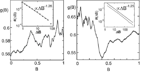
Figure 1: Classical Conductance $g(B)$ through a stadium (left, geometry as in ref. A. S. Sachrajda et. al. (1998)) and square billiard (right, geometry as in ref. A. P. Micolich et. al. (2001)) versus magnetic field $B$. Both fluctuating conductance curves are fractals (see insets and text). Their respective dimensions are $D\approx 1.28$ for the stadium and $D\approx 1.25$ for the square billiard. The fractal dimensions are in good agreement with experimental measurements A. S. Sachrajda et. al. (1998); A. P. Micolich et. al. (2001).

As a starting point of our investigations and to connect it to the experiments we numerically study the classical conductance through a rectangle (hard-wall) and a stadium billiard (soft-wall) as a function of a magnetic field as shown in Fig. 1. (Throughout this article, we will study the transmission, which, in accordance with the Landauer theory of conductance, is proportional to the conductance, see e.g. S. Datta (1995).) Note that not only the phase space of the stadium but also of the rectangle billiard is mixed in the presence of a perpendicular magnetic field. In both cases, a modified version not (a); P. Meakin (1998) of the box-counting analysis clearly reveals the fractal nature of the conductance curves. As the simulation is purely classical, the fractal scaling cannot be caused by interference effects. So what is the underlying mechanism for the fractality of the conductance curve and how can we understand its dimension?

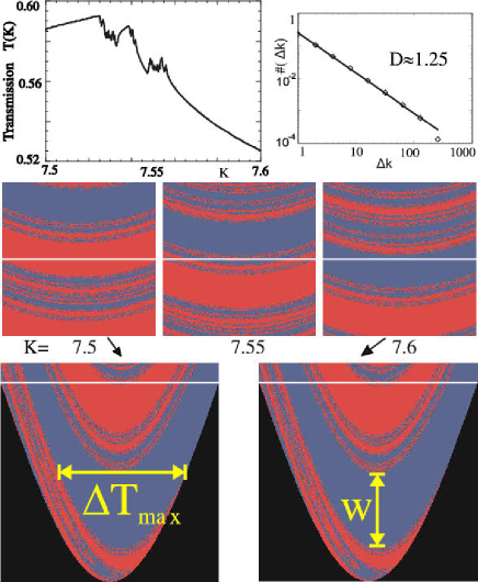
Figure 2: How lobes translate into fluctuations: In the lower row the entryset of the standard map with absorbing boundary conditions at $\pm 3\pi$ for $K=7.5$ and $K=7.6$ resp. can be seen. The three pictures in the center row show the magnification of the central sections of the entryset for three different values of $K=7.5$, $7.55$ and $7.6$. The transmission $T(K)$ for $K=7.5\ldots 7.6$ not (b) is shown in the top left picture. Note that a small change in $K$ shifts the lobes vertically, but conserves the overall phase space structure, and that the largest fluctuations are caused by intersection with the apex of lobes. Starting from $K=7.5$, a large transmission lobe is cut by the horizontal line (see text), i.e. the transmission increases with $K$. In the same way, e.g. the fluctuations of $T(K)$ near $K=7.55$ can be understood. The box-counting analysis reveals a fractal structure (top right).

To study this mechanism in detail we will, because of its numerical and conceptual advantages, analyze the transport in Chirikov’s standard map B. V. Chirikov (1979); S. Fishman, D. R. Grempel, R. E. Prange (1982); A. Altland, M. R. Zirnbauer (1996). This paradigmatic system shows all the richness of Hamiltonian chaos. And since – as will become apparent below – our theory relies only on very fundamental properties of chaotic systems, it is a natural choice as a model system. The standard map is defined by

$$\theta^{\prime} = p+\theta$$

$$p^{\prime} = p+K\sin\theta^{\prime}$$

with momentum $p$ , angle $\theta$ and the ’nonlinearity parameter’ $K$, which drives the dynamics from fully integrable ($K=0$) to fully chaotic ($K\gtrsim 7$). In between the phase space is mixed. The standard map can be seen as the Poincaré surface of a conservative system of two degrees of freedom. As such the map can by viewed to directly correspond to the Poincaré map at the boundary of a chaotic ballistic cavity, connecting it conceptually with the experimental system. We introduce absorbing boundary conditions (see e.g. ref. P. Jacquod, E. V. Sukhorukov (2004)), i.e. when $p$ exceeds (drops below) a maximum (minimum) threshold value, the particle is transmitted (reflected) and leaves the cavity. As can be seen right from the definition of the standard map, the envelope of the entryset (which is, the phase space projection of the injection lead) is simply half a period of a sine function times $K$.

A trajectory entering the system eventually contributes either to the total transmission or reflection, and we mark the corresponding point in the entryset by a color code (transmission: red, reflection: blue). Chaotic dynamics, through its fundamental property of stretching and folding in phase space, leads to a lobe structure (see Fig. 2 (bottom)), which is typical for chaotic systems and not special to the standard map. The distribution of widths $w$ of lobes exhibits a power law

$$n(w)\propto w^{-\alpha}.$$ (1)

The lobe structure is translated into transmission by summing up the intersections of the transmission lobes along a horizontal line, see Fig. 2. A lobe of thickness $w$ gives rise to a maximum contribution $\Delta T\propto w^{\beta}$. Variation of the external parameter $K$ leads to a fractal transmission curve $T(K)$ with $D\approx 1.25$.

How does the fractal dimension depend on the power law distribution of lobe-widths and the curvature of the lobes? To this aim, we study a random sequence of curve segments mimicking the intersection of consecutive lobes of widths $w$, distributed algebraically with exponent $\alpha$ and curved like $w^{\beta}$. We define $X_{i}:=\sum_{j=1}^{i}w_{j}$ and

$$T(X)=(-1)^{i}(X-X_{i})^{\beta}\quad\mbox{:}\quad X_{i}<X\leq X_{i+1}.$$

An example of this curve of “random lobes” with $\alpha=1.9$ and $\beta=\frac{1}{2}$ is shown in Fig. 3 (top). The box-counting analysis clearly reveals a fractal structure.

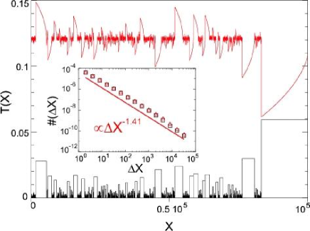
Figure 3: Transmission $T(X)$ for lobes (red upper curve, shifted along the y-axis for clarity) and stripes (black lower curve) for one and the same random distribution with $\alpha=1.9$, $\beta=0.5$. The inset shows the box-counting analysis for the upper (red triangles) and lower transmission curve (black squares). The regression line is drawn for the upper curve, whose fractal dimension is $1.41$.

We further simplify the problem by replacing the lobes by a sequence of stripes of widths $x$ with power law distribution $n(x)\propto x^{\alpha}$. Dispensing with the sign of the fluctuation, the transmission reads

$$T(X)=(X_{i+1}-X_{i})^{\beta}.$$

This yields histogrammatic transmission curves $T(X)$ like the bottom curve of Fig. 3. As shown in the inset, the fractal dimension of the resulting transmission curve remains unchanged compared to the corresponding calculation with random lobes within the precision of the box-counting analysis. Thus, the fractal dimension of the curve does not change noticeably when considering stripes instead of lobes and also when neglecting the sign of each contribution, confirming the intuition, that the fractal dimension depends only on the relative scaling, i.e. $\alpha$ and $\beta$, but not on the detailed form of the curve sections.

For these curves like the bottom one of Fig. 3 with $\alpha-\beta>1$, we can give an analytical expression for the fractal dimension and then estimate the fractal dimension of the transmission curve in the standard map. We apply the box-counting method, which we therefore review shortly (see e.g. P. Meakin (1998) for a more detailed introduction). In this approach the fractal curve lying in a $n-$dimensional space is covered by a $n-$dimensional grid. Let the grid consist of boxes of length scale $s$. The box-counting dimension is then given by

$$D=-\lim_{s\to 0}\frac{\log N(s)}{log(s)},$$ (2)

where $N(s)$ is the number of non-empty boxes. For our problem, we divide $N(s)$ into three contributions $N(s)=n_{a}+n_{b}+n_{c}$, as schematically drawn in Fig. 4(A). The number $n_{a}$ of vertically placed boxes (see mark (a)) covering contributions from stripes of widths $x>s$, reads

$$n_{a}(s)\propto\frac{1}{s}\int_{s}^{\infty}p(x)x^{\beta}dx\propto s^{-(\alpha-\beta)}.$$ (3)

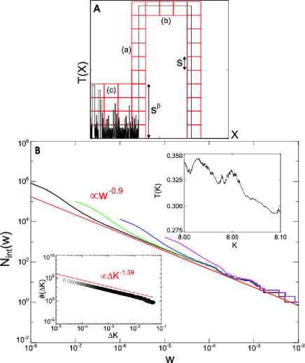
Figure 4: A. Schematic transmission according to Fig. 3 (bottom), covered with boxes of size $s$. There are three contributions marked (a-c). B. Total number $N_{int}(w)=\int_{w}^{\infty}n(w^{\prime})dw^{\prime}$ of lobes (for the open standard map with $|p|<4\pi$) of width larger than $w$ on a double logarithmic scale. The four curves show estimates for increasing resolution $w_{min}=10^{-5}\ldots 10^{-8}$. The curves clearly approach a power law corresponding to $n(w)\propto w^{-1.9}$. The insets show the transmission curve $T(K)$ for values $K=8.0\ldots 8.1$ calculated from $2\times 10^{13}$ trajectories and its box-counting dimension.

Secondly, the number $n_{b}$ of horizontally placed boxes covering horizontal contributions of stripes of widths larger than $s$, see Fig. 4A(b), is given by

$$n_{b}(s)=\frac{1}{s}\int_{s}^{\infty}p(x)xdx<\frac{1}{s}\int_{0}^{\infty}p(x)xdx.$$ (4)

Hence $n_{b}$ scales like $s^{-1}$ and can be neglected in comparison to $n_{a}$ because of $\alpha-\beta>1$. Finally, we determine an upper estimate for the number $n_{c}$ of vertically placed boxes covering the contribution from stripes of widths $x\leq s$. The total length of these widths is $L(s)=\int_{0}^{s}p(x)xdx,$ therefor $L(s)/s$ boxes are needed to cover the length. Inflating all heights of the stripes $x\leq s$ to the maximum possible size $s^{\beta}$, see Fig. 4A(c), we find

$$n_{c}(s)<\frac{L(s)}{s}\,\frac{s^{\beta}}{s}\propto s^{-\alpha+\beta}.$$ (5)

For $s\!\ll\!1$ thus the dominant terms is $n_{a}(s)$. With Eq. (2), $N(s)$ gives rise to the box-counting dimension not (c)

$$D=-\lim_{s\to 0}\frac{\log s^{-\alpha+\beta}}{\log s}=\alpha-\beta.$$ (6)

To connect the analytical result with the calculations of the transmission of the open standard map, we numerically estimate the distribution of lobe-widths in the entryset for $K=8$, finding $\alpha\approx 1.9$, as shown in Fig. 4B. Together with $\beta=\frac{1}{2}$, corresponding to first order Taylor expansion of the cosine function, Eq. (6) predicts a fractal dimension $D\approx 1.4$. Direct analysis of the transmission curve (see insets of Fig. 4B) yields a fractal dimension $D\approx 1.39$, in good agreement with the expected value.

How can a power law distribution of lobe widths emerge in a fully chaotic open system? One might rather expect to find an exponential distribution of lobes in a fully chaotic system. To see why the distribution is algebraic, however, let us examine the simplest case of an open chaotic area preserving map the dynamics of which is governed by a single, positive homogeneous Lyapunov exponent $\lambda$. In each iteration phase space structures are stretched in one direction by $\exp(\lambda)$, shrunk by $\exp(-\lambda)$ in the other and then folded back. The entryset of the open system is thus stretched into lobes of decaying width $w(t_{i})\propto\exp(-\lambda t_{i})$. The phase space volume flux out of the system decays exponentially as it is typical for a fully chaotic phase space, i.e. $\Gamma(t_{i})\propto\exp(-t_{i}/\tau),$ with (mean) dwelltime $\tau$. The area $\Gamma(t_{i})\Delta t$ is the fraction of the exitset that leaves the system at time $t_{i}$. With $t_{i}(w)\propto-\ln(w)/\lambda$ the number of lobes of width $w$ in the exitset is not (d)

$$\#w=\frac{\Gamma(t_{i}(w))\Delta t}{w}\propto\frac{1}{w}\exp(\frac{\ln(w)}{\lambda\tau})=w^{\frac{1}{\lambda\tau}-1}.$$

This suggests that the power law distribution of lobe widths is a generic property even for fully chaotic systems. A quantitative expression for the exponent, however, is not as easy to derive, as e.g. the Lyapunov exponent for the standard map is not homogeneous.

In conclusion, we have shown that transport through chaotic systems due to the typical lobe structure of the phase space in general produces fractal conductance curves, where the fractal dimension reflects the distribution of lobes in the exit- /entryset. In contrast to the semiclassical effect the size of the fluctuations is not universal but depends on specific system parameters. Due to the fractal nature of the classical conductance, however, there is no parameter scale that separates coherent and incoherent fluctuations.

References

- C. M. Marcus et. al. (1992) C. M. Marcus et. al., Phys. Rev. Lett. 69, 506 (1992).
- R. Ketzmerick (1996) R. Ketzmerick, Phys. Rev. B 54, 10841 (1996).
- L. Hufnagel, R. Ketzmerick, M. Weiss (2001) L. Hufnagel, R. Ketzmerick, M. Weiss, Europhys. Lett. 54, 703 (2001).
- H. Hegger et. al. (1996) H. Hegger et. al., Phys. Rev. Lett. 77, 3885 (1996).
- A. S. Sachrajda et. al. (1998) A. S. Sachrajda et. al., Phys. Rev. Lett. 80, 1948 (1998).
- A. P. Micolich et. al. (1998) A. P. Micolich et. al., J. Phys. Condens. Matter 10, 1339 (1998).
- Y. Ochiai et. al. (1998) Y. Ochiai et. al., Semicond. Sci. Technol. 13, A15 (1998).
- Y. Takagaki (2000) Y. Takagaki, Phys. Rev. B 15, 10255 (2000).
- I. Guarneri, M. Terraneo (2001) I. Guarneri, M. Terraneo, Phys. Rev. E 65, 015203 (2001).
- F. A. Pinheiro, C. H. Lewenkopf (2006) F. A. Pinheiro, C. H. Lewenkopf, Brazilian Journal of Physics 36, 379 (2006).
- A. P. Micolich et. al. (2001) A. P. Micolich et. al., Phys. Rev. Lett. 87, 036802 (2001).
- A. P. Micolich et. al. (2002) A. P. Micolich et. al., Physica E 13, 683 (2002).
- Y. Imry (2002) Y. Imry, ed., Introduction to mesoscopic physics (Oxford University Press, 2002).
- D. K. Ferry, S. M. Goodnick (2005) D. K. Ferry, S. M. Goodnick, ed., Transport in nanostructures (Cambridge University Press, 2005).
- R. A. Jalabert, H. U. Baranger, A. D. Stone (1990) R. A. Jalabert, H. U. Baranger, A. D. Stone, Phys. Rev. Lett. 65, 2442 (1990).
- H. U. Baranger, R. A. Jalabert, A. D. Stone (1993) H. U. Baranger, R. A. Jalabert, A. D. Stone, Chaos 3, 665 (1993).
- S. Datta (1995) S. Datta, ed., Electronic Transport in Mesoscopic Systems (Cambridge University Press, 1995).
- not (a) Throughout this article, in order to determine the fractal dimension of a given 2D curve , we used the so called variation method, i.e. we calculated , where for a fractal curve of dimension .
- P. Meakin (1998) P. Meakin, ed., Fractals, scaling and growth far from equilibrium (Cambridge University Press, 1998).
- not (b) The range of the value is close to the first fundamental accelerator mode regime which terminates at . However, trajectories in remaining accelerator mode islands will exit the phase space quickly and do not affect the ensuing statistics.
- B. V. Chirikov (1979) B. V. Chirikov, Phys. Rep. 52, 263 (1979).
- S. Fishman, D. R. Grempel, R. E. Prange (1982) S. Fishman, D. R. Grempel, R. E. Prange, Phys. Rev. Lett. 49, 509 (1982).
- A. Altland, M. R. Zirnbauer (1996) A. Altland, M. R. Zirnbauer, Phys. Rev. Lett. 77, 4536 (1996).
- P. Jacquod, E. V. Sukhorukov (2004) P. Jacquod, E. V. Sukhorukov, Phys. Rev. Lett. 92, 116801 (2004).
- not (c) A numerical calculation of the fractal dimension of transmission curves based on random lobes for various pairs of (,) shows good agreement with the analytical result for .
- not (d) We showed the argument for the exitset and not for the entryset for the sake of clarity. A corresponding relation for the algebraic distribution of lobe widths in the entryset can be derived easily by studying the time-reversed map, that again is a chaotic map with the same properties.