Optimal estimate of probability density functions from experimental data

Abstract

A method providing optimal estimate of probability density functions (PDFs) from time series is proposed. It allows almost arbitrary resolution PDFs when applied to either, sampled analytic functions or digitized data from experiments. When results are compared with PDFs of the same data calculated using the standard histogram method, a remarkable improvement is observed, especially in far lateral regions of the PDF, where low probability events give poor statistics.

Probability density functions (PDFs) are of main interest in physical systems were the statistical description of magnitudes is more appropriate than the detailed behavior in time and/or space of one or more variables. In particular, in research in turbulence, it is of interest to characterize properties with non-Gaussian statistics, especially those related with small scale intermittency Zhou ; Stai , responsible of slowly decaying wings in the PDF of velocity differences at small scales, or the statistics of global magnitudes like pressure Fau or the injected power in confined turbulent flows Lab1 ; Lab2 —characterized by non-symmetric PDFs showing an exponential or stretched exponential wing on the left side. Being the events that contribute to these particular features of the PDF rare, it is not often possible to obtain a good statistics to accurately describe them, and their effect on the the signals could appear to be rather marginal. However, in view of their strength, they are detectable as a non gaussian behavior in the tails of the PDF of the variable under study, and given their importance in the description and understanding of intermittency, among other effects, it is desirable to have a reliable method to estimate the PDF of functions having this kind of features. Additionally, when the PDF of short bursts in a signal is being studied, it is worth to have a tool to estimate it over relatively short time intervals. In these cases, the usual method of building a histogram of the data is inadequate because the number of points available could be not large enough. In this note I propose a simple method to estimate the PDF of a sampled function, like the data obtained when measuring the time evolution of some quantity in an experiment, which produces remarkably good results.

The idea behind the method is simple: given a bounded time function $f(t)$, $t\in[a,b]\subset\mathbb{R}$, with Fourier transform $\mathcal{F}(\omega)$, a sampled version $f_{n}=f(t_{n})$ of $f(t)$, with $t_{n}=nT$, $n=1,\ldots,N$, and $T$ the time interval between samples, is accordingly with the sampling theorem, a complete representation of the continuous function $f(t)$ provided that: i) the function is band limited and ii) the highest frequency contents in the spectrum of $f(t)$ is bounded by the Nyquist frequency, defined as one half of the sampling frequency, i.e.

$$\mathcal{F}(\omega)=0,\qquad|w|>\pi/T.$$ (1)

Thus, although the set of values $\{f_{n}\}$ is nothing but a “small” subset (one having zero-measure) of the set $\{f(t)|t\in[a,b]\subset\mathbb{R}\}$, the Nyquist-Shannon-Kotelnikov sampling theorem allows us to recover all the information contained in the original function from the set of points $\{f_{k}\}$. When $f(t)$ is defined for all $t\in(-\infty,\infty)$, the explicit expression for its reconstructed version, $f_{r}(t)$, in terms of the samples $\{f_{n}\}$ is

$$f_{r}(t)=\sum_{n=-\infty}^{\infty}f_{n}\frac{\sin[\pi(t-nT)/T]}{\pi(t-nT)}.$$ (2)

As we will see later, we do not need $f_{r}(t)$ in the process of building the PDF. If we want to evaluate the PDF in $M$ points $y_{k}$, $k=1,\ldots,M$, a local approximation using few samples near the points $\{(t_{k},f(t_{k}))|f(t_{k})=y_{k},k=1,\ldots,M\}$ will be enough. Now, the usual method of binning the data to make a histogram, which by appropriate normalization gives an estimate of the PDF of $f(t)$, has the obvious drawback that only the values in the set $\{f_{n}\}$ are used. Thus, most of the information to build the PDF of $f(t)$ is lost. Alternatively, if we consider the continuous function $f(t)$, it is intuitively obvious that the probability of finding a certain value $\tilde{y}=f(\tilde{t})$ in the interval $[y,y+\delta y]$ should be proportional to the time $\delta t$ spent by the function in traversing the arbitrarily small neighborhood $[y,y+\delta y]$ of $\tilde{y}$. More precisely, $P(y)\propto|\delta t/\delta y|\longrightarrow 1/|f^{\prime}(t)|$ when $\delta y\longrightarrow 0$. As $f$ can take many times the value $y$ at many different instants $t$, we need to add all these values together over the whole time interval in which the PDF is being calculated. Then, we have

$$P(y)=\frac{1}{N}\sum_{t:y=f(t)}\frac{1}{|f^{\prime}(t)|},$$ (3)

where N is a normalization constant, so that

$$\int_{-\infty}^{\infty}P(y)dy=1.$$ (4)

Equation 3 can be seen as a particular case of equation (5-5) in reference Pap . Note that in (3) the set of values of $y$ can be constructed arbitrarily, provided that $f(t)$ is defined for at least a subset of the values $y$ chosen to evaluate $P(y)$. As a consequence, this allows —as a by-product, to increase arbitrarily the resolution in the evaluation of $P(y)$.

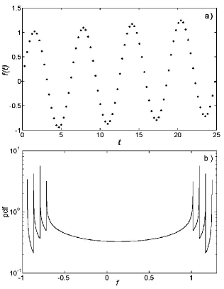
Figure 1: (a) Samples of a function from which the PDF is to be calculated. (b) The resulting PDF, using $5000$ points.

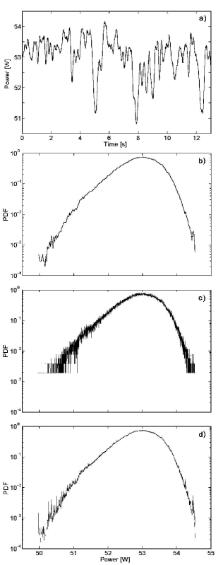
Figure 2: (a) Sample record of power injected in a confined turbulent flow. (b) Its PDF estimate, obtained by binning the data using $200$ bins. (c) A plot showing the result of increasing the number of bins to $4000$. (d) Estimate of the PDF based on equation 3 (see text). The number of points is $4000$, as in the previous plot.

It is important to mention here that a large number of points is not strictly necessary for evaluating a PDF, although this certainly helps in obtaining an accurate evaluation of the normalization constant $N$. The reason is that formula (3) corresponds to the infinitely many points limit of the binning method (the proof is straightforward). What is indeed needed is a good representation of $f(t)$ in the neighborhoods of the zeroes of $f^{\prime}(t)$, where the r.h.s. of equation (3) becomes singular. The advantage of using a rather large number of points $y_{i}$ arises when the normalization constant is calculated: given that $P(y)$ is singular at the roots of $f^{\prime}(t)$, then $N=\int\sum_{t:y=f(t)}|f^{\prime}(t)|^{-1}$ must be evaluated using a low order numerical integration method. In the examples below, the trapezium rule was used, which requires many points to give an accurate result. Another concern is related to the singular values in the r.h.s. of equation (3). One would expect that zeroes in the denominator can appear while running the numerical calculation. This is not the case, because by picking an arbitrary value $y_{k}$, producing a set $\{t_{kj}\}_{j=1,...,m_{k}}$ such that $f(t_{kj})=y_{k}$, getting $f^{\prime}(t_{kj})=0$ for some $j$ is extremely unlike. To date, this has never happened to me, neither in the examples given below nor in other calculations. Thus, to compute a pdf, all we need is a suitable, computationally efficient interpolation scheme to rebuild the function $f$ near $(t,y)$, using some of the samples in the discrete set $\{f_{k}\}$. Although this can be done with the help of equation (2), using an interpolating polynomial through four or six points around the point $(t,f(t))$ is far a better approach, provided that the function corresponding to the samples is smooth enough. When dealing with digitized data, this is ensured by the anti-aliasing filter, except by the remaining electronic noise. I will return to this point later.

To illustrate the method, let us start with the calculation of the PDF of a few cycles of a sinus function plus a “drift”

$$f(t)=\sin(2\pi t/T)+\alpha t,$$ (5)

with suitable values for the parameters, and using a rather poor sampling. From the samples shown in figure 1 (a), and using a third degree interpolating polynomial, the PDF displayed in figure 1 (b) is obtained, using $5000$ point for $P(y)$. Note that the expected singularities in this PDF are remarkably well represented. Of course, there is no way to obtain this result by binning the data shown in figure 1 (a).

As a second example, consider the figure 2 (a), displaying a $13$ s sample of a $3000$ s length record of the power injected to maintain the turbulence in a flow like those in references Lab1 ; Lab2 . As this record was taken specifically to build the PDF of the injected power, some oversampling was performed to allow numerical smoothing on the data. In this case, a cutoff frequency of $50$ Hz was used in the anti-aliasing filter, for a sampling rate of $150$ sps (samples per second). The applied smoothing process is such that the signal spectrum remains unchanged below the filter cutoff frequency. With these two cautionary measures, it is possible to use third order polynomials to locally reconstruct the signal around the points $y_{k}$ chosen to build the PDF, using only four neighboring samples. In figure 2 (b), a PDF built by using the standard binning method is displayed. In this case, $200$ bins were used. The PDF looks very acceptable, thanks to the length of $4.5\times 10^{5}$ samples of the whole data record. If we want to increase the accuracy of the PDF by increasing the number of bins, things begin to go from bad to worse. Figure 2 (c) shows the PDF obtained when $4000$ bins are used. Obviously, trying this is not quite reasonable. However, by using the method that I propose here, a remarkably good $4000$ point estimate of the PDF is effectively obtained, as displayed in figure 2 (d). When compared with figure 2 (a), it is clear that all of the features present there are recovered, but with a highly increased level of detail.

In conclusion, in this note I report a powerful method to estimate the PDF of magnitudes obtained as time series from essentially continuous functions of time, like those resulting by digitizing the signal resulting from the output of an antialiasing filter —a very common experimental scenario. In contrast to the usual binning procedure, the method I propose here can yield, in principle, optimal accuracy and arbitrary resolution in the resulting estimate of the probability density function, even for rather small data sets.

This work benefited of the financial support provided by FONDECYT, under project No. 1040291.

References

- (1) T. Zhou, Z. Hao, L. P. Chua, and S. C. M. Yu, Phys. Rev. E 71, 066307 (2005)
- (2) A. Staicu and W. van de Water, Phys. Rev. Lett. 90, 094501 (2003)
- (3) P. Abry, S. Fauve, P. Flandrin, and C. Laroche, J. Phys. II 4 725 (1994)
- (4) R. Labbé, J.-F. Pinton and S. Fauve, J. Phys. II 6, 1099 (1996)
- (5) J.-F. Pinton, P. C. W. Holdsworth, and R. Labbé, Phys. Rev. E 60, R2452 (1999)
- (6) A. Papoulis, Probability, random variables and stocastic processes, (McGraw-Hill, New York, 1991), chap. 5