Convergence of the
Min-Sum Algorithm for Convex Optimization

Abstract

We establish that the min-sum message-passing algorithm and its asynchronous variants converge for a large class of unconstrained convex optimization problems.

1 Introduction

Consider an optimization problem of the form

(1.1) $$\begin{array}[]{lll}\mathop{\mbox{{\rm minimize}}}\limits&F(x)=&\sum_{C\in{\cal C}}f_{C}(x_{C})\\ \mbox{\rm subject to}&&x\in{\cal X}^{V}.\end{array}$$

Here, the vector of decision variables $x$ is indexed by a finite set $V=\{1,\ldots,n\}$. Each decision variable takes values in the set ${\cal X}$. The set ${\cal C}$ is a collection of subsets of the index set $V$. This collection describes an additive decomposition of the objective function. We associate with each set $C\in{\cal C}$ a component function (or factor) $f_{C}:\ {\cal X}^{C}{\rightarrow}\mathbb{R}$, which takes values as a function of those components $x_{C}$ of the vector $x$ identified by the elements of $C$.

The min-sum algorithm is a method for optimization problems of the form (1.1). It is one of a class of methods know as message-passing algorithms. These algorithms have been the subject of considerable research recently across a number of fields, including communications, artificial intelligence, statistical physics, and theoretical computer science. Interest in message-passing algorithms has been sparked by their success in solving certain classes of NP-hard combinatorial optimization problems, such as the decoding of low-density parity-check codes and turbo codes (e.g., [1, 2, 3]), or the solution of certain classes of satisfiability problems (e.g., [4, 5]).

Despite their successes, message-passing algorithms remain poorly understood. For example, conditions for convergence and accurate resulting solutions are not well characterized.

In this paper, we consider cases where ${\cal X}=\mathbb{R}$, and the optimization problem is continuous. One such case that has been examined previously in the literature is where the objective is pairwise separable (i.e., $|C|\leq 2$, for all $C\in{\cal C}$) and the component functions $\{f_{C}(\cdot)\}$ are quadratic and convex. Here, the min-sum algorithm is known to compute the optimal solution when it converges [6, 7, 8], and sufficient conditions for convergence identify a broad class of problems [9, 10].

Our main contribution is the analysis of cases where the functions are convex but not necessarily quadratic. We establish that the min-sum algorithm and its asynchronous variants converge for a large class of such problems. The main sufficient condition is that of scaled diagonal dominance. This condition is similar to known sufficient conditions for asynchronous convergence of other decentralized optimization algorithms, such as coordinate descent and gradient descent.

Analysis of the convex case has been an open challenge and its resolution advances the state of understanding in the growing literature on message-passing algorithms. Further, it builds a bridge between this emerging research area and the better established fields of convex analysis and optimization.

This paper is organized as follows. The next section studies the min-sum algorithm in the context of pairwise separable convex programs, establishing convergence for a broad class of such problems. Section 3 extends this result to more general separable convex programs, where each factor can be a function of more than two variables. In Section 4, we discuss how our convergence results hold even with a totally asynchronous model of computation. When applied to a continuous optimization problem, messages computed and stored by the min-sum algorithm are functions over continuous domains. Except in very special cases, this is not feasible for digital computers, and in Section 5, we discuss implementable approaches to approximating the behavior of the min-sum algorithm. We close by discussing possible extensions and open issues in Section 6.

2 Pairwise Separable Convex Programs

Consider first the case of pairwise separable programs. These are programs of the form (1.1), where $|C|\leq 2$, for all $C\in{\cal C}$. In this case, we can define an undirected graph $(V,E)$ based on the objective function. This graph has a vertex set $V$ corresponding to the decision variables, and an edge set $E$ defined by the pairwise factors,

$$E=\{C\in{\cal C}:\ |C|=2\}.$$

Definition 1.

(Pairwise Separable Convex Program) A pairwise separable convex program is an optimization problem of the form

(2.1) $$\begin{array}[]{lll}\mathop{\mbox{{\rm minimize}}}\limits&F(x)=&\sum_{i\in V}f_{i}(x_{i})+\sum_{(i,j)\in E}f_{ij}(x_{i},x_{j})\\ \mbox{\rm subject to}&&x\in\mathbb{R}^{V},\end{array}$$

where the factors $\{f_{i}(\cdot)\}$ are strictly convex, coercive, and twice continuously differentiable, the factors $\{f_{ij}(\cdot,\cdot)\}$ are convex and twice continuously differentiable, and

$$M\stackrel{{\scriptstyle\triangle}}{{=}}\min_{i\in V}\ \inf_{x\in\mathbb{R}^{V}}\ \frac{\partial^{2}}{\partial x_{i}^{2}}F(x)>0.$$

Under this definition, the objective function $F(x)$ is strictly convex and coercive. Hence, we can define $x^{*}\in\mathbb{R}^{V}$ to be the unique optimal solution.

2.1 The Min-Sum Algorithm

The min-sum algorithm attempts to minimize the objective function $F(\cdot)$ by an iterative, message-passing procedure. For each vertex $i\in V$, denote the set of neighbors of $i$ in the graph by

$$N(i)=\{j\in V:\ (i,j)\in E\}.$$

Denote the set of edges with direction distinguished by

$$\vec{E}=\{(i,j)\in V\times V:\ i\in N(j)\}.$$

At time $t$, each vertex $i$ keeps track of a “message” from each neighbor $u\in N(i)$. This message takes the form of a function $J^{(t)}_{u\rightarrow i}:\ \mathbb{R}{\rightarrow}\mathbb{R}$. These incoming messages are combined to compute new outgoing messages for each neighbor. The message $J^{(t+1)}_{i\rightarrow j}(\cdot)$ from vertex $i$ to vertex $j\in N(i)$ evolves according to

(2.2) $$J_{i\rightarrow j}^{(t+1)}(x_{j})=\min_{y_{i}}\left(f_{i}(y_{i})+f_{ij}(y_{i},x_{j})+\sum_{u\in N(i)\setminus j}J^{(t)}_{u\rightarrow i}(y_{i})\right)+\kappa^{(t+1)}_{i{\rightarrow}j}.$$

Here, $\kappa^{(t+1)}_{i{\rightarrow}j}$ represents an arbitrary offset term that varies from message to message. Only the relative values of the function $J_{i\rightarrow j}^{(t+1)}(\cdot)$ matter, so the choice of $\kappa^{(t+1)}_{i{\rightarrow}j}$ does not influence relevant information.

At each time $t>0$, a local objective function $b^{(t)}_{i}(\cdot)$ is defined for each variable $x_{i}$ by

(2.3) $$b^{(t)}_{i}(x_{i})=f_{i}(x_{i})+\sum_{u\in N(i)}J^{(t)}_{u{\rightarrow}i}(x_{i}).$$

An estimate $x^{(t)}_{i}$ can be obtained for the optimal value of the variable $x_{i}$ by minimizing the local objective function:

(2.4) $$x^{(t)}_{i}=\mathop{\mbox{{\rm argmin}}}\limits_{y_{i}}b^{(t)}_{i}(y_{i}).$$

The min-sum algorithm requires an initial set of messages $\{J^{(0)}_{i{\rightarrow}j}(\cdot)\}$ at time $t=0$. We make the following assumption regarding these messages:

Assumption 1.

(Min-Sum Initialization) Assume that the initial messages $\{J^{(0)}_{i{\rightarrow}j}(\cdot)\}$ are chosen to be twice continuously differentiable and so that, for each message $J^{(0)}_{i{\rightarrow}j}(\cdot)$, there exists some $z_{i{\rightarrow}j}\in\mathbb{R}$ with

(2.5) $$\frac{d^{2}}{dx_{j}^{2}}J^{(0)}_{i{\rightarrow}j}(x_{j})\geq\frac{\partial^{2}}{\partial x_{j}^{2}}f_{ij}(z_{i{\rightarrow}j},x_{j}),\quad\forall\ x_{j}\in\mathbb{R}.$$

Assumption 1 guarantees that the messages at time $t=0$ are convex functions. Examining the update equation (2.2), it is clear that, by induction, this implies that all future messages are also convex functions. Similarly, since the functions $\{f_{i}(\cdot)\}$ are strictly convex and coercive, and the functions $\{f_{ij}(\cdot,\cdot)\}$ are convex, it follows that the optimization problem in the update equation (2.2) is well-defined and uniquely1 minimized. Finally, each local objective function $b^{(t)}_{i}(\cdot)$ must strictly convex and coercive, and hence each estimate $x^{(t)}_{i}$ is uniquely defined by (2.4).

Assumption 1 also requires that the initial messages be sufficiently convex, in the sense of (2.5). As we will shortly demonstrate, this will be an important condition for our convergence results. For the moment, however, note that it is easy to select a set of initial messages satisfying Assumption 1. For example, one might choose

$$J^{(0)}_{i{\rightarrow}j}(x_{j})=f_{ij}(0,x_{j}).$$

2.2 Convergence

Our goal is to understand conditions under which the min-sum algorithm converges to the optimal solution $x^{*}$, i.e.

$$\lim_{t{\rightarrow}\infty}x^{(t)}=x^{*}.$$

Consider the following diagonal dominance condition:

Definition 2.

(Scaled Diagonal Dominance) An objective function $F:\ \mathbb{R}^{V}{\rightarrow}\mathbb{R}$ is $(\lambda,w)$-scaled diagonally dominant if $\lambda$ is a scalar with $0<\lambda<1$ and $w\in\mathbb{R}^{V}$ is a vector with $w>0$, so that for each $i\in V$ and all $x\in\mathbb{R}^{V}$,

$$\sum_{j\in V\setminus i}w_{j}\left|\frac{\partial^{2}}{\partial x_{i}\partial x_{j}}F(x)\right|\leq\lambda w_{i}\frac{\partial^{2}}{\partial x_{i}^{2}}F(x).$$

Our main convergence result is as follows:

Theorem 1.

Consider a pairwise separable convex program with an objective function that is $(\lambda,w)$-scaled diagonally dominant. Assume that the min-sum algorithm is initialized in accordance with Assumption 1. Define the constant

$$K=\frac{1}{M}\frac{\max_{u}w_{u}}{\min_{u}w_{u}}.$$

Then, the iterates of the min-sum algorithm satisfy

$$\|x^{(t)}-x^{*}\|_{\infty}\leq K\frac{\lambda^{t}}{1-\lambda}\sum_{(u,v)\in\vec{E}}\ \left|\frac{d}{dx_{v}}J^{(0)}_{u{\rightarrow}v}(x^{*}_{v})-\frac{\partial}{\partial x_{v}}f_{uv}(x^{*}_{u},x^{*}_{v})\right|.$$

Hence,

$$\lim_{t{\rightarrow}\infty}x^{(t)}=x^{*}.$$

Proof.

The proof for Theorem 1 will be provided in Section 2.4. ∎

We can compare Theorem 1 to existing results on min-sum convergence in the case of where the objective function $F(\cdot)$ is quadratic. Rusmevichientong and Van Roy [7] developed abstract conditions for convergence, but these conditions are difficult to verify in practical instances. Convergence has also been established in special cases arising in certain applications [11, 12].

More closely related to our current work, Weiss and Freeman [6] established convergence when the factors $\{f_{i}(\cdot),f_{ij}(\cdot,\cdot)\}$ are quadratic, the single-variable factors $\{f_{i}(\cdot)\}$ are strictly convex, and the pairwise factors $\{f_{ij}(\cdot,\cdot)\}$ are convex and diagonally dominated, i.e.

$$\left|\frac{\partial^{2}}{\partial x_{i}\partial x_{j}}f_{ij}(x_{i},x_{j})\right|\leq\frac{\partial^{2}}{\partial x_{i}^{2}}f_{ij}(x_{i},x_{j}),\quad\forall\ (i,j)\in E,\ x_{j},x_{j}\in\mathbb{R}.$$

The results of Malioutov, et al. [10] and our prior work [9] remove the diagonal dominance assumption. However, all of these results are special cases of Theorem 1. In particular, if the a quadratic objective function $F(\cdot)$ decomposes into pairwise factors so that the single-variable factors are quadratic and strictly convex, and the pairwise factors are quadratic convex, then $F(\cdot)$ must be scaled diagonally dominant. This can be established as a consequence of the Perron-Frobenius theorem [10]. Finally, as we will see in Section 3, Theorem 1 also generalizes beyond pairwise decompositions.

2.3 The Computation Tree

In order to prove Theorem 1, we first introduce the notion of the computation tree. This is a useful device in the analysis of message-passing algorithms, originally introduced by Wiberg [13]. Given a vertex $r\in V$ and a time $t$, the computation tree defines an optimization problem that is constructed by “unrolling” all the optimizations involved in the computation of the min-sum estimate $x^{(t)}_{r}$.

Formally, the computation tree is a graph ${\cal T}=({\cal V},{\cal E})$ where each vertex $i\in{\cal V}$ is in labeled by a vertex $\tilde{i}\in V$ in the original graph, through a mapping $\sigma:\ {\cal V}{\rightarrow}V$. This mapping is required to preserve the edge structure of the graph, so that if $(i,j)\in{\cal E}$, then $(\sigma_{i},\sigma_{j})\in E$. Given a vertex $i\in{\cal V}$, we will abuse notation and refer to the corresponding vertex $\sigma_{i}\in V$ in the original graph simply by $i$.

Fixing a vertex $r\in V$ and a time $t$, the computation tree rooted at $r$ and of depth $t$ is defined in an iterative fashion. Initially, the tree consists of a root single vertex corresponding to $r$. At each subsequent step, the leaves in the computation tree are examined. Given a leaf $i$ with a parent $j$, a vertex $u$ and an edge $(u,i)$ are added to the computation tree corresponding to each neighbor of $i$ excluding $j$ in the original graph. This process is repeated for $t$ steps. An example of the resulting graph is illustrated in Figure 1.

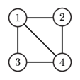
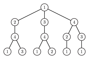
Figure 1: A graph and the corresponding computation tree, rooted at vertex $1$ and of depth $t=3$. The vertices in the computation tree are labeled according to the corresponding vertex in the original graph.

Given the graph ${\cal T}=({\cal V},{\cal E})$, and the correspondence mapping $\sigma$, define a decision variable $x_{i}$ for each vertex $i\in{\cal V}$. Define a pairwise separable objective function $F_{\cal T}:\ \mathbb{R}^{\cal V}{\rightarrow}\mathbb{R}$, by considering factors of the form:

1. For each $i\in{\cal V}$, add a single-variable factor $f_{i}(x_{i})$ by setting $f_{i}(x_{i})\stackrel{{\scriptstyle\triangle}}{{=}}f_{\sigma_{i}}(x_{i})$.

2. For each $(i,j)\in{\cal V}$, add a pairwise factor $f_{ij}(x_{i},x_{j})$ by setting $f_{ij}(x_{i},x_{j})\stackrel{{\scriptstyle\triangle}}{{=}}f_{\sigma_{i}\sigma_{j}}(x_{i},x_{j})$.

3. For each $i\in{\cal V}$ that is a leaf vertex with parent $j$, add a single-variable factor $J^{(0)}_{u{\rightarrow}\sigma_{i}}(x_{i})$, for each neighbor $u\in N(\sigma_{i})\setminus\sigma_{j}$ of $i$ in the original graph, excluding $j$.

Now, let $\tilde{x}$ be the optimal solution to the minimization of the computation tree objective $F_{\cal T}(\cdot)$. By inductively examining the operation of the min-sum algorithm, it is easy to establish that the component $\tilde{x}_{r}$ of this solution at the root of the tree is precisely the min-sum estimate $x^{(t)}_{r}$.

The following lemma establishes that the computation tree inherits the scaled diagonal dominance property from the original objective function.

Lemma 1.

Consider a pairwise separable convex program with an objective function that is $(\lambda,w)$-scaled diagonally dominant. Assume that the min-sum algorithm is initialized in accordance with Assumption 1, and let ${\cal T}=({\cal V},{\cal E})$ be a computation tree associated with this program. Then, the computation tree objective function $F_{\cal T}(\cdot)$ is also ($\lambda,w)$-scaled diagonally dominant.

Proof.

Given a vertex $i\in{\cal V}$, let $N^{\cal V}(i)$ be the neighborhood in the computation tree, and let $N(i)$ be the neighborhood of the corresponding vertex in the original graph. If $i\in{\cal V}$ is an interior vertex of the computation tree, then

$$\begin{split}\@ADDCLASS{ltx_eqn_lefteqn}$\displaystyle\sum_{u\in{\cal V}\setminus i}w_{u}\left|\frac{\partial^{2}}{\partial x_{i}\partial x_{u}}F_{\cal T}(x)\right|$\mbox{}\hfil&\\ &=\sum_{u\in N^{\cal V}(i)}w_{u}\left|\frac{\partial^{2}}{\partial x_{i}\partial x_{u}}f_{iu}(x_{i},x_{u})\right|\\ &\leq\lambda w_{i}\left(\frac{\partial^{2}}{\partial x_{i}^{2}}f_{i}(x_{i})+\sum_{u\in N^{\cal V}(i)}\frac{\partial^{2}}{\partial x_{i}^{2}}f_{iu}(x_{i},x_{u})\right)\\ &=\lambda w_{i}\frac{\partial^{2}}{\partial x_{i}^{2}}F_{\cal T}(x),\end{split}$$

where the inequality follows from the scaled diagonal dominance of the original objective function $F(\cdot)$.

Similarly, if $i$ is a leaf vertex with parent $j$,

$$\begin{split}\@ADDCLASS{ltx_eqn_lefteqn}$\displaystyle\sum_{u\in{\cal V}\setminus i}w_{u}\left|\frac{\partial^{2}}{\partial x_{i}\partial x_{u}}F_{\cal T}(x)\right|$\mbox{}\hfil&\\ &=w_{j}\left|\frac{\partial^{2}}{\partial x_{i}\partial x_{j}}f_{ij}(x_{i},x_{j})\right|\\ &\leq w_{j}\left|\frac{\partial^{2}}{\partial x_{i}\partial x_{j}}f_{ij}(x_{i},x_{j})\right|+\sum_{u\in N(i)\setminus j}w_{u}\left|\frac{\partial^{2}}{\partial x_{i}\partial x_{u}}f_{iu}(x_{i},z_{u{\rightarrow}i})\right|\\ &\leq\lambda w_{i}\left(\frac{\partial^{2}}{\partial x_{i}^{2}}f_{i}(x_{i})+\frac{\partial^{2}}{\partial x_{i}^{2}}f_{ij}(x_{i},x_{j})+\sum_{u\in N(i)\setminus j}\frac{\partial^{2}}{\partial x_{i}^{2}}f_{iu}(x_{i},z_{u{\rightarrow}i})\right)\\ &\leq\lambda w_{i}\left(\frac{\partial^{2}}{\partial x_{i}^{2}}f_{i}(x_{i})+\frac{\partial^{2}}{\partial x_{i}^{2}}f_{ij}(x_{i},x_{j})+\sum_{u\in N(i)\setminus j}\frac{\partial^{2}}{\partial x_{i}^{2}}J^{(0)}_{u{\rightarrow}i}(x_{i})\right)\\ &=\lambda w_{i}\frac{\partial^{2}}{\partial x_{i}^{2}}F_{\cal T}(x).\end{split}$$

Here, the second inequality follows from the scaled diagonal dominance of the original objective function $F(\cdot)$, and the third inequality follows from Assumption 1. ∎

2.4 Proof of Theorem 1

In order to prove Theorem 1, we will study the evolution of the min-sum algorithm under a set of linear perturbations. Consider an arbitrary vector $p\in\mathbb{R}^{\vec{E}}$ with one component $p_{i{\rightarrow}j}$ for each $i\in V$ and $j\in N(i)$. Given an arbitrary vector $p$, define $\{J^{(t)}_{i{\rightarrow}j}(\cdot,p)\}$ to be the set of messages that evolve according to

(2.6) $$\begin{split}J^{(0)}_{i{\rightarrow}j}(x_{j},p)&=J^{(0)}_{i{\rightarrow}j}(x_{j})+p_{i{\rightarrow}j}x_{j},\\ J_{i\rightarrow j}^{(t+1)}(x_{j},p)&=\min_{y_{i}}\left(f_{i}(y_{i})+f_{ij}(y_{i},x_{j})+\sum_{u\in N(i)\setminus j}J^{(t)}_{u\rightarrow i}(y_{i},p)\right)\\ &\quad+\kappa^{(t+1)}_{i{\rightarrow}j}.\end{split}$$

Similarly, define $\{b^{(t)}_{i}(\cdot,p)\}$ and $\{x^{(t)}_{i}(p)\}$ to be the resulting local objective functions and optimal value estimates under this perturbation:

$$b^{(t)}_{i}(x_{i},p) =f_{i}(x_{i})+\sum_{u\in N(i)}J^{(t)}_{u{\rightarrow}i}(x_{i},p),$$

$$x^{(t)}_{i}(p) =\mathop{\mbox{{\rm argmin}}}\limits_{y_{i}}b^{(t)}_{i}(y_{i},p).$$

The following simple lemma gives a particular choice of $p$ for which the min-sun algorithm yields the optimal solution at every time.

Lemma 2.

Define the vector $p^{*}\in\mathbb{R}^{\vec{E}}$ by setting, for each $i\in V$ and $j\in N(i)$,

$$p^{*}_{i{\rightarrow}j}=\frac{\partial}{\partial x_{j}}f_{ij}(x^{*}_{i},x^{*}_{j})-\frac{d}{dx_{j}}J^{(0)}_{i{\rightarrow}j}(x^{*}_{j}).$$

Then, at every time $t\geq 0$,

(2.7) $$\frac{\partial}{\partial x_{j}}J^{(t)}_{i{\rightarrow}j}(x^{*}_{j},p^{*})=\frac{\partial}{\partial x_{j}}f_{ij}(x^{*}_{i},x^{*}_{j}),$$

and $x^{(t)}_{j}(p^{*})=x^{*}_{j}$.

Proof.

Note that the first order optimality conditions for $F(x)$ at $x^{*}$ imply that, for each $j\in V$,

$$\frac{d}{dx_{j}}f_{i}(x^{*}_{j})+\sum_{i\in N(j)}\frac{\partial}{\partial x_{j}}f_{ij}(x^{*}_{i},x^{*}_{j})=0.$$

If (2.7) holds at time $t$, this is exactly the first order optimality condition for the minimization of $b^{(t)}_{j}(\cdot,p^{*})$, thus $x^{(t)}_{j}(p^{*})=x^{*}_{j}$.

Clearly (2.7) holds at time $t=0$. Assume it holds at time $t\geq 0$. Then, when $x_{j}=x^{*}_{j}$, the minimizing value of $y_{i}$ in (2.7) is $x^{*}_{i}$. Hence, (2.7) holds at time $t+1$. ∎

Next, we will bound the sensitivity of the estimate $x^{(t)}_{i}(p)$ to the choice of $p$. The main technique employed here is analysis of the computation tree described in Section 2.3. In particular, the perturbation $p$ impacts the computation tree only through the leaf vertices at depth $t$. The scaled diagonal dominance property of the computation tree, provided by Lemma 1, can then be used to guarantee that this impact is diminishing in $t$.

Lemma 3.

We have, for all $p\in\mathbb{R}^{\vec{E}}$, $r\in V$, $(u,v)\in\vec{E}$, and $t\geq 0$,

$$\left|\frac{\partial}{\partial p_{u{\rightarrow}v}}x^{(t)}_{r}(p)\right|\leq K\frac{\lambda^{t}}{1-\lambda}.$$

Proof.

Fix $r\in V$, and let ${\cal T}=({\cal V},{\cal E})$ be the computation tree rooted at $r$ after $t$ time steps. Let $F_{\cal T}(x,p)$ be the objective value of this computation tree, and let

$$\tilde{x}(p)=\mathop{\mbox{{\rm argmin}}}\limits_{x}F_{\cal T}(x,p),$$

so that

$$\tilde{x}_{r}(p)=x^{(t)}_{r}(p).$$

By the first order optimality conditions, for any $j\in{\cal V}$,

$$\frac{\partial}{\partial x_{j}}F_{\cal T}(\tilde{x}(p),p)=0.$$

If $j$ is an interior vertex of ${\cal T}$, this becomes

(2.8) $$\frac{d}{dx_{j}}f_{j}(\tilde{x}_{j}(p))+\sum_{i\in N(j)}\frac{\partial}{\partial x_{j}}f_{ij}(\tilde{x}_{i}(p),\tilde{x}_{j}(p))=0.$$

If $j$ is a leaf with parent $u$, we have

(2.9) $$\frac{d}{dx_{j}}f_{j}(\tilde{x}_{j}(p))+\frac{\partial}{\partial x_{j}}f_{uj}(\tilde{x}_{u}(p),\tilde{x}_{j}(p))\\ +\sum_{i\in N(j)\setminus u}\left(\frac{\partial}{\partial x_{j}}J^{(0)}_{i{\rightarrow}j}(\tilde{x}_{j}(p))+p_{i{\rightarrow}j}\right)=0.$$

Now, fixed some directed edge $(a,b)$, and differentiate (2.8)–(2.9) with respect to $p_{a{\rightarrow}b}$. We have, for an interior vertex $j$,

$$\begin{split}0&=\frac{d^{2}}{dx_{j}^{2}}f_{j}(\tilde{x}_{j}(p))\frac{\partial}{\partial p_{a{\rightarrow}b}}\tilde{x}_{j}(p)\\ &\quad+\sum_{i\in N(j)}\frac{\partial^{2}}{\partial x_{j}^{2}}f_{ij}(\tilde{x}_{i}(p),\tilde{x}_{j}(p))\frac{\partial}{\partial p_{a{\rightarrow}b}}\tilde{x}_{j}(p)\\ &\quad+\sum_{i\in N(j)}\frac{\partial^{2}}{\partial x_{i}\partial x_{j}}f_{ij}(\tilde{x}_{i}(p),\tilde{x}_{j}(p))\frac{\partial}{\partial p_{a{\rightarrow}b}}\tilde{x}_{i}(p),\end{split}$$

and for a leaf vertex $j$ with parent $u$,

$$\begin{split}0&=\frac{d^{2}}{dx_{j}^{2}}f_{j}(\tilde{x}_{j}(p))\frac{\partial}{\partial p_{a{\rightarrow}b}}\tilde{x}_{j}(p)\\ &\quad+\frac{\partial^{2}}{\partial x_{j}^{2}}f_{uj}(\tilde{x}_{u}(p),\tilde{x}_{j}(p))\frac{\partial}{\partial p_{a{\rightarrow}b}}\tilde{x}_{j}(p)\\ &\quad+\frac{\partial^{2}}{\partial x_{u}\partial x_{j}}f_{uj}(\tilde{x}_{u}(p),\tilde{x}_{j}(p))\frac{\partial}{\partial p_{a{\rightarrow}b}}\tilde{x}_{u}(p)\\ &\quad+\sum_{i\in N(j)\setminus u}\left(\frac{\partial^{2}}{\partial x_{j}^{2}}J^{(0)}_{i{\rightarrow}j}(\tilde{x}_{j}(p))\frac{\partial}{\partial p_{a{\rightarrow}b}}\tilde{x}_{j}(p)+\mathbb{I}_{\left\{(a,b)=(i,j)\right\}}\right).\end{split}$$

We can write this system of equations in matrix form, as

(2.10) $$\Gamma v^{a{\rightarrow}b}+h^{a{\rightarrow}b}=0.$$

Here, $v^{a{\rightarrow}b}\in\mathbb{R}^{\cal V}$ is a vector with components

$$v^{a{\rightarrow}b}_{j}=\frac{\partial}{\partial p_{a{\rightarrow}b}}\tilde{x}_{j}(p).$$

The vector $h^{a{\rightarrow}b}\in\mathbb{R}^{\cal V}$ has components

$$h^{a{\rightarrow}b}_{j}=\mathbb{I}_{\left\{\text{$j$ is a leaf vertex of type $a$ with a parent of type $b$}\right\}}.$$

The symmetric matrix $\Gamma\in\mathbb{R}^{{\cal V}\times{\cal V}}$ has components as follows:

1. If $j$ is an interior vertex,

   $$\Gamma_{jj}=\frac{d^{2}}{dx_{j}^{2}}f_{j}(\tilde{x}_{j}(p))+\sum_{i\in N(j)}\frac{\partial^{2}}{\partial x_{j}^{2}}f_{ij}(\tilde{x}_{i}(p),\tilde{x}_{j}(p)).$$

2. If $j$ is an interior vertex and $i\in N(j)$,

   $$\Gamma_{ij}=\frac{\partial^{2}}{\partial x_{i}\partial x_{j}}f_{ij}(\tilde{x}_{i}(p),\tilde{x}_{j}(p)).$$

3. If $j$ is a leaf vertex with parent $u$,

   $$\begin{split}\Gamma_{jj}&=\frac{d^{2}}{dx_{j}^{2}}f_{j}(\tilde{x}_{j}(p))+\frac{\partial^{2}}{\partial x_{j}^{2}}f_{uj}(\tilde{x}_{u}(p),\tilde{x}_{j}(p))\\ &\quad+\sum_{i\in N(j)\setminus u}\frac{\partial^{2}}{\partial x_{j}^{2}}J^{(0)}_{i{\rightarrow}j}(\tilde{x}_{j}(p)),\\ \Gamma_{uj}&=\frac{\partial^{2}}{\partial x_{u}\partial x_{j}}f_{uj}(\tilde{x}_{u}(p),\tilde{x}_{j}(p)).\end{split}$$

4. All other entries of $\Gamma$ are zero.

Note that $\Gamma=\nabla^{2}_{x}F_{\cal T}(\tilde{x}(p),p)$. Then, Lemma 1 implies that

(2.11) $$\sum_{i\in{\cal V}\setminus j}w_{i}|\Gamma_{ij}|\leq\lambda w_{j}\Gamma_{jj}.$$

Define, for vectors $x\in\mathbb{R}^{\cal V}$, the weighted sup-norm

$$\|x\|^{w}_{\infty}=\max_{j\in{\cal V}}|x_{j}|/w_{j}.$$

For a linear operator $A:\ \mathbb{R}^{\cal V}{\rightarrow}\mathbb{R}^{\cal V}$, The corresponding induced operator norm is given by

$$\|A\|^{w}_{\infty}=\max_{j\in{\cal V}}\frac{1}{w_{j}}\sum_{i\in{\cal V}}w_{i}|A_{ji}|.$$

Define the matrices

$$\begin{split}D&=\mathop{\mbox{{\rm diag}}}(\Gamma),\\ R&=I-D^{-1}\Gamma.\end{split}$$

Then, (2.11) implies that

$$\|R\|^{w}_{\infty}\leq\lambda<1.$$

Hence, the matrix $I-R=D^{-1}\Gamma$ is invertible, and

$$\left(D^{-1}\Gamma\right)^{-1}=(I-R)^{-1}=\sum_{s=0}^{\infty}R^{s}.$$

Examining the linear equation (2.10), we have

$$v^{a{\rightarrow}b}=-\Gamma^{-1}h^{a{\rightarrow}b}=-(I-R)^{-1}D^{-1}h^{a{\rightarrow}b}=-\sum_{s=0}^{\infty}R^{s}D^{-1}h^{a{\rightarrow}b}.$$

We are interested in bounding the value of the component $v^{a{\rightarrow}b}_{r}$ (recall that $v^{a{\rightarrow}b}_{r}=\partial x^{(t)}_{r}(p)/\partial p_{a{\rightarrow}b}$). Hence, we have

$$v^{a{\rightarrow}b}_{r}=-\sum_{s=0}^{\infty}\left[R^{s}D^{-1}h^{a{\rightarrow}b}\right]_{r}.$$

Since $h^{a{\rightarrow}b}$ is zero on interior vertices, and any leaf vertex is distance $t$ from the root $r$, we have

$$\left[R^{s}D^{-1}h^{a{\rightarrow}b}\right]_{r}=0,\quad\forall\ s<t.$$

Thus,

$$v^{a{\rightarrow}b}_{r}=-\sum_{s=t}^{\infty}\left[R^{s}D^{-1}h^{a{\rightarrow}b}\right]_{r}.$$

Then,

$$\begin{split}|v^{a{\rightarrow}b}_{r}|/w_{r}&\leq\left\|\sum_{s=t}^{\infty}R^{s}D^{-1}h^{a{\rightarrow}b}\right\|^{w}_{\infty}\\ &\leq\sum_{s=t}^{\infty}\left\|R^{s}\right\|^{w}_{\infty}\left\|D^{-1}h^{a{\rightarrow}b}\right\|^{w}_{\infty}\\ &\leq\frac{\lambda^{t}}{1-\lambda}\left\|D^{-1}h^{a{\rightarrow}b}\right\|^{w}_{\infty}\\ &\leq\frac{\lambda^{t}}{1-\lambda}\max_{i\in V}\sup_{x\in\mathbb{R}^{V}}\left(w_{i}\frac{\partial^{2}}{\partial x_{i}^{2}}F(x)\right)^{-1}\\ &\leq M\frac{\lambda^{t}}{1-\lambda}\max_{i\in{\cal V}}\frac{1}{w_{i}}.\end{split}$$

∎

The following lemma combines the results from Lemmas 2 and 3. Theorem 1 follows by taking $p=0$.

Lemma 4.

Given an arbitrary vector $p\in\mathbb{R}^{\vec{E}}$,

$$\|x^{(t)}(p)-x^{*}\|_{\infty}\leq K\frac{\lambda^{t}}{1-\lambda}\sum_{(u,v)\in\vec{E}}\ \left|p_{u{\rightarrow}v}-p^{*}_{u{\rightarrow}v}\right|.$$

Proof.

For any $j\in V$, define

$$g_{j}^{(t)}(\theta)=x^{(t)}_{j}(\theta p+(1-\theta)p^{*}).$$

We have, from Lemma 2,

$$x^{(t)}_{j}(p)-x^{*}_{j}=x^{(t)}_{j}(p)-x^{(t)}_{j}(p^{*})=g^{(t)}_{j}(1)-g^{(t)}_{j}(0).$$

By the mean value theorem and Lemma 3,

$$\begin{split}\@ADDCLASS{ltx_eqn_lefteqn}$\displaystyle|x^{(t)}_{j}(p)-x^{*}_{j}|$\mbox{}\hfil&\\ &\leq\sup_{\theta\in[0,1]}\left|\frac{d}{d\theta}g^{(t)}_{j}(\theta)\right|\\ &\leq\sup_{\theta\in[0,1]}\sum_{(u,v)\in\vec{E}}\left|\frac{\partial}{\partial p_{u{\rightarrow}v}}x^{(t)}_{j}(\theta p+(1-\theta)p^{*})\right||p_{u{\rightarrow}v}-p^{*}_{u{\rightarrow}v}|\\ &\leq K\frac{\lambda^{t}}{1-\lambda}\sum_{(u,v)\in\vec{E}}|p_{u{\rightarrow}v}-p^{*}_{u{\rightarrow}v}|.\end{split}$$

∎

3 General Separable Convex Programs

In this section we will consider convergence of the min-sum algorithm for more general separable convex programs. In particular, consider a vector of real-valued decision variables $x\in\mathbb{R}^{V}$, indexed by a finite set $V$, and a hypergraph $(V,{\cal C})$, where the set ${\cal C}$ is a collection of subsets (or “hyperedges”) of the vertex set $V$.

Definition 3.

(General Separable Convex Program) A general separable convex program is an optimization problem of the form

(3.1) $$\begin{array}[]{lll}\mathop{\mbox{{\rm minimize}}}\limits&F(x)=&\sum_{i\in V}f_{i}(x_{i})+\sum_{C\in{\cal C}}f_{C}(x_{C})\\ \mbox{\rm subject to}&&x\in\mathbb{R}^{V},\end{array}$$

where the factors $\{f_{i}(\cdot)\}$ are strictly convex, coercive, and twice continuously differentiable, the factors $\{f_{C}(\cdot)\}$ are convex and twice continuously differentiable, and

$$M\stackrel{{\scriptstyle\triangle}}{{=}}\min_{i\in V}\ \inf_{x\in\mathbb{R}^{V}}\ \frac{\partial^{2}}{\partial x_{i}^{2}}F(x)>0.$$

In this setting, the min-sum algorithm operates by passing messages between vertices and hyperedges. In particular, denote the set of neighbor hyperedges to a vertex $i\in V$ by

$$N_{f}(i)=\{C\in{\cal C}\ :\ i\in C\},$$

The min-sum update equations take the form

(3.2) $$\begin{split}J^{(t+1)}_{i{\rightarrow}C}(x_{i})&=f_{i}(x_{i})+\sum_{C^{\prime}\in N_{f}(i)\setminus C}J^{(t)}_{C^{\prime}{\rightarrow}i}(x_{i})+\kappa^{(t+1)}_{i{\rightarrow}C},\\ J^{(t+1)}_{C{\rightarrow}i}(x_{i})&=\mathop{\mbox{{\rm minimize}}}\limits_{y_{C\setminus i}}\ f_{C}(x_{i},y_{C\setminus i})+\sum_{i^{\prime}\in C\setminus i}J^{(t+1)}_{i^{\prime}{\rightarrow}C}(y_{i^{\prime}})+\kappa^{(t+1)}_{C{\rightarrow}i}.\end{split}$$

Local objective functions and estimates of the optimal solution are defined by

$$b^{(t)}_{i}(x_{i}) =f_{i}(x_{i})+\sum_{C\in N_{f}(i)}J^{(t)}_{C{\rightarrow}i}(x_{i}),$$

$$x^{(t)}_{i} =\mathop{\mbox{{\rm argmin}}}\limits_{y_{i}}b^{(t)}_{i}(y_{i}).$$

We will make the following assumption on the initial messages:

Assumption 2.

(Min-Sum Initialization) Assume that the initial messages $\{J^{(0)}_{C{\rightarrow}j}(\cdot)\}$ are chosen to be twice continuously differentiable and so that, for each message $J^{(0)}_{C{\rightarrow}j}(\cdot)$, there exists some $z_{C{\rightarrow}j}\in\mathbb{R}^{C\setminus i}$ with

$$\frac{d^{2}}{dx_{j}^{2}}J^{(0)}_{C{\rightarrow}j}(x_{j})\geq\frac{\partial^{2}}{\partial x_{j}^{2}}f_{C}(x_{j},z_{C{\rightarrow}j}),\quad\forall\ x_{j}\in\mathbb{R}.$$

Then, we have the following analog of Theorem 1:

Theorem 2.

Consider a general separable convex program. Assume that either:

• The objective function $F(x)$ is scaled diagonally dominant, and each pair of vertices $i,j\in V$ participate in at most one common factor. That is,

  $$|\{C\in{\cal C}\ :\ (i,j)\subset C\}|\leq 1,\quad\forall\ i,j\in V.$$

• The factors $\{f_{C}(\cdot)\}$ are individually scaled diagonally dominant, in the sense that exists a scalar $\lambda\in(0,1)$ and a vector $w\in\mathbb{R}^{V}$, with $w>0$, so that for all $C\in{\cal C}$, $i\in C$, and $x_{C}\in\mathbb{R}^{C}$,

  $$\sum_{j\in C\setminus i}w_{j}\left|\frac{\partial^{2}}{\partial x_{i}\partial x_{j}}f_{C}(x_{C})\right|\leq\lambda w_{i}\frac{\partial^{2}}{\partial x_{i}^{2}}f_{C}(x_{C}).$$

Assume that the min-sum algorithm is initialized in accordance with Assumption 2. Define the constant

$$K=\frac{1}{M}\frac{\max_{u}w_{u}}{\min_{u}w_{u}}.$$

Then, the iterates of the min-sum algorithm satisfy

$$\|x^{(t)}-x^{*}\|_{\infty}\leq K\frac{\lambda^{t}}{1-\lambda}\sum_{C\in{\cal C}}\sum_{v\in C}\ \left|\frac{d}{dx_{v}}J^{(0)}_{C{\rightarrow}v}(x^{*}_{v})-\frac{\partial}{\partial x_{v}}f_{C}(x^{*}_{C})\right|.$$

Hence,

$$\lim_{t{\rightarrow}\infty}x^{(t)}=x^{*}.$$

Proof.

This result can be proved using the same method as Theorem 1. The main modification required is the development of a suitable analog of Lemma 1. In the general case, scaled diagonal dominance of the computation tree does not follow from scaled diagonal dominance of the objective function $F(x)$. However, it is easy to verify that either of the hypotheses (i) or (ii) imply scaled diagonal dominance of the computation tree. The balance of the proof proceeds as in Section 2.4. ∎

4 Asynchronous Convergence

The convergence results of Theorems 1 and 2 assumed a synchronous model of computation. That is, each message is updated at every time step in parallel. The min-sum update equations (2.2) and (3.2) are naturally decentralized, however. If we consider the application of the min-sum algorithm in distributed contexts, it is necessary to consider convergence under an asynchronous model of computation. In this section, we will establish that Theorems  1 and 2 extend to an asynchronous setting.

Without loss of generality, consider the pairwise case. Assume that there is a processor associated with each vertex $i$ in the graph, and that this processor is responsible for computing the message $J_{i{\rightarrow}j}(\cdot)$, for each neighbor $j$ of vertex $i$. Each processor occasionally communicates its messages to neighboring processors, and occasionally computes new messages based on the most recent messages it has received. Define the $T^{i}$ to be the set of times at which new messages are computed. Define $0\leq\tau_{j{\rightarrow}i}(t)\leq t$ to be the last time the processor at vertex $j$ communicated to the processor at vertex $i$. Then, the messages evolve according to

$$\begin{split}J_{i\rightarrow j}^{(t+1)}(x_{j})&=\min_{y_{i}}\left(f_{i}(y_{i})+f_{ij}(y_{i},x_{j})+\sum_{u\in N(i)\setminus j}J^{(\tau_{u{\rightarrow}i}(t))}_{u\rightarrow i}(y_{i})\right)\\ &\quad\quad+\kappa^{(t+1)}_{i{\rightarrow}j},\end{split}$$

if $t\in T^{i}$, and

$$J_{i\rightarrow j}^{(t+1)}(x_{j})=J_{i\rightarrow j}^{(t)}(x_{j}),$$

otherwise.

We will make the following assumption [14]:

Assumption 3.

(Total Asynchronism) Assume that each set $T^{i}$ is infinite, and that if $\{t_{k}\}$ is a sequence in $T^{i}$ tending to infinity, then

$$\lim_{k\rightarrow\infty}\tau_{i\rightarrow j}(t_{k})=\infty,$$

for each neighbor $j\in N(i)$.

Total asynchronism is a very mild assumption. It guarantees that each component is updated infinitely often, and that processors eventually communicate with neighboring processors. It allows for arbitrary delays in communication, and even the out-of-order arrival of messages between processors.

Theorem 1 can be extended to the totally asynchronous setting. To see this, note that we can repeat the construction of the computation tree in Section 2.3. As in the synchronous case, the initial messages only impact the leaves of computation tree. The total asynchronism assumption guarantees that these leaves are, eventually, arbitrarily far away from the root of the computation tree. The arguments in Lemma 3 then imply that the optimal value at the root of the computation tree is insensitive to the choice of initial messages. Convergence follows, as in Section 2.4.

The scaled diagonal dominance requirement of our convergence result is similar to conditions required for the totally asynchronous convergence of other optimization algorithms. Consider, for example, a decentralized coordinate descent algorithm. Here, the processor associated with vertex $i$ maintains an estimate $x^{(t)}_{i}$ of the $i$th component of the optimal solution at time $t$. These estimates are updated according to

$$x^{(t+1)}_{i}=\mathop{\mbox{{\rm argmin}}}\limits_{y_{i}}f_{i}(y_{i})+\sum_{u\in N(i)}f_{oi}(x^{(\tau_{u{\rightarrow}i}(t))}_{u},y_{i}),$$

if $t\in T^{i}$, and $x^{(t+1)}_{i}=x^{(t)}_{i}$, otherwise.

Similarly, consider a decentralized gradient method, where

$$x^{(t+1)}_{i}=x^{(t)}_{i}-\alpha\frac{\partial}{\partial x_{i}}\left(f_{i}\left(x^{(t)}_{i}\right)+\sum_{u\in N(i)}f_{ui}\left(x^{(\tau_{u{\rightarrow}i}(t))}_{u},x^{(t)}_{i}\right)\right),$$

if $t\in T^{i}$, and $x^{(t+1)}_{i}=x^{(t)}_{i}$, otherwise, for some small positive step size $\alpha$. These methods are not guaranteed to converge for arbitrary pairwise separable convex optimization problems. Typically, some sort of diagonal dominance condition is needed [14].

5 Implementation

The convergence theory we have presented elucidates properties of the min-sum algorithm and builds a bridge to the more established areas of convex analysis and optimization. However, except in very special cases, the algorithm as we have formulated it can not be implemented on a digital computer because the messages that are computed and stored are functions over continuous domains. In this section, we present two variations that can be implemented to approximate behavior of the min-sum algorithm. For simplicity, we restrict attention to the case of synchronous min-sum for pairwise separable convex programs.

Our first approach approximates messages using quadratic functions and can be viewed as a hybrid between the min-sum algorithm and Newton’s method. It is easy to show that, if the single-variable factors $\{f_{i}(\cdot)\}$ are positive definite quadratics and the pairwise factors $\{f_{ij}(\cdot,\cdot)\}$ are positive semidefinite quadratics, then min-sum updates map quadratic messages to quadratic messages. The algorithm we propose here maintains a running estimate $\tilde{x}^{(t)}$ of the optimal solution, and at each time approximates each factor by a second-order Taylor expansion. In particular, let $\tilde{f}_{i}^{(t)}(\cdot)$ be the second-order Taylor expansion of $f_{i}(\cdot)$ around $\tilde{x}_{i}^{(t)}$ and let $\tilde{f}_{ij}^{(t)}(\cdot,\cdot)$ be the second-order Taylor expansion of $f_{ij}(\cdot,\cdot)$ around $(\tilde{x}_{i}^{(t)},\tilde{x}_{j}^{(j)})$. Quadratic messages are updated according to

(5.1) $$J_{i\rightarrow j}^{(t+1)}(x_{j})=\min_{y_{i}}\left(\tilde{f}^{(t)}_{i}(y_{i})+\tilde{f}^{(t)}_{ij}(y_{i},x_{j})+\sum_{u\in N(i)\setminus j}J^{(t)}_{u\rightarrow i}(y_{i})\right)+\kappa^{(t+1)}_{i{\rightarrow}j},$$

where running estimates of the optimal solution are generated according to

(5.2) $$\tilde{x}_{i}^{(t+1)}=\mathop{\mbox{{\rm argmin}}}\limits_{y_{i}}\left(\tilde{f}^{(t+1)}_{i}(y_{i})+\sum_{u\in N(i)}J^{(t+1)}_{u\rightarrow i}(y_{i})\right).$$

Note that the message update equation (5.1) takes the form of a Ricatti equation for a scalar system, which can be carried out efficiently. Further, each optimization problem (5.2) is a scalar unconstrained convex quadratic program.

A second approach makes use of a piecewise-linear approximation to each message. Let us assume knowledge that the optimal solution $x^{*}$ is in a closed bounded set $[-B,B]^{n}$. Let ${\cal S}=\{\hat{x}_{1},\ldots,\hat{x}_{m}\}\subset[-B,B]$, with $-B=\hat{x}_{1}<\cdots<\hat{x}_{m}=B$, be a set of points where the linear pieces begin and end. Our approach applies the min-sum update equation to compute values at these points. Then, an approximation to the min-sum message is constructed via linear interpolation between consecutive points or extrapolation beyond the end points. In particular, the algorithm takes the form

(5.3) $$\begin{split}J_{i\rightarrow j}^{(t+1)}(x_{j})&=\min_{y_{i}\in[-B,B]}\left(f_{i}(y_{i})+f_{ij}(y_{i},x_{j})+\sum_{u\in N(i)\setminus j}J^{(t)}_{u\rightarrow i}(y_{i})\right)\\ &\quad\quad+\kappa^{(t+1)}_{i{\rightarrow}j},\end{split}$$

for $x_{j}\in{\cal S}$, where

(5.4) $$J_{u\rightarrow i}^{(t)}(x_{i})=\max_{1\leq k\leq m-1}\frac{(\hat{x}_{k+1}-x_{i})J_{u\rightarrow i}^{(t)}(\hat{x}_{k+1})+(x_{i}-\hat{x}_{k})J_{u\rightarrow i}^{(t)}(\hat{x}_{k})}{\hat{x}_{k+1}-\hat{x}_{k}},$$

for all $x_{i}\in\mathbb{R}$. As opposed to the case of quadratic approximations, where each message is parameterized by two numerical values, the number of parameters for each piecewise linear message grows with $m$. Hence, we anticipate that for fine-grain approximations, our second approach is likely to require greater computational resources. On the other hand, piecewise linear approximations may extend more effectively to non-convex problems, since non-convex messages are unlikely to be well-approximated by convex quadratic functions.

6 Open Issues

There are many open questions in the theory of message passing algorithms. They fuel a growing research community that cuts across communications, artificial intelligence, statistical physics, theoretical computer science, and operations research. This paper has focused on application of the min-sum message passing algorithm to convex programs, and even in this context a number of interesting issues remain unresolved.

Our proof technique establishes convergence under total asynchronism assuming a scaled diagonal dominance condition. With such a flexible model of asynchronous computation, convergence results for gradient descent and coordinate descent also require similar diagonal dominance assumptions. On the other hand, for the partially asynchronous setting, where communication delays and times between successive updates are bounded, such assumptions are no longer required to guarantee convergence of these two algorithms. It would be interesting to see whether convergence of the min-sum algorithm under partial asynchronism can be established in the absence of scaled diagonal dominance.

Another direction will be to assess practical value of the min-sum algorithm for convex optimization problems. This calls for theoretical or empirical analysis of convergence and convergence times for implementable variants as those proposed in the previous section. Some convergence time results for a special case reported in [11] may provide a starting point. Our expectation is that for most relevant centralized optimization problems, the min-sum algorithm will be more efficient than gradient descent or coordinate descent but fall short of Newton’s method. On the other hand, Newton’s method does not decentralize gracefully, so in applications that call for decentralized solution, the min-sum algorithm may prove to be useful.

Finally, it would be interesting to explore whether ideas from this paper can be helpful in analyzing behavior of the min-sum algorithm for non-convex programs. It is encouraging that convex optimization theory has more broadly proved to be useful in designing and analyzing approximation methods for non-convex programs.

References

• [1] R. G. Gallager. Low-Density Parity Check Codes. M.I.T. Press, Cambridge, MA, 1963.
• [2] C. Berrou, A. Glavieux, and P. Thitimajshima. Near Shannon limit error-correcting coding and decoding. In Proc. Int. Communications Conf., pages 1064–1070, Geneva, Switzerlang, May 1993.
• [3] T. Richardson and R. Urbanke. The capacity of low-density parity check codes under message-passing decoding. IEEE Transactions on Information Theory, 47:599–618, 2001.
• [4] M. Mézard, G. Parisi, and R. Zecchina. Analytic and algorithmic solutions to random satisfiability problems. Science, 297(5582):812–815, 2002.
• [5] A. Braunstein, M. Mézard, and R. Zecchina. Survey propagation: An algorithm for satisfiability. Random Struct. Algorithms, 27(2):201–226, 2005.
• [6] Y. Weiss and W. T. Freeman. Correctness of belief propagation in Gaussian graphical models of arbitrary topology. Neural Computation, 13:2173–2200, 2001.
• [7] P. Rusmevichientong and B. Van Roy. An analysis of belief propagation on the turbo decoding graph with Gaussian densities. IEEE Transactions on Information Theory, 47(2):745–765, 2001.
• [8] M. J. Wainwright, T. Jaakkola, and A. S. Willsky. Tree-based reparameterization framework for analysis of sum-product and related algorithms. IEEE Transactions on Information Theory, 49(5):1120–1146, 2003.
• [9] C. C. Moallemi and B. Van Roy. Convergence of the min-sum message passing algorithm for quadratic optimization. Technical report, Management Science & Engineering Deptartment, Stanford University, 2006.
• [10] D. M. Malioutov, J. K. Johnson, and A. S. Willsky. Walk-sums and belief propagation in Gaussian graphical models. Journal of Machine Learning Research, 7:2031–2064, October 2006.
• [11] C. C. Moallemi and B. Van Roy. Consensus propagation. IEEE Transactions on Information Theory, 52(11):4753–4766, 2006.
• [12] A. Montanari, B. Prabhakar, and D. Tse. Belief propagation based multi-user detection. In Proceedings of the Allerton Conference on Communication, Control, and Computing, 2005.
• [13] N. Wiberg. Codes and decoding on general graphs. PhD thesis, Linköping University, Linköping, Sweden, 1996.
• [14] D. P. Bertsekas and J. N. Tsitsiklis. Parallel and Distributed Computation: Numerical Methods. Athena Scientific, Belmont, MA, 1997.