Accurate description of optical precursors and their relation to
weak-field coherent optical transients

Abstract

We study theoretically the propagation of a step-modulated optical field as it passes through a dispersive dielectric made up of a dilute collection of oscillators characterized by a single narrow-band resonance. The propagated field is given in terms of an integral of a Fourier type, which cannot be evaluated even for simple models of the dispersive dielectric. The fact that the oscillators have a low number density (dilute medium) and have a narrow-band resonance allows us to simplify the integrand. In this case, the integral can be evaluated exactly, although it is not possible using this method to separate out the transient part of the propagated field known as optical precursors. We also use an asymptotic method (saddle-point method) to evaluate the integral. The contributions to the integral related to the saddle-points of the integrand give rise to the optical precursors. We obtain analytic expressions for the precursor fields and the domain over which the asymptotic method is valid. When combined to obtain the total transient field, we find that the agreement between the solutions obtained by the asymptotic and the exact methods is excellent. Our results demonstrate that precursors can persist for many nanoseconds and the chirp in the instantaneous frequency of the precursors can manifest itself in beats in the transmitted intensity. Our work strongly suggests that precursors have been observed in many previous experiments.

I Introduction

A fundamental problem in classical electromagnetism is the propagation of a disturbance or pulse through a dispersive optical material, which is characterized by a frequency-dependent complex refractive index $n(\omega)$. The moment when the field first turns on (the pulse “front”) is directly related to the flow of information propagating through the material Brillouin (1960). The theoretical formulation is straightforward for the case when the input field is weak enough so that the dielectric responds linearly to the applied field. The calculation of the propagated field $E(z,t)$, assumed to be an infinite plane wave traveling along the $z$-direction, involves the evaluation of a Fourier integral that is crucially dependent on $n(\omega)$ (see Sec. II). The exact evaluation of the integral is impossible even for simple causal models of the dispersive optical material.

The first real theoretical headway on the problem was made nearly a century ago by Sommerfeld and Brillouin (SB), studying a step-modulated input field, which has zero initial amplitude and jumps instantaneously to a constant value $A_{0}$. Many aspects of the solution are similar to those for other pulse shapes. As summarized in a more recent collection of their earlier papers Brillouin (1960), Sommerfeld and Brillouin were able to show that the front of the step-modulated pulse always propagates at the speed of light in vacuum $c$ and hence the flow of information is relativistically causal. They also found that, after the front and before the field eventually attains its steady-state value, there exist two transient wavepackets, now known as the Sommerfeld and Brillouin precursors. The wavepackets in the propagated field arise from contributions to the Fourier integral that are localized near complex frequencies, known as the Sommerfeld or Brillouin “saddle-points,” described in Sec. II. The concept of precursors exists only over the time in which such localized contributions to the integral occur. During this time, the sum of the Sommerfeld and Brillouin precursors provides the leading asymptotic approximation to the transient field. Over the years, various researchers have corrected errors in the SB calculations as well as extending the work to related problems, as discussed in great detail by Oughstun and Sherman (OS) Oughstun and Sherman (1994). It has been suggested that precursors can penetrate deeper into a material Oughstun and Sherman (1994), which may be of use in underground communications Choi and Österberg (2004) or imaging through biological tissue Albanese et al. (1989).

In this paper, we resolve a substantial controversy that exists on the observability of precursors in the optical part of the spectrum. The controversy was grounded in the belief that precursors are an ultrafast effect, where it is difficult to measure directly the field transients Choi and Österberg (2004); Roberts (2004); Alfano et al. (2005); Gibson and Österberg (2005); Avenel et al. (1984); Jeong et al. (2006); Okawachi et al. (2007). Under incident frequency and material parameter conditions described below, we calculate expressions for the precursors and we find that their duration can be long (in the range of nanoseconds) and that their duration is controlled by the inverse of the resonance width. We also find that the fraction of the transient part of the field that is associated with precursors is controlled by the absorption. Furthermore, we reproduce Crisp’s formula Crisp (1970) for the total field without making an assumption (see discussion and Appendix) that is crucial for Crisp’s derivation.

Our calculations of the precursors and of their lifetimes assume the following material parameter and frequency conditions. The half-width at half-maximum of the material resonance $\delta$ is narrow, the carrier frequency of the field $\omega_{c}$ is nearly equal to the material resonance frequency $\omega_{0}$, and the density of oscillators, characterized by the plasma dispersion frequency $\omega_{p}$, is small enough so that certain limits are satisfied, as discussed later. These assumptions result in a simplification of the Fourier integral for the propagating field that allows us to carry through the saddle-point calculation explicitly. Our approximations differ from the approximate theory (and from the numerical evaluation) of OS toward the calculation of the saddle-points. The OS theory is suitable for materials characterized by a broad resonance and a high density of oscillators, namely the situations when $\omega_{p}$ and $\delta$ are of the order of $\omega_{0}$. This restricted range of parameters was originally considered by SB Brillouin (1960) and used, to a large extent, by most other researchers investigating precursor behavior. The OS approximations were not intended for dilute materials with narrow resonance and lead to unphysical predictions if applied to this case. For example, they yield an unphysically large amplitude of the transmitted field in weak-field coherent optical transient experiments, recently performed by Jeong et al. Jeong et al. (2006).

The paper is arranged as follows. In Sec. II, we formulate the theory and, in particular, the Fourier integral for the propagated field. In Sec. III, we simplify the Fourier integral based on considerations of the magnitudes of the material parameters and we apply the saddle-point method to the simplified integral to obtain highly accurate analytic expressions for the saddle-points and for the Sommerfeld and Brillouin precursors. We find that the envelope of both precursors is non-oscillatory and that they display a frequency chirp. When these fields are added to yield the total transient propagated field, we find that the field envelope oscillates as a result of the chirp. In Sec. IV, we derive explicit asymptotic constraints on the material parameters that guarantee the accuracy of our approximations used in the simplification of the Fourier integral. We make a direct, exact evaluation of this integral in Sec. V. This calculation can only make predictions concerning the total transient field, but not the individual precursor fields. It gives identical predictions to the saddle-point theory under conditions when the latter is valid, as shown in Sec. VI. It agrees exactly with the result of Crisp obtained with the aid of the slowly varying amplitude approximation (SVAA), where we evaluate our theory in the limit where local field effects are negligible to make this comparison. Thus, we demonstrate unambiguously that the the weak-field coherent optical transients resulting from the interaction of resonant radiation propagating through a dilute gas of atoms (e.g., the $0\pi$ pulse of Crisp Crisp (1970)) consist of optical precursors that can persist for many nanoseconds. We conclude that precursors have been observed in several experiments over the past few decades, discussed in Sec. VII. A method for calculating higher-order corrections to further improve the accuracy of our results is given in the Appendix (Sec. VIII).

II Theoretical Formulation

The propagated field $E(z,t)$, assumed to be an infinite plane wave traveling along the $z$-direction, is expressed as the real part of a Fourier integral Oughstun and Sherman (1994)

$$E(z,t)=-\text{Re}\left[\dfrac{A_{0}\Theta(\tau)}{2\pi}\int_{-\infty+i0}^{+\infty+i0}\dfrac{e^{\psi(\omega)}}{\omega-\omega_{c}}d\omega\right],$$ (1)

where the incident field is given by $E(z=0^{+},t)=A_{0}\Theta(t)\sin(\omega_{c}t)$. In Eq. (1),

$$\tau=t-z/c$$ (2)

is the retarded time, $\Theta(\tau)$ is the Heaviside function and

$$\psi(\omega)=i\omega\left(\dfrac{zn(\omega)}{c}-t\right),$$ (3)

where $n(\omega)$ is the refractive index at frequency $\omega$ and $z$ is the depth of the measurement point. Equation (1) is an exact solution to Maxwell’s equations, in integral form, for a step-modulated field propagating through a dispersive dielectric.

In the original work of SB Brillouin (1960), and for much of the later work including that of OS Oughstun and Sherman (1994), the dielectric is modeled as a collection of damped harmonic oscillators that fills the half space $z\geq 0$ (known as a Lorentz dielectric). This model assumes that the density of oscillators (proportional to $\omega_{p}$) is not too large. For high densities, the local field about an oscillator has a substantial contribution from its neighboring oscillators. Such local-field effects can be taken into account using the Lorentz-Lorenz formulation of the complex refractive index, which is given by Oughstun and Cartwright (2003a, b)

$$n(\omega)=\left(1-\dfrac{\omega_{p}^{2}}{a}\right)^{1/2}$$ (4)

where

$$a=\omega^{2}-\omega_{0}^{2}+2i\omega\delta+\frac{1}{3}\omega_{p}^{2}.$$ (5)

The standard expression for the refractive index that does not take into account local-field effects can be obtained by dropping the last term in Eq. (5). The refractive index depends on the frequency analytically except at the complex frequencies at which the square root has a branchpoint. This occurs when the quantity under the radical is either infinite, in which case $a=0$, with roots

$$\omega_{\pm}=-i\delta\pm\sqrt{\omega_{0}^{2}-\frac{1}{3}\omega_{p}^{2}-\delta^{2}},$$ (6)

or when it is zero, with $a=\omega_{p}^{2}$, and roots

$$\omega_{\pm}^{\prime}=-i\delta\pm\sqrt{\omega_{0}^{2}+\frac{2}{3}\omega_{p}^{2}-\delta^{2}}.$$ (7)

For the material parameters of interest, the four roots lie in the lower complex half-plane, symmetrically about the imaginary axis, with imaginary part $-i\delta$. They are connected by two branchcuts, as shown in Fig. 1.

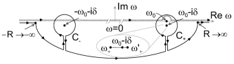
Figure 1: The complex $\omega$-plane showing the original integration path (dashed line, offset vertically for clarity) and the deformed contour of integration (solid line, offset vertically for clarity). Also shown is the singular point at $\omega=\omega_{0}-i\delta$ and the simple pole at $\omega=\omega_{0}$.

In order to facilitate the evaluation of the complex integral for the propagated field, we deform the original contour of integration (i.e., the real axis, slightly moved to leave the pole under it), to a semicircle of infinite radius in the lower complex half-plane that connects the $\pm$ real points at infinity. The value of the integral over this semicircle is zero. As the deforming contour cuts through the two obstructing branchcuts, it leaves behind two clockwise-oriented contour loops, $C_{+}$ encircling the right branchcut and $C_{-}$ encircling the left one. As shown in Fig. 1, the loops, except for their orientation, are chosen to be mirror images of each other with respect to the imaginary axis. Furthermore, $C_{+}$ is chosen to pass through the Sommerfeld and Brillouin saddle-points (i.e., stationary points of the exponential in the Fourier integral, see below) in the right half-plane. This implies that $C_{-}$ also passes through the two saddle-points in the left half-plane. Within the regime of validity of the saddle-point method, the main contributions to the integrals are localized near these saddle-points. The pole residue contribution must be added to the field if the pole $\omega_{c}$ is positioned outside $C_{+}$.

The integral over $C_{-}$, representing the so-called counter-rotating contribution to the propagated field, can be efficiently represented as an integral over $C_{+}$ through a change of the variable of integration $\omega\to-\overline{\omega}$ (bar indicates complex conjugate) and using the symmetry of the exponent,

$$\psi(-\overline{\omega})=\overline{\psi(\omega)}.$$ (8)

We thus obtain

$$\int_{C_{-}}\dfrac{e^{\psi(\omega)}}{\omega-\omega_{c}}d\omega=-\overline{\int_{C_{+}}\dfrac{e^{\psi(\omega)}}{\omega+\omega_{c}}d\omega}.$$ (9)

Inserting Eq. (9) in Eq. (1), we obtain

$$E(z,t)=E_{rot}(z,t)+E_{crot}(z,t)+\xi_{C_{+}}E_{c},$$ (10)

where the rotating term is given by

$$E_{rot}(z,t)=-\text{Re}\left(\dfrac{A_{0}\Theta(\tau)}{2\pi}\int_{C_{+}}\dfrac{e^{\psi(\omega)}}{\omega-\omega_{c}}d\omega\right),$$ (11)

the counter-rotating term is

$$E_{crot}(z,t)=\text{Re}\left(\dfrac{A_{0}\Theta(\tau)}{2\pi}\overline{\int_{C_{+}}\dfrac{e^{\psi(\omega)}}{\omega+\omega_{c}}d\omega}\right),$$ (12)

the pole contribution is

$$E_{c}=A_{0}\Theta(\tau)\mbox{e}^{-\alpha_{0}z/2}\sin\left(\omega_{0}\tau+\frac{\omega_{0}\Delta n_{r}}{c}z\right),$$ (13)

which represents the main field, and $\xi_{C_{+}}=0\ \mbox{or}\ 1$ according to whether $C_{+}$ encloses the pole or not (if the pole is enclosed, the main field is contained in $E_{rot}$). The sum of the rotating term and the third term in Eq. (10) remains constant under deformations of the contour $C_{+}$.

The expression for the main field (13) displays exponential attenuation as a function of propagation distance, which is governed by the absorption coefficient $\alpha_{0}$ at frequency $\omega_{c}=\omega_{0}$. It is defined through the relation

$$\alpha_{0}=\frac{2\omega_{0}n_{i}(\omega_{0})}{c},$$ (14)

where

$$n_{i}(\omega_{0})=\text{Im}[n(\omega_{0})].$$ (15)

The value of the refractive index at the resonant frequency is given by,

$$n(\omega_{0})=\sqrt{\frac{1+im/3}{1-im/6}},$$ (16)

or, in polar form,

$$n(\omega_{0})=2\sqrt{\frac{m^{2}+9}{m^{2}+36}}\text{e}^{i[\tan^{-1}9m/(18-m^{2})]/2},$$ (17)

where

$$m=\frac{\omega_{p}^{2}}{\omega_{0}\delta}.$$ (18)

Thus,

$$n_{i}(\omega_{0}) = \text{Im}[n(\omega_{0})]$$

$$= 2\sqrt{\frac{m^{2}+9}{m^{2}+36}}\sin\left(\frac{1}{2}\tan^{-1}\frac{9m}{18-m^{2}}\right)$$

and

$$n_{r}(\omega_{0}) = \text{Re}[n(\omega_{0})]$$

$$= 2\sqrt{\frac{m^{2}+9}{m^{2}+36}}\cos\left(\frac{1}{2}\tan^{-1}\frac{9m}{18-m^{2}}\right).$$

The main signal also experiences a $z$-dependent phase shift arising from the real part of the refractive index, where $\Delta n_{r}=n_{r}(\omega_{0})-1$. As discussed in Sec. VII, our derivation of expressions for optical precursors allows for large absorption coefficients and Eqs. (II) and (II) must be used. On the other hand, a simplified expression for the refractive index can be obtained, and a connection to other treatments of optical pulse propagation can be made when the absorption is small ($\alpha_{0}\ll\omega_{0}/c$). In this case,

$$n_{i}(\omega_{0})\simeq\frac{\omega_{p}^{2}}{4\omega_{0}\delta},$$ (21)

$$n_{r}(\omega_{0})\simeq 1,$$ (22)

$$\alpha_{0}\simeq\frac{\omega_{p}^{2}}{2c\delta},$$ (23)

$$\Delta n_{r}\simeq 0.$$ (24)

Here, we see immediately that $\alpha_{0}$ scales with $\omega_{p}^{2}$ and inversely with $\delta$.

Using Eqs. (11)-(13) in the expression for the field (10), we calculate the precursors from contributions from only the Sommerfeld and Brillouin saddle-points in the right half-plane; they include the contributions from their symmetric counterparts in the left half-plane through the second integral. Henceforth, references to saddle points or a branchcut are to the ones in the right half-plane.

In order to perform the calculation of the saddle-points explicitly, and thus obtain an explicit expression of the precursor fields, we focus on an asymptotically large material resonance frequency $\omega_{0}$. In this limit, the material is dilute ($\omega_{p}\ll\omega_{0}$) and narrowbanded ($\delta\ll\omega_{0}$). In the scale of $\omega_{0}$, the branchpoints (6) and (7) of the right half-plane ($\omega_{+}$ and $\omega_{+}^{\prime}$, respectively) collapse asymptotically to the “singular point” $\omega_{0}-i\delta$, as illustrated in Fig. 1. The more precise asymptotic formula for the midpoint of the collapsing branchcut (not needed in our calculation) is $\omega_{0}-i\delta+(\omega_{p}^{2}/12-\delta^{2}/2)/\omega_{0}$. The length $l$ of the branchcut, i.e., the difference $\omega_{+}^{\prime}-\omega_{+}$, is given asymptotically by

$$l\sim\frac{\omega_{p}^{2}}{2\omega_{0}}\ll\omega_{0}.$$ (25)

We make the singular point the center of a new frequency variable, denoted by $\omega_{*}$ and defined by

$$\omega=\omega_{0}-i\delta+\omega_{*}.$$ (26)

We seek parameters (frequency, material, depth, retarded time) for which the values of $\omega_{*}$ at the Sommerfeld and Brillouin saddle-points are at a scale that is intermediate between the large material frequency $\omega_{0}$ and the small length $l$ of the branchcut. We require

$$\frac{\omega_{p}^{2}}{2\omega_{0}}\ll\omega_{*}\ll\omega_{0}.$$ (27)

As a result, the saddle-points view the branchcut as a point. Furthermore, for near resonance excitation ($\omega_{c}\simeq\omega_{0}$), the saddle points are disproportionately farther away from the center frequency $-\omega_{0}+i\delta$ of the counter-rotating term than from the center frequency $\omega_{0}+i\delta$ of the rotating terms. Using these facts allows us to obtain explicit expressions for the precursors and for the transient field, as discussed below.

III Calculation of the precursors

In order to calculate the integrals that give the field, we seek to isolate the dominant terms in the exponent $\psi$ and, in particular, in the expression for the refractive index. The value of $a$ in Eq. (4), expressed in terms of the new frequency variable $\omega_{*}$, is

$$a=2\omega_{0}\omega_{*}+\omega_{*}^{2}+\frac{1}{3}\omega_{p}^{2}.$$ (28)

Following our scaling,

$$a\sim 2\omega_{0}\omega_{*},$$ (29)

and the term $\omega_{p}^{2}/a$ in Eq. (4) satisfies

$$\frac{\omega_{p}^{2}}{a}\sim\frac{\omega_{p}^{2}}{2\omega_{0}\omega_{*}}\ll 1.$$ (30)

Defining

$$n_{1}=\frac{\omega_{p}^{2}}{4\omega_{0}\omega_{*}},$$ (31)

we write the refractive index as

$$n=1-n_{1}+d,$$ (32)

where the error term $d$ satisfies $d=O(n_{1}^{2})$. We insert Eq. (32) in Eq. (3) for $\psi$ to obtain

$$\psi=-i\omega\tau-i\frac{z}{c}\omega(n_{1}-d).$$ (33)

where we have used the retarded time (Eq. (2)).

We insert the change of variable (26) into this expression and arrange the terms into three groups, as indicated here with the aid of braces

$$\psi=\left\{-i\omega_{0}\tau-\delta\tau\right\}+\left\{-i\omega_{*}\tau-i\frac{z}{c}\omega_{0}n_{1}\right\}$$ (34)

$$+\left\{i\frac{z}{c}\omega_{0}d-\frac{z}{c}\delta(n_{1}-d)-i\frac{z}{c}\omega_{*}(n_{1}-d)\right\}.$$

The two terms of the first group are independent of the variable of integration and give the leading amplitude and phase contributions to the integral. Our theory applies to parameters (to be identified below) for which the second group is dominant, allowing for the third group, labeled $\psi_{rem}$ (mnemonic remainder) to be neglected in the calculation of the saddle-points. The second group is further simplified by introducing the rescaled frequency variable $\eta$, defined by

$$\omega_{*}=\frac{q}{\tau}\eta,$$ (35)

where $q$ is given by

$$q=\frac{\omega_{p}}{2}\sqrt{\frac{z\tau}{c}}.$$ (36)

Using these notations, the phase is given by

$$\psi=\{-i\omega_{0}\tau-\delta\tau\}+\{-iq(\eta+\eta^{-1})\}+\psi_{rem}.$$ (37)

Inserting this expression into Eqs. (11) and (12) and changing the variable of integration to $\eta$, we obtain

$$E_{rot}(z,t)=-\text{Re}\left[\frac{A_{1}}{2\pi}\oint_{C_{+}(\eta)}\mbox{e}^{\psi_{rem}}\dfrac{\mbox{e}^{-iq(\eta+\eta^{-1})}}{\eta-i\sigma}d\eta\right],$$ (38)

$$E_{crot}(z,t)=\text{Re}\left[\frac{A_{1}}{2\pi}\oint_{C_{+}(\eta)}\mbox{e}^{\psi_{rem}}\dfrac{\mbox{e}^{-iq(\eta+\eta^{-1})}}{\eta-i\sigma+2(\omega_{c}\tau/q)}d\eta\right],$$ (39)

$$A_{1}=A_{0}\Theta(\tau)\mbox{e}^{-\delta\tau-i\tau\omega_{0}},$$ (40)

$$\sigma=2\frac{\delta}{\omega_{p}}\sqrt{\frac{c\tau}{z}},$$ (41)

where ${C_{+}(\eta)}$ is the image of the contour $C_{+}$ in the $\eta$ plane as shown in Fig. 2. We note that formulae (38) and (39) are exact, in spite of their derivation being guided by asymptotic considerations.

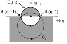
Figure 2: The complex $\eta$-plane showing contour of integration $C_{d}$ (dashed line) and the short stretches along $C_{d}$ that give the dominant contribution to the integral. The contour $C_{d}$ is a deformation of the contour $C_{3}$ (not shown for clarity). The solid line is a circle of radius 1 centered at the origin. The shaded regions are the portion of the $\eta$-plane for which the real part of the exponent of the integrand is negative.

We now turn to our calculation of the precursors, which implements the following approximations.

1. We neglect the terms of $\psi_{rem}$ altogether, i.e., we set $\psi_{rem}=0$ (see discussion in section IV). The saddle-points are then approximated as the stationary points of $\eta+\eta^{-1}$, namely, $\eta=1$ for the Sommerfeld precursor and $\eta=-1$ for the Brillouin precursor (see Fig. 2). The saddle-point approximation of the integrals is straightforward and given below. The omitted terms give only higher order contributions to the phase and amplitude of each precursor. A method for obtaining higher-order corrections is discussed in the Appendix.

2. The counter-rotating term of the field $E_{crot}$ is neglected. In our case of near-resonant excitation and with our scaling, the relative error introduced is of order $q/(\tau\omega_{0})=(\omega_{p}/\omega_{0})\sqrt{z/(c\tau)}\ll 1$ (see relation (60) below), following the fact that $|\omega_{*}|=q/\tau$ at the saddle-points.

As a result of these approximations, the propagated field is given as

$$E(z,t)=-\text{Re}\left[\frac{A_{1}}{2\pi}\oint_{C_{+}(\eta)}\dfrac{\mbox{e}^{-iq(\eta+\eta^{-1})}}{\eta-i\sigma}d\eta\right]+\Theta(\sigma-1),$$ (42)

where $C_{+}(\eta)$ is the unit circle in the $\eta$ plane (see Fig. 2).

The saddle-point method for evaluating the integral in Eq. (42) requires large values of $q$, the relative error of its approximation to the value of the integral being of order $1/q$. In order to apply the method, we deform the contour of integration $C_{+}(\eta)$ to the contour $C_{d}$ (see Fig. 2), oriented clockwise, that passes through the saddle-points $\eta=\pm 1$ cutting the real axis at angle $\pi/4$. The value that the real part of the exponent assumes at the saddle-points is maximal, in comparison to its values in the shaded region shown in the figure. The contour of integration $C_{d}$ passes through the saddle-points and stays in the shaded region. In the limit of large $q$, exponential decay in the shaded region makes the contribution of the part of the contour close to the saddle points dominant. The main contributions to the integral arise from the two short stretches of the contour $C_{d}$ in the neighborhood of the saddle points, which have been chosen in the steepest descent direction ($\pi/4$ angles with the real axis) where the exponential is purely real and the integrands are approximated by Gaussians. Large values of $q$ localize the Gaussians at the saddle-points. Thus, the length of the stretches tends to zero as $q$ increases. The contributions from the two saddle-points to the rotating term of the field, obtained from the exact calculation of the Gaussian integrals, are

$$E_{S}(z,t) = \mbox{Re}\left[\dfrac{iA_{1}\mbox{e}^{-i(2q-\frac{\pi}{4})}}{2\left({\pi q}\right)^{\frac{1}{2}}(1-i\sigma)}\right],$$ (43)

$$E_{B}(z,t) = \mbox{Re}\left[\dfrac{iA_{1}\mbox{e}^{i(2q-\frac{\pi}{4})}}{2\left({\pi q}\right)^{\frac{1}{2}}(1+i\sigma)}\right],$$ (44)

with the subscript $S\ (B)$ for the Sommerfeld (Brillouin) precursor field. Inserting Eq. (40) into these obtains the two precursor fields

$$E_{S}(z,t) = \mbox{Re}\left[\dfrac{iA_{0}\Theta(\tau)\mbox{e}^{-\delta\tau-i(2q-\frac{\pi}{4})}}{2\left({\pi q}\right)^{\frac{1}{2}}(1-i\sigma)}\mbox{e}^{-i\tau\omega_{0}}\right],$$ (45)

$$E_{B}(z,t) = \mbox{Re}\left[\dfrac{iA_{0}\Theta(\tau)\mbox{e}^{-\delta\tau+i(2q-\frac{\pi}{4})}}{2\left({\pi q}\right)^{\frac{1}{2}}(1+i\sigma)}\mbox{e}^{-i\tau\omega_{0}}\right].$$ (46)

The precursors display rapid oscillations at a frequency close to $\omega_{0}$, modulated by a complex-valued envelope. Both precursor envelopes have the same modulus

$$A_{S,B}(z,t)=\dfrac{A_{0}\Theta(\tau)\mbox{e}^{-\delta\tau}}{2\left({\pi q(1+\sigma^{2})}\right)^{\frac{1}{2}}}.$$ (47)

The precursors decay exponentially with time constant $1/\delta$, supporting our statement that they persist for a time determined by the resonance half-width, which can be in the nanosecond time scale for a dilute gas of cold atoms Jeong et al. (2006), for example. The precise value of the frequency of the Sommerfeld and Brillouin precursors is determined by taking the derivative of the phase $\tau\omega_{0}+2q$ with respect to $\tau$ in Eqs. (45) and (46), respectively, yielding

$$\omega_{S}=\omega_{0}+\frac{q}{\tau},\ \ \ \omega_{B}=\omega_{0}-\frac{q}{\tau}.$$ (48)

Note that the precursors frequencies are equal to the real part of the respective saddle points in the complex $\omega$-plane. Figure 3 shows the envelope and frequencies of the precursors using the materials parameters of the experiment of Jeong et al. Jeong et al. (2006) with $\omega_{0}=2.5\times 10^{15}$ $s^{-1}$, $\omega_{p}=3\times 10^{9}$ $s^{-1}$, $\delta=3\times 10^{7}$ $s^{-1}$, $\omega_{c}=\omega_{0}$, but with a longer medium length $z$=20 cm. It is seen that the envelop persists for many nanoseconds and that the precursor frequencies are within a few hundred MHz of the resonance within a few nanoseconds.

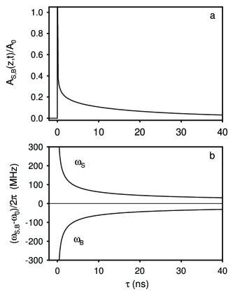
Figure 3: a) The envelope and b) frequency of the Sommerfeld and Brillouin precursors field with the medium parameters of Ref. Jeong et al. (2006) and $z=20$ cm.

The total transient field is approximated by the sum of the two precursor fields

$$E_{T}(z,t)=E_{S}(z,t)+E_{B}(z,t).$$ (49)

Because the individual precursors are chirped, $E_{T}$ will display oscillations at the beat frequency $\omega_{S}-\omega_{B}=2q/\tau$, whose period increases with $\tau$ (the beat frequency decreases with $\tau$). The envelope decays with time constant $1/\delta$ as do the individual precursors. The expression for the envelope of the total precursor field is given by

$$A_{T}(z,t)=2A_{S,B}(z,t)\textnormal{cos}(2q-\frac{\pi}{4}-\textnormal{tan}^{-1}\sigma),$$ (50)

where $q$ and $\sigma$ are given by (36) and (41), respectively. The pole, located on the imaginary axis at $i\sigma$, starts at the origin when $\tau=0$ and moves up the imaginary axis as time increases. Its contribution, i.e., the main field $E_{c}$, is negligible compared to the precursor field when the pole is in the shaded region. Outside the shaded region, the main field is dominant.

IV Parameter Analysis

The determination of the range of parameters for which our calculation of the precursors is accurate follows from assumptions we have made, which we now summarize.

1. The requirement of small $n_{1}$ in the expression for the refractive index (32) gives

   $$\frac{\omega_{p}^{2}}{2\omega_{0}\omega_{*}}\ll 1,$$ (51)

   or

   $$\frac{\omega_{p}^{2}}{2\omega_{0}}\ll\omega_{*}.$$ (52)

   This constraint is identical to the left relation (27). Inserting $\omega_{*}=q/\tau$, we obtain, after simple algebra,

   $$\frac{\omega_{p}}{\omega_{0}}\ll\sqrt{\frac{z}{c\tau}}.$$ (53)

2. The requirement of large $q$ yields the constraint

   $$\omega_{p}\gg 2\sqrt{\frac{c}{z\tau}},$$ (54)

   which can be obtained from the definition of $q$.

3. The requirement of the asymptotic vanishing of the second term of the $\psi_{rem}$ (third group of terms of Eq. (34)),

   $$\frac{z}{c}\delta(n_{1}-d)\ll 1,$$ (55)

   which, thus, does not contribute to the leading order of the integral, partly justifying our neglecting of $\psi_{rem}$. The requirement, expressed in terms of material parameters, is

   $$\frac{\omega_{p}\delta}{\omega_{0}}\sqrt{\frac{z\tau}{c}}\ll 1.$$ (56)

4. The dominance requirement constrains the remaining (first and third) terms of $\psi_{rem}$ to be significantly smaller than the terms of the second group along the contour of integration. Since the two terms of the dominant group have comparable magnitudes, it suffices to make the comparison with only the second term in the dominant group. The ratios of the first and third terms of $\psi_{rem}$ by the second term of the dominant group are, respectively,

   $$\frac{d}{n_{1}}\sim\frac{\omega_{p}^{2}}{2\omega_{0}\omega_{*}}\sim\frac{\omega_{p}}{\omega_{0}}\sqrt{\frac{c\tau}{z}}\ll 1,$$ (57)

   $$\frac{\omega_{*}}{\omega_{0}}\sim\frac{\omega_{p}}{2\omega_{0}}\sqrt{\frac{z}{c\tau}}\ll 1.$$ (58)

   These relations are identical to the scaling (left and right, respectively) of relation (27), which is thus satisfied automatically as a result of the requirement.

   By neglecting these two terms of $\psi_{rem}$, while falling short of requiring their asymptotic vanishing, we lose a phase term in the leading order expression for the precursors. That the error made is only in the phase follows from the fact that, after setting the second term of $\psi_{rem}$ equal to zero, the saddle-points are real (in the $\eta$ variable) and the exponent is purely imaginary. The dominance requirement guarantees that the error in the phase is of higher order compared to the phase correction from the second group in $\psi$ that produces the chirp. In terms of physical insight gained by our result, tolerating this error is preferable to further constraining the material parameters. The dominance requirement also guarantees there is no other leading order error in the application of the saddle-point method.

Collecting the independent constraints leaves us with

$$2\sqrt{\frac{c}{z\tau}}\ll\omega_{p}$$ (59)

for large $q$ (the requirement of a large value of $q$ is modest - the saddle-point method already gives a quite good approximation to the value of the integral for a value of $q$ of $3$ or $4$);

$$\frac{\omega_{p}}{\omega_{0}}\ll\sqrt{\frac{z}{c\tau}}$$ (60)

for $n_{1}\ll 1$ and dominance of the second group in $\psi$; and

$$\frac{\omega_{p}}{\omega_{0}}\ll\sqrt{\frac{c\tau}{z}},$$ (61)

and

$$\frac{\omega_{p}\delta}{\omega_{0}}\sqrt{\frac{z\tau}{c}}\ll 1.$$ (62)

for the asymptotic vanishing of the second term of $\psi_{rem}$.

When these constraints are satisfied, (a) the precursors exist at the specified retarded time (i.e., the calculation of the transient field as the sum of saddle-point contributions applies) and (b) our calculation of the precursors is accurate. When some constraint is violated, one of these statements may not be true. Assuming suitable fixed frequency, depth and material parameters, constraints (59) and (61) can be satisfied only past a (usually short) retarded time $\tau$. The constraints are satisfied in a time-range beyond this, until, for time large enough, constraint (60) is necessarily violated and our method loses accuracy.

The upper time-limit of validity of our constraints may be overshadowed by the additional practical constraint that $\delta\tau$ must be fairly small for the precursor to be observable. When

$$\frac{\delta^{2}}{\omega_{p}^{2}}=\frac{z}{c\tau},$$ (63)

the real exponentials multiplying the amplitudes of the precursor and of the main field, respectively, are equal. To be solidly in the regime where the precursor dominate over the main field, we require

$$\frac{\delta^{2}}{\omega_{p}^{2}}\ll\frac{z}{c\tau}.$$ (64)

Generally, when relation (59) is comfortably satisfied, but some other constraint fails, we expect that the precursors exist, but our calculation loses accuracy. To gain accuracy, we apply a corrective scheme described in the Appendix.

V Exact Evaluation of the Integral for the Approximate Field

Equation (42) gives the approximate propagated field, in which $\psi_{rem}$ and the counter-rotating terms have been ignored (the same approximations used to obtain the expression for the precursor fields). In order to make an exact calculation of the integral in this equation, we change to an angle variable of integration defined through $\eta=\exp[i(\rho+\pi/2)]$. We thus obtain

$$E(z,t)=\text{Re}\left[\frac{iA_{1}}{2\pi}\int_{-\pi}^{\pi}\dfrac{\mbox{e}^{2iq\sin\rho}}{1-\sigma\mbox{e}^{-i\rho}}d\rho\right]+\Theta(\sigma-1)E_{c}.$$ (65)

When the integrand of (65) is expanded in a series of powers of $\sigma<1$, each of the integrals in the series represents a Bessel function and the total field is given by

$$E(z,t)=\textnormal{Re}\left[iA_{1}\sum_{k=0}^{\infty}\sigma^{k}J_{k}(2q)\right],$$ (66)

where $J_{k}$ is the Bessel function of order $k$. The approximate transient field is obtained when the pole-contribution to the field (13), representing the main field, is subtracted from Eq. (66). While the ensuing expression for the transient field is exact in the limit considered here, it does not allow separating the two precursor fields and does not even make a statement about the existence of individual precursors. This is due to the fact that the definition of the precursors is tied to the application of the saddle-point method in the calculation of the field.

A similar calculation is possible when $\sigma>1$. In this case, the expansion is in powers of $\sigma^{-1}$ and the final formula is again a series of Bessel functions. Although we only have treated the case of a resonant field ($\omega_{c}=\omega_{0}$), the result for a near resonant field is obtained by inserting an imaginary part with the frequency difference in $\sigma$ and expanding in powers of $\sigma$ or $\sigma^{-1}$ according to whether $|\sigma|$ is less than or greater than unity.

In the parameter range of negligible local field effects ($\alpha_{0}\ll\omega_{0}/c$), an alternative formula for $\sigma$ is

$$\sigma=\sqrt{\frac{\delta\tau}{\alpha_{0}z/2}}.$$ (67)

Interestingly, when this expression for $\sigma$ is used, Eq. (66) is identical to that found by Crisp who used the slowly varying amplitude approximation (SVAA) (see Eq. (29) of Ref. Crisp (1970)). We derive Eq. (66) only with assumptions about the material properties; we make no assumption about the slowness of the variation of the electromagnetic field. Our formula (66) is still valid, even when the relation $\alpha_{0}\ll\omega_{0}/c$ is violated, as long as $\sigma$ is defined by Eq. (41).

VI Results

For the first time, we have derived analytic expressions for optical precursors for a material with a narrow resonance and a low oscillator number density (small plasma frequency). Our formulae are valid within explicitly specified sub-ranges of the space-time range of the existence of precursors. The latter consists of the range of points in space-time over which, field contributions to the main Fourier integral (Eq. (1)) are localized at isolated saddle-points of the complex frequency plane. Our precursor theory limits itself to such saddle points that are sufficiently close to the resonant frequency for the counter-rotating field contributions to be negligible and sufficiently far from it to allow approximating the branchcut in the refractive index by a singular point. These restrictions apply to the long tail of the precursors, i.e. after the narrow front of the transient wave has passed. The saddle-points involved are isolated. The front (it displays degenerate or near-degenerate saddle-points) and the very early tail, both requiring the counter-rotating contributions, are not addressed in this study. The exact expression of the field is written in the form of Eqs. (38), (39), (40), (41). The approximate field is given by Eq. (42), on which the saddle-point method is performed to yield the precursors (45) and (46). The space-time and material parameter constraints that define the range of validity of the derivation of the approximate field are given by the relations (59), (60), (61) and (62). The exact evaluation of the approximate field (42), in terms of Bessel functions is given by Eq. (66).

Our method can handle comparatively high number of oscillator densities, for which the condition $\alpha_{0}\ll\omega_{0}/c$ and, hence, the a priori assumption of the SVAA (slowly varying amplitude approximation) are no longer valid. Clearly, local field effects play a significant role in the expression of the main field. On the other hand, local field effects are still negligible in the expressions for the precursors. Indeed, the separation between the saddle-points and the resonant frequency is sufficiently high and the value of the refractive index at the saddle-points remains essentially unaffected. One verifies a posteriori, that the SVAA holds in the derived formulae for the precursor fields, both in time and in space. Indeed, the separation of the scales of the carrier and beat frequencies is guaranteed by the relation $\partial q/\partial\tau\ll\omega_{0}$ (equivalent to constraint (61)) and slow amplitude variation in time is guaranteed by $\delta\ll\omega_{0}$. The small variation of amplitude in space is guaranteed by relation $(1/(2q))\partial q/\partial z\ll 2\partial q/\partial z$. (equivalent to $1\ll q$). The left side of this relation is exponential attenuation, obtained from bringing the rational attenuation to the exponent as a logarithm and taking the spatial derivative. Our results are consistent, in the sense that the sum of precursors agrees with the transient field obtained from the exact evaluation of the approximate field in Eq. (42) (see Fig. 4). Our exact expression, in terms of a series of Bessel functions, is valid in the higher density regime as well and agrees with Crisp’s formula when restricted to low densities (see discussion below).

We now give an example of the predictions of the precursor theory and compare the results to the exact calculation of the field for the dilute narrowband dielectric. In particular, we use the parameters of the experiment of Jeong et al. Jeong et al. (2006) with $\omega_{0}=2.5\times 10^{15}$ $s^{-1}$, $\omega_{p}=3\times 10^{9}$ $s^{-1}$, $\delta=3\times 10^{7}$ $s^{-1}$, $\omega_{c}=\omega_{0}$. We first consider the case when the medium length is 0.2 cm, the value used in the experiment. For these parameters, relation (59) guaranteeing a large value of $q$, becomes an equality ($q$ takes the value $q=1$) at $\tau\approx 67$ ns, indicating that it takes on the order of hundreds of nanoseconds to satisfy the requirement. Figure 4a compares the transient field envelopes for the two theories. While there is some discrepancy at shorter times, the error is less than 25% for times greater than 30 ns, and very small at $67$ ns, indicating that condition (59) is rather conservative in this case. Thus, the primary contribution to the transient field is from the saddle points and hence it is reasonable to conclude that the experiments of Jeong et al. observed optical precursors. We note that they found that the exact theory agrees very well with the experimental observations.

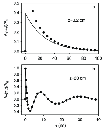
Figure 4: The envelope for the total transient field with the medium parameters of Ref. Jeong et al. (2006) and a) $z=0.2$ cm and b) $z=20$ cm. The solid line shows the predictions of the exact theory and the dots show the predictions of the asymptotic (precursor) theory.

Figure 4b compares the two theories for a medium length 100 times longer than that used in the experiment ($z$=20 cm), where it is seen that the agreement between them is excellent. The increasing-period oscillations in the transient field is clearly evident and consistent with our discussion above. In this case, $q=1$ at $\tau\approx 6.7$ ns; the good agreement at as low a value as $q=1$ again points to the conservatism of the condition (59).

VII Discussion

Crisp found that the step-modulated input field evolves toward a so-called $0\pi$ pulse whose envelope oscillates. (Note that a step-modulated incident field inherently violates the SVAA, yet our solutions are valid for this situation.) He showed that the pulse area of the total field approaches zero, which is known as a $0\pi$ pulse in the quantum optics community. Such pulses have been studied experimentally by a number of groups, beginning with the observation of Rothenberg et al. Rothenberg et al. (1984), later work demonstrating $0\pi$-pulse ‘stacking’ Ségard et al. (1987), and more recent work Matusovsky et al. (1996); Sweetser and Walmsley (1996); Dudovich et al. (2002). Crisp posed the question of whether these weak-field coherent optical transients (the $0\pi$ pulse) are a manifestation of optical precursors and answered it in the negative without mathematical proof. Certainly, Crisp explained these oscillations as an interference between the parts of the pulse spectrum above and below the atomic resonance frequency, where the central part of the spectrum is eaten away as the field propagates through the material. He did not associate these frequency components with the frequencies of the Sommerfeld and Brillouin precursors, reasoning that precursors are an ultrafast effect, which would violate the assumption of a slowly-varying amplitude, and thus must be precluded from the SVAA formalism. Our precise mathematical analysis proves conclusively that Crisp’s conclusion is incorrect. It follows clearly from our analysis that the oscillations in the envelope of the $0\pi$ pulse is the result of the interference of the Sommerfeld and Brillouin precursors.

Avenel et al. Avenel et al. (1984), on the other hand, first suggested that the coherent optical transients predicted by Crisp and observed by Rothenberg et al. Rothenberg et al. (1984) are a manifestation of optical precursors and that the time scale for the precursors can be very long (of the order of nanoseconds) for a material with a narrow resonance. However, they did not provide a mathematical justification for their claim. In later work, Varoquaux et al. Varoquaux et al. (1986) attempted to make their claim precise by solving Eq. (1) using an asymptotic method. They found a solution to the integral only for frequencies well above the frequency of the material resonance $\omega_{0}$ (see the discussion near the end of their Sec. IV.D.). They predict that the envelope of the Sommerfeld precursor contains oscillations similar in form to that predicted by Crisp, which is the same as our exact solution (Eq. (66)). They were not able to identify a Brillouin precursor. It is not surprising that they failed to obtain an accurate prediction concerning the precursors because the saddle points are located close to $\omega_{0}$ (with respect to the scale of $\omega_{0}$), yet their approximate solution to the integral only accounted for the contributions to the integral at much higher frequencies. Our calculation identifies all the saddle-point contributions to the integral and places the Avenel et al. conjecture on a firm theoretical foundation.

In addition to the calculation of the precursors, we calculated the total propagated field through the exact evaluation of the simplified Fourier integral (42). The calculation gives the total propagated field as a series of Bessel functions. This result was first obtained by Crisp Crisp (1970) under the additional assumption of the slowly varying amplitude approximation (SVAA). In the SVAA approach, the wave equation is first simplified by assuming a slowly-varying amplitude, then approximations about the material are invoked, and a solution is thus obtained. The use of a step-modulated nature of the initial field in the context of the SVAA has raised questions. The exact agreement of Crisp’s formula with our results (evaluated for a low density of oscillators), which makes no assumption of slowly varying amplitudes, demonstrates that, in spite of the initial discontinuity, the slowly-varying assumption is superficial for a weak-field and a narrow-resonance dilute medium. In fact, it can be shown that the solution to the SVAA equations for these conditions also is a solution to the full wave equation. Our derivation shows the correct way to extend Crisp’s formula to the high-density regime.

Finally, we remark that our work also has implications for very weak ‘quantum’ fields. Very recently, Du et al. Du et al. (2008a, b) have shown that precursors can be observed on long time scales in correlated bi-photon states. A follow up study considering the propagation of a classical field through a similar medium has also been presented Jeong and Du (2009).

VIII Appendix: Higher-Order Corrections

When the relation

$$\psi_{rem}\ll q(\eta+\eta^{-1})$$ (68)

does not apply comfortably, we cannot neglect $\psi_{rem}$ altogether in determining the saddle-points. Instead, we correct our calculation of each precursor by retaining the linear Taylor approximation of $\psi_{rem}$ about the corresponding saddle point. At the Sommerfeld saddle-point $\eta=1$, for example, the linear Taylor approximation of $\psi_{rem}$ is given by

$$\psi_{rem}=\gamma_{0}+\gamma_{1}\eta_{1},$$ (69)

where $\eta=1+\eta_{1}$, and $\gamma_{0}$ and $\gamma_{1}$ are the values of $\psi_{rem}$ and its first derivative at the Sommerfeld saddle-point, respectively. After letting $\eta^{-1}=(1+\eta_{1})^{-1}\approx 1-\eta_{1}+\eta_{1}^{2}$, we obtain for the exponent in (42)

$$-q(\eta+\frac{1}{\eta})\approx-q\left(2+\eta_{1}^{2}+\frac{\gamma_{0}}{q}+\frac{\gamma_{1}}{q}\eta_{1},\right),$$ (70)

for the stationary point

$$\eta_{1}=-\frac{\gamma_{1}}{2q},$$ (71)

for the exponent maximum

$$-2q-\gamma_{0}+\frac{\gamma_{1}^{2}}{4q},$$ (72)

and the second derivative at the stationary point

$$-2q.$$ (73)

In order to insert the corrections to the precursor field (45), we

1. Adjust the amplitude by multiplying the field by the factor

   $$\mbox{e}^{-\gamma_{0}+\gamma_{1}^{2}/4q},$$

   which inserts the correction of the exponent maximum (the second derivative of the exponent at the stationary point whose square root enters the fromula for the saddle-point contribution remains unchnaged in corrected exponent).

2. Perform the replacement

   $$(1-i\sigma)\rightarrow\left(1-\frac{\gamma_{1}}{2q}-i\sigma\right),$$

   in the denominator.

The calculation is similarly straightforward for the Brillouin precursor. The corrective procedure maybe iterated by using the updated saddle-point as the base point.

References

- Brillouin (1960) L. Brillouin, Wave Propagation and Group Velocity (Academic Press, New York, 1960).
- Oughstun and Sherman (1994) K. E. Oughstun and G. C. Sherman, Electromagnetic Pulse Propagation in Causal Dielectrics (Springer-Verlag, Berlin, 1994).
- Choi and Österberg (2004) S.-H. Choi and U. Österberg, Phys. Rev. Lett. 92, 193903 (2004).
- Albanese et al. (1989) R. Albanese, J. Penn, and R. Medina, J. Opt. Soc. Am. B 6, 1441 (1989).
- Roberts (2004) T. Roberts, Phys. Rev. Lett. 93, 269401 (2004).
- Alfano et al. (2005) R. Alfano, J. Birman, X. Ni, M. Alrubaiee, and B. Das, Phys. Rev. Lett. 94, 239401 (2005).
- Gibson and Österberg (2005) U. Gibson and U. Österberg, Opt. Express 13, 2105 (2005).
- Avenel et al. (1984) O. Avenel, E. Varoquaux, and G. A. Williams, Phys. Rev. Lett. 53, 2058 (1984).
- Jeong et al. (2006) H. Jeong, A. M. C. Dawes, and D. J. Gauthier, Phys. Rev. Lett. 96, 143901 (2006).
- Okawachi et al. (2007) Y. Okawachi, A. D. Slepkov, I. H. Agha, D. F. Geraghty, and A. L. Gaeta, J. Opt. Soc. Am. A 24, 3343 (2007).
- Crisp (1970) M. D. Crisp, Phys. Rev. A 1, 1604 (1970).
- Oughstun and Cartwright (2003a) K. Oughstun and N. Cartwright, Opt. Express 11, 1541 (2003a).
- Oughstun and Cartwright (2003b) K. Oughstun and N. Cartwright, Opt. Express 11, 2791 (2003b).
- Rothenberg et al. (1984) J. Rothenberg, D. Grischkowsky, and A. Balant, Phys. Rev. Lett. 53, 552 (1984).
- Ségard et al. (1987) B. Ségard, J. Zemmouri, and B. Macke, Europhys. Lett. 4, 47 (1987).
- Matusovsky et al. (1996) M. Matusovsky, B. Vaynberg, and M. Rosenbluh, J. Opt. Soc. Am. B 13, 1994 (1996).
- Sweetser and Walmsley (1996) J. Sweetser and I. Walmsley, J. Opt. Soc. Am. B 13, 601 (1996).
- Dudovich et al. (2002) N. Dudovich, D. Oron, and Y. Silberberg, Phys. Rev. Lett. 88, 123004 (2002).
- Varoquaux et al. (1986) E. Varoquaux, G. A. Williams, and O. Avenel, Phys. Rev. B 34, 7617 (1986).
- Du et al. (2008a) S. Du, P. Kolchin, C. Belthangady, G. Yin, and S. E. Harris, Phys. Rev. Lett. 100, 183603 (2008a).
- Du et al. (2008b) S. Du, C. Belthangady, P. Kolchin, G. Y. Yin, and S. E. Harris, Opt. Lett. 33, 2149 (2008b).
- Jeong and Du (2009) H. Jeong and S. Du, Phys. Rev. A 79, 011802 (2009).