Stochastic Resonance with a Single Metastable State

Abstract

We study thermal instability in NbN superconducting stripline resonators. The system exhibits extreme nonlinearity near a bifurcation, which separates a monostable zone and an astable one. The lifetime of the metastable state, which is locally stable in the monostable zone, is measure near the bifurcation and the results are compared with a theory. Near bifurcation, where the lifetime becomes relatively short, the system exhibits strong amplification of a weak input modulation signal. We find that the frequency bandwidth of this amplification mechanism is limited by the rate of thermal relaxation. When the frequency of the input modulation signal becomes comparable or larger than this rate the response of the system exhibits sub-harmonics of various orders.

Stochastic resonance (SR) is a phenomenon in which metastability in nonlinear systems is exploited to achieve amplification of weak signals Benzi et al. (1983); Gammaitoni et al. (1998); Wellens et al. (2004). SR has been experimentally demonstrated in electrical, optical, superconducting, neuronal and mechanical systems Fauve and Heslot (1983); McNamara et al. (1988); Rouse et al. (1995); Hibbs et al. (1995); Abdo et al. (2006a); Longtin et al. (1991); Levin and Miller (1996); Badzey and Mohanty (2005); Chan and Stambaugh (2006). Usually, SR is achieved by operating the system in a region in which it has more than one locally stable (metastable) steady state and its response exhibits hysteresis. Under some appropriate conditions, a weak input signal, which modulates the transition rates between these states, can lead to synchronized noise-induced transitions, allowing thus strong amplification.

In the present paper we investigate SR and amplification in a superconducting (SC) NbN stripline resonator. Contrary to previous studies, we operate the system near a bifurcation between a monostable zone, in which the system has a single metastable state, and an astable zone, in which this state ceases to exist and the system lacks any steady states. In our previous studies we have investigated several effects, e.g. strong amplification Segev et al. (2007a), noise squeezing Segev et al. (2007a), and response to optical illumination Arbel-Segev et al. (2006); Segev et al. (2006), which occur near this bifurcation, and limit cycle oscillations, which are observed in the astable zone Segev et al. (2007b, c). In the present work we investigate experimentally and theoretically the response of the system to amplitude modulated input signal, and find an unusual SR mechanism that has both properties of strong responsivity and non-hysteretic behavior. The frequency bandwidth of this mechanism is found to be limited by the rate of thermal relaxation. We find that rather unique sub-harmonics of various orders are generated when the modulation frequency becomes comparable or larger than the relaxation rate. Moreover, we measure the lifetime of the metastable state in the monostable zone near the bifurcation and compare the results with a theory.

Our experiments are performed using a novel device that integrates a narrow microbridge into a SC stripline electromagnetic resonator (see Fig. 1 $\left(\mathrm{A}\right)$). Design considerations, fabrication details as well as resonance modes calculation can be found elsewhere Arbel-Segev et al. (2006). The dynamics of our system can be captured by two coupled equations of motion, which are hereby briefly described (see Ref. Segev et al. (2007c) for a detailed derivation). Consider a resonator driven by a weakly coupled feed-line carrying an incident amplitude modulated coherent tone $b^{\mathrm{in}}=b_{0}^{\mathrm{in}}(1+a\cos(\omega_{\mathrm{m}}t))e^{-i\omega_{\mathrm{p}}t}$, where $b_{0}^{\mathrm{in}}$ is constant complex amplitude, $\omega_{\mathrm{p}}$ is the driving angular frequency, $a$ is the modulation depth, and $\omega_{\mathrm{m}}\ll$ $\omega_{\mathrm{p}}$ is the modulation frequency. The mode amplitude inside the resonator can be written as $Be^{-i\omega_{\mathrm{p}}t}$, where $B\left(t\right)$ is a complex amplitude, which is assumed to vary slowly on a time scale of $1/\omega_{\mathrm{p}}$.  In this approximation, the equation of motion of $B$ reads Yurke and Buks (2006)

$$\frac{\mathrm{d}B}{\mathrm{d}t}=\left[i\left(\omega_{\mathrm{p}}-\omega_{0}\right)-\gamma\right]B-i\sqrt{2\gamma_{1}}b^{\mathrm{in}}+c^{\mathrm{in}},$$ (1)

where $\omega_{0}$ is the angular resonance frequency and $\gamma\left(T\right)=\gamma_{1}+\gamma_{2}\left(T\right)$, where $\gamma_{1}$ is the coupling coefficient between the resonator and the feed-line and $\gamma_{2}\left(T\right)$ is the temperature dependant damping rate of the mode, and $T$ is the temperature of the microbridge. The term $c^{\mathrm{in}}$ represents an input Gaussian noise. The microbridge heat balance equation reads

$$C\frac{\mathrm{d}T}{\mathrm{d}t}=2\hslash\omega_{0}\gamma_{2}\left|B\right|^{2}-H\left(T-T_{0}\right),$$ (2)

where $C$ is the thermal heat capacity, $H$ is the heat transfer coefficient, and $T_{0}=4.2\operatorname{K}$ is the temperature of the coolant.

Coupling between Eqs. (1) and (2) originates by the dependence of the damping rate $\gamma_{2}\left(T\right)$ of the driven mode on the resistance of the microbridge Saeedkia et al. (2005), which in turn depends on its temperature. We assume the simplest case, where this dependence is a step function that occurs at the critical temperature $T_{\mathrm{c}}\simeq 10\operatorname{K}$ of the superconductor, namely $\gamma_{2}$ takes the value $\gamma_{2\mathrm{s}}$ for the SC $T<T_{\mathrm{c}}$ phase of the microbridge and $\gamma_{2\mathrm{n}}$ for the normal-conducting (NC) $T>T_{\mathrm{c}}$ phase.

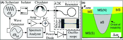
Figure 1: $\left(\mathrm{A}\right)$ Experimental setup. $\left(\mathrm{B}\right)$ System stability diagram.

Solutions of steady state response to a monochromatic excitation (no modulation $a=0$) are found by seeking stationary solutions to Eqs. (1) and (2) for the noiseless case $c^{\mathrm{in}}=0$. Due to the coupling the system may have, in general, up to two locally-stable steady-states, corresponding to the SC and NC phases of the microbridge. The stability of each of these phases depends on both the power, $P_{\mathrm{pump}}\propto$ $\left|b^{\mathrm{in}}\right|^{2}$, and frequency $\omega_{p}$ parameters of the injected pump tone. Our system has four stability zones (Fig. 1$\left(\mathrm{b}\right)$) Segev et al. (2007c). Two are mono-stable zones (MS(S) and MS(N)), where either the SC or the NC phases is locally stable, respectively. Another is a bistable zone (BiS), where both phases are locally stable Abdo et al. (2006b, c). The third is an astable zone (aS), where none of the phases are locally stable. Consequently, when the resonator is biased to this zone, the microbridge oscillates between the two phases. The onset of this instability, namely the bifurcation threshold (BT), is defined as the boundary of the astable zone (see Fig. 1$\left(\mathrm{b}\right)$).

The experimental setup is depicted in Fig. 1$(\mathrm{a})$. We inject an amplitude modulated pump tone into the resonator and measure the reflected power in the frequency domain using a spectrum analyzer and in the time domain using an oscilloscope. The parameters used for the numerical simulation were obtained as follows. The coupling coefficient $\gamma_{1}=2\operatorname{MHz}$ and the damping rates $\gamma_{2\mathrm{s}}=$ $2.2\operatorname{MHz}$, $\gamma_{2\mathrm{n}}=64\operatorname{MHz}$ were extracted from frequency response measurement Arbel-Segev et al. (2006); Abdo et al. (2006b), whereas the thermal heat capacity $C=54\operatorname{nJ}\operatorname{cm}^{-2}\operatorname{K}^{-1}$ and the heat transfer coefficient $H=12\operatorname{W}\operatorname{cm}^{-2}\operatorname{K}^{-1}$ were calculated analytically according to Refs. Johnson et al. (1996); Weiser et al. (1981).

$\begin{array}[c]{c}\text{{\parbox[b]{243.71605pt}{\begin{center} \includegraphics[height=91.13919pt,width=243.71605pt]{fig2a.eps}\\ $\left(\mathrm{A}\right)$\end{center}}}}\\ \text{{\parbox[b]{243.71605pt}{\begin{center} \includegraphics[height=182.93674pt,width=243.71605pt]{fig2b.eps}\\ $\left(\mathrm{B}\right)$\end{center}}}}\end{array}$

Figure 2: $\left(\mathrm{A}\right)$ Experimental (dotted-blue) and numerical (crossed-red) results of the signal amplification G_sig as a function of the mean injected pump power $<P_{\mathrm{pump}}>$. $\left(\mathrm{B}\right)$ Experimental (subplots $\left(x{\small 1}\right)$ and $\left(x{\small 2}\right)$) and numerical (subplots $\left(x{\small 3}\right)$ and $\left(x{\small 4}\right)$) results of the reflected power $P_{\mathrm{refl}}$ as a function of time (subplots $\left(x{\small 1}\right)$ and $\left(x{\small 3}\right)$) and scanned frequency $f_{\mathrm{SA}}$ (subplots $\left(x{\small 2}\right)$ and $\left(x{\small 4}\right)$), centered on the resonance frequency $f_{0}=4.363\mathrm{GHz}$ ($\Delta f_{\mathrm{SA}}=f_{\mathrm{SA}}-f_{0}$), where $x$ denotes $a$, $b$, and $c$, corresponding to the marked points in panel $\left(\mathrm{A}\right)$. The dashed-green curve represents the modulation signal. The time domain measurements are normalized by their maximum peak to peak value.

Our system exhibits an extremely strong amplification when tuned to the BT. Figure 2 shows both experimental (Blue curves) and numerical (Red curves) results for the case where the system is driven by a modulated pump tone having the following parameters: $\omega_{\mathrm{p}}=\omega_{0}=2\pi\times 4.363\operatorname{GHz}$, $\omega_{\mathrm{m}}=2\pi\times 10\operatorname{kHz}$, $a=0.0024$, and by an effective noise temperature of $T_{\mathrm{eff}}=75\operatorname{K}$. Panel $\left(\mathrm{A}\right)$ plots the signal gain $G_{\mathrm{sig}}$, defined as the ratio between the reflected power at frequency $\omega_{\mathrm{p}}+\omega_{\mathrm{m}}$ and the sum of the injected powers at frequencies $\omega_{\mathrm{p}}\pm\omega_{\mathrm{m}}$, as a function of the mean injected pump power $\left\langle P_{\mathrm{pump}}\right\rangle$. The system exhibits large gain of approximately $20\mathrm{dB}$ around the BT. The experimental results exhibits excess gain below BT relative to the numerical results. This can be explained by additional nonlinear mechanisms Golosovsky et al. (1995) that may induce small amplification, and are not theoretically included in our piecewise linear model.

Figure 2 $\left(\mathrm{B}\right)$, shows time and frequency domain results of the reflected power, for three pairs of input power values, corresponding to the marked points $\left(\mathrm{a-c}\right)$ in panel $\left(\mathrm{A}\right)$. In addition, the time domain measurements contain a green-dashed curve showing the modulating signal. The results shown in subplots $\left(\mathrm{a1-a4}\right)$ were obtained while biasing the system below the BT, namely, $\left\langle P_{\mathrm{pump}}\right\rangle$ was set below the power threshold, $P_{\mathrm{c}}$. In general, the spikes in the time domain plots of Fig. 2 $\left(\mathrm{B}\right)$ indicate events in which the temperature $T$ temporarily exceeds $T_{\mathrm{c}}$ Segev et al. (2007c). Below threshold, the average time between such events, which are induced by input noise, is the lifetime $\Gamma^{-1}$ of the metastable state of the resonator. As we will show in the last part of this paper, $\Gamma$ strongly depends on the pump power near BT, thus power modulation results in a modulation of the rate of spikes, as can be seen both in the experimental and simulation results.

Subplots $\left(\mathrm{b1-b4}\right)$ of Fig. 2$\left(\mathrm{B}\right)$ show experiments in which $\left\langle P_{\mathrm{pump}}\right\rangle\simeq P_{\mathrm{c}}$ and thus, the modulation itself drives the resonator in and out the astable zone. As a result, during approximately half of the modulation period nearly regular spikes in reflected power are observed, whereas during the other half only few noise-induced spikes are triggered. This behavior leads to a very strong gain as well as to the creation of higher order frequency components (subplots $\left(\mathrm{b2,b4}\right)$). Figure 2$\left(\mathrm{B}\right)$, Subplots $\left(\mathrm{c1-c4}\right)$, show experiments in which $\left\langle P_{\mathrm{pump}}\right\rangle>P_{\mathrm{c}}$, and thus the regular spikes occur throughout the modulation period. The rate of the spikes is strongly correlated to the injected power Segev et al. (2007b), and it is higher for stronger pump powers.  Therefore, as the injected pump power is modulated, so is that rate. This behavior also creates a rather strong amplification, though weaker than the one achieved in the previous case.

The amplification mechanism in our system is unique in several aspects. First it is extremely strong. To emphasize the strength of the amplification we note that, usually, no amplification greater than unity ($0~{}$dB) is achieved in such measurements with SC resonators Chin et al. (1992); Monaco et al. (2000), unless the resonator is driven near BT Thol en et al. (2007). In addition, it does not exhibit a hysteretic behavior.

$\begin{array}[c]{c}\text{{\parbox[b]{245.819pt}{\begin{center} \includegraphics[height=185.03969pt,width=245.819pt]{fig3a.eps}\\ $\left(\mathrm{A}\right)$\end{center}}}}\\ \text{{\parbox[b]{243.71605pt}{\begin{center} \includegraphics[height=75.89806pt,width=243.71605pt]{fig3b.eps}\\ $\left(\mathrm{B}\right)$\end{center}}}}\end{array}$

Figure 3: Sub-harmonics generation.

Each spike in subplots $\left(\mathrm{a1-a2}\right)$ of Fig. 2$\left(\mathrm{B}\right)$ lasts approximately $1\operatorname{\mu s}$, after which the device is ready to detect a new event. This recovery time determines the detection bandwidth. A measurement of the dependence of the amplification mechanism on the modulation frequency $\omega_{\mathrm{m}}$ has reveled a mechanism in which sub-harmonics of the modulation frequency are generated by the device. The generation occurs when the modulation period is comparable to the recovery time of the system. The results are shown in Fig. 3 which shows both experimental (Blue curves) and numerical results (Red curves) for the case of $\omega_{\mathrm{p}}=2\pi\times 4.363\operatorname{GHz}$, $a=0.017$, $T_{\mathrm{eff}}=75\operatorname{K}$, and $\omega_{\mathrm{m}}=2\pi\times 1.2\operatorname{MHz}$ for panel $\left(\mathrm{A}\right)$ and $\omega_{\mathrm{m}}=2\pi\times 2\operatorname{MHz}$ for panel $\left(\mathrm{B}\right)$. Panel $\left(\mathrm{A}\right)$, shows the reflected power, obtained for three gradually increased pump power values, and corresponding to sub-harmonics generation (SHG) of the second, third, and forth orders. SHG of the third order, for example, are generated by a quasi-periodic response of the system (subplots $\left(\mathrm{a}{\small 1},\mathrm{a}{\small 3}\right)$). Each quasi-period lasts three modulation cycles, where only during the first two a spike occurs, namely a spike is absent once every three modulation cycles. This behavior originates from the mismatch between the modulation period and the recovery time of a spike, which induces a phase difference, that is monotonically accumulated, between the two. Once every $n=3$ modulation cycles, in this case, the system fails to achieve critical conditions near the time where the peak in the modulation occurs, and therefore a spike is not triggered. Similar behavior is also shown in subplots $\left(\mathrm{a}{\small 1},\mathrm{a}{\small 3}\right)$ and $\left(\mathrm{c}{\small 1},\mathrm{c}{\small 3}\right)$, where the quasi-period lasts two and four modulation cycles respectively.

Another mechanism for SHG is observed when the modulation frequency is increased. Fig. 3, Panel $\left(\mathrm{B}\right)$, shows measurement results for $\omega_{\mathrm{m}}=2\pi\times 2\operatorname{MHz}$, which demonstrate SHG of order $n=3$. Unlike the previous case, this SHG is characterized by a single spike that occurs once every three modulation cycles.

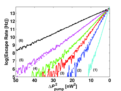
Figure 4: Escape rate of metastable states for several levels of $T_{\mathrm{eff}}$, summarized in table 1. The graphs are plotted in pairs, where the solid curves show the experimental data and the dashed curves show the corresponding theoretical fit.

We further study our system by measuring the fluctuation-induced escape rate $\Gamma$ of the metastable state in the MS(S) zone. In Ref. Abdo et al. (2007) we have found theoretically that

$$\Gamma=\Gamma_{0}\exp(-\frac{\gamma_{1}\Delta P_{\mathrm{pump}}^{2}}{\gamma^{2}k_{\mathrm{b}}T_{\mathrm{eff}}P_{\mathrm{pump}}}),$$ (3)

where $\Gamma_{0}=\sqrt{H\gamma/C}/2\pi$, and the power difference is given by $\Delta P_{\mathrm{pump}}$ $\equiv P_{\mathrm{c}}-P_{\mathrm{pump}}$. Note that the unusual scaling law in the present case $\log\left(\Gamma/\Gamma_{0}\right)\propto\Delta P_{\mathrm{pump}}^{2}$, which differs from the commonly obtained scaling low of $\log\left(\Gamma/\Gamma_{0}\right)\propto\Delta P_{\mathrm{pump}}^{3/2}$ Dykman et al. (2004); Bier (2005), is a signature of the piecewise linear dynamics of our system.

The escape rate was experimentally measured for several levels of $T_{\mathrm{eff}}$, which are given in the first row of table 1. The noise was generated by an external white noise source, and combined with the amplitude modulated pump tone. The modulation frequency was set to $500\operatorname{Hz}$, which is more than three orders of magnitude lower than the relaxation rate of the system, and therefore to a good approximation the system follows this modulation adiabatically Dykman et al. (2004).

The results are shown in Fig. 4, which plots the escape rate in logarithmic scale as a function of $\Delta P_{\mathrm{pump}}^{2}$. Six pairs of solid and dashed curves are shown, corresponding to the six different levels of injected noise intensities. The solid curves were extracted from time domain measurements of the reflected power. The dashed curves were obtained by numerically fitting the experimental data to Eq. (3) and show good quantitative agreement between the experimental results and Eq. (3). The fitting parameters included the pre-factor $\Gamma_{0}=0.86\operatorname{MHz}$ that was determined by a separate fitting process, and $P_{\mathrm{c}}$ (see table 1) that slightly decreases with the thermal noise. This behavior can be explained by local heating of the microbridge, induced by the noise that is injected into the resonator through additional resonance modes. Note that $T_{\mathrm{eff}}$ was extracted from a direct measurement of the injected noise intensity (see table 1). Note also that the system recovery time at the threshold imposes a limit on the measured escape rate. Thus the escape rate close to the threshold might be higher than measured.

Table 1: Escape rate parameters

$\ \ \begin{array}[c]{c|c|c|c|c|c|c|c}&1&2&3&4&5&6&\text{Note}\\ \hline\cr T_{\mathrm{eff}}[10^{5}\operatorname{K}]&0.52&1&1.36&1.64&2.3&3.76&\text{Measured}\\ \hline\cr P_{\mathrm{c}}^{\mathrm{fit}}[\operatorname{nW}]&125.1&121.6&120.5&120&119.2&117.6&\text{Fitted}\end{array}$

In summary, a novel mechanism of SR with a single metastable state has been demonstrated. Near BT the system exhibits rich dynamical effects including bifurcation amplification and SHG. In spite of its simplicity, our theoretical model successfully accounts for most of the experimental results.