Non local Andreev reflection in a carbon nanotube superconducting quantum interference device

Abstract

We investigate a superconducting quantum interference device (SQUID) based on carbon nanotubes in a fork geometry [J.-P. Cleuziou et al., Nature Nanotechnology 1, 53 (2006)], involving tunneling of evanescent quasiparticles through a superconductor over a distance comparable to the superconducting coherence length, with therefore “non local” processes generalizing non local Andreev reflection and elastic cotunneling. Non local processes induce a reduction of the critical current and modify the current-phase relation. We discuss arbitrary interface transparencies. Such devices in fork geometries are candidates for probing the phase coherence of crossed Andreev reflection.

I Introduction

Implementing experimentally Beckmann ; Russo ; Cadden and understanding theoretically Byers ; Deutscher ; Falci ; Samuelson ; Prada ; Koltai ; japs ; Feinberg-des ; Melin-Feinberg-PRB ; Melin-PRB ; Levy ; Duhot-Melin ; Morten ; Giazotto ; Golubov ; Zaikin ; Duhot-Melin-cond-mat ; Bouchiat ; Choi ; Martin ; Melin-Peysson ; Melin-PRB-SQUID the possibility of emitting spatially separated electron pairs from a superconductor in different electrodes has aroused considerable interest recently, in connection with the realization of a source of entangled pairs of electrons Choi ; Martin . The Josephson junction through a carbon nanotube quantum dot Delft and the superconducting quantum interference device Cleuziou (SQUID) realized recently can be viewed as steps towards future implementations of transport of spatially separated pairs of electrons in quantum information devices based on carbon nanotubes Bouchiat . As another application, the carbon nanotube SQUID realized recently by Cleuziou et al. Cleuziou in the fork geometry in Fig. 1 proves the feasibility of future measurements of magnetization reversal of individual molecular magnets.

Even more miniaturized devices may be realized in the near future, with geometrical dimensions comparable to an intrinsic length scale of the superconductor: the characteristic lengthnote-xi $\xi_{0}$ associated to the superconducting gap $|\Delta_{0}|$. Such devices Delft ; Cleuziou ; Cleuziou2 may be sensitive Byers ; Deutscher ; Falci to the fact that Andreev reflection Andreev takes place in a coherence volume of linear dimension $\xi_{0}$, therefore allowing for the possibility of splitting Cooper pairs in two parts of the circuit.

Andreev reflection Andreev is the process by which a spin-up electron incoming from the normal side on a NS interface between a normal metal N and a superconductor S is reflected as a hole in the spin-down band while a pair of electrons is transmitted in the superconductor. In a N_aSN_b structure with the electrical circuit on Fig. 2, an electron in electrode N_a can be scattered as a hole in N_b if the contacts are separated by a distance comparable to the superconducting coherence length $\xi_{0}$ (see Fig. 2a for non local Andreev reflection). Alternatively, an electron from N_a can be transmitted as an electron in N_b across the superconductor Falci (see Fig. 2b for elastic cotunneling).

The goal of our article is to address possible realizations of non local Andreev reflection in future carbon nanotube SQUIDs. These devicesMelin-Peysson ; Melin-PRB-SQUID would provide further Delft experimental signatures of the phase coherence of Cooper pair splitting. Compared to the previous Refs. [Melin-Peysson, ; Melin-PRB-SQUID, ] we investigate here higher order processes in the tunnel amplitudes giving rise to “non local Andreev bound states”. By contrast, if the distance between the Josephson junctions is much larger than the superconducting coherence length, the bound states are “local”, and localized over two separated regions of extend $\xi_{0}$ on each Josephson junction, not coupled by non local processes through the superconductor S (see Fig. 1).

The article is organized as follows. Preliminaries are presented in Sec. II. Our results are presented in Sec. III.1 for the dc-Josephson effect in single channel systems. Multichannel effects are discussed in Sec. III.2. Concluding remarks are presented in Sec. IV. Some details are left for Appendices.

II Preliminaries

II.1 Carbon nanotube superconducting interference device

A superconducting quantum interference device (SQUID) made of two superconductors and a carbon nanotube is considered (see Fig. 1a), according to the recent experiment by Cleuziou et al. Cleuziou . As a natural hypothesis, the proximity effect between the superconductor and the carbon nanotube (i.e. the penetration of pairs from the superconductor to the nanotube) is supposed to induce a minigap $|\Delta_{0}|$ in the portions of the nanotube in contact with the superconductors.

The nanotube is divided in five sections connected to each other, from top to bottom: superconducting top section with a minigap $|\Delta_{0}|$ in contact with the superconductor S’; quantum dot number 1; superconducting middle section of the nanotube with a minigap $|\Delta_{0}|$ in contact with S; quantum dot number 2; and superconducting bottom section with a minigap $|\Delta_{0}|$ in contact with the superconductor S’ (see Fig. 1a).

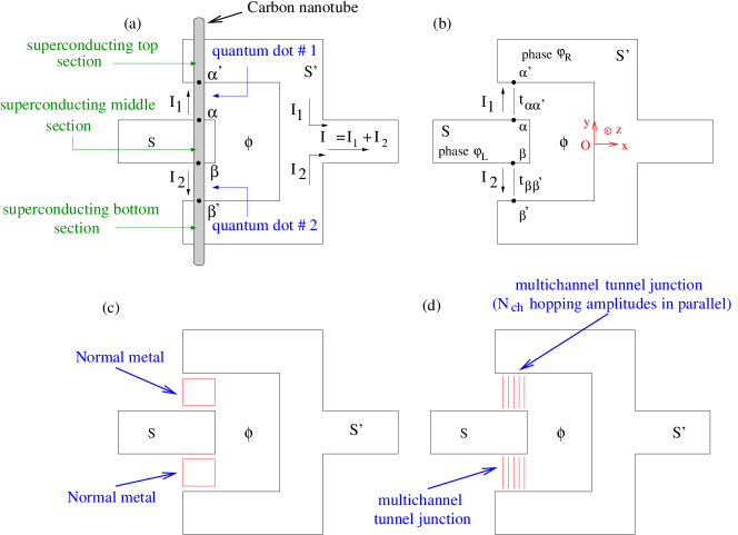
Figure 1: (Color online.) Schematic representation of the carbon nanotube SQUID (a). The hopping description in the off-resonant state is shown on (b). The transport properties of the SQUID depend only on the enclosed flux and on the superconducting phase differences, (c) shows a double bridge between two superconductors. (d) is a double insulating bridge between two superconductors, made of two multichannel insulators in parallel. Only non local processes through one of the superconductors (the superconductor S) are allowed in all these situations. The $Oxyz$ axis is shown on (b).

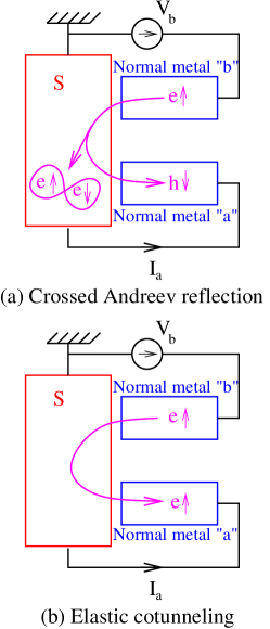
Figure 2: (Color online.) Schematic representation of the electrical circuit for probing the non local conductance in normal metal - superconductor - normal metal (N_aSN_b) structuresDelft . (a) shows a schematic representation of the non local Andreev reflection process changing a spin-up electron in electrode N_b into a spin-down hole in electrode N_a and leaving a Cooper pair in the superconductor. (b) is a schematic representation of elastic cotunneling transferring an electron from one normal electrode to the other via a trip through the superconductor.

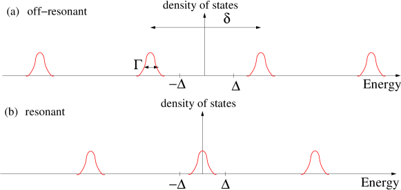
Figure 3: (Color online.) Schematic representation of quantum dot density of states, with a dot level spacing $\delta$ and a level broadening $\Gamma$. (a) corresponds to the off-resonant state considered in our article, with no resonant level in the gap window. (b) corresponds to the resonant situation with a large density of states within the gap.

Depending on the value of the gate voltage in experiments, the quantum dots 1 and 2 can be tuned from off-resonant to resonant (changing the gate voltages has the effect of shifting the dot energy levels). Our article discusses mostly the off-resonant state (in short: off-state) such that dots 1 and 2 have a vanishingly small density of states within the minigap (see Fig. 3a). It was well established experimentally by Cleuziou et al.Cleuziou that their SQUID can be tuned from the off-state with a very small critical current to the on-state with a large critical current by changing the gate voltages coupled to the two quantum dots formed by portions of the nanotube in between $\alpha$ and $\alpha^{\prime}$, and in between $\beta$ and $\beta^{\prime}$ (see Fig. 1a).

Our modeling is intended to capture “non local bound states” involving multiple electron-hole processes back and forth between dots 1 and 2. We make the following simplifying assumptions. First, proximity effect between the nanotube and the superconductor is not described explicitely on a microscopic basis: for highly transparent interfaces between the carbon nanotube and the superconductor S, we treat proximity-induced superconductivity in the nanotube as bulk superconductivity, and therefore we use the denomination “gap” instead of “minigap”. Non local processes then take place at the discontinuities of the superconducting order parameter at $\alpha$ and $\alpha^{\prime}$. For lower interface transparencies between the superconductor S and the carbon nanotube, electrons and holes may propagate in the portion of the nanotube in contact with S before undergoing non local Andreev reflection or elastic cotunneling, which amounts to averaging over many channels for non local processes.

Second, we consider the off-state with a vanishingly small density of states if the absolute value of energy is smaller than the gap (see Fig. 3a), and we use a standard description as tunnel amplitudes Caroli ; Cuevas ; Averin connecting the superconductors S and S’.

As a third assumption, it is well known that a single wall carbon nanotube contains two conduction channels. The idealized case of a single hopping amplitude is discussed in Sec. III.1. Multichannel contacts are left for Sec. III.2.

As a final assumption, Coulomb interactions in the quantum dots are not accounted for, so that $\delta$ on Fig. 3 is supposed to be a finite size effect not due to Coulomb interactions.

The distance $R_{\alpha,\beta}$ between $\alpha$ and $\beta$ (see $\alpha$ and $\beta$ on Fig. 1b) is supposed to be comparable to the coherence length $\xi_{0}$. The shortest path connecting $\alpha^{\prime}$ and $\beta^{\prime}$ (see $\alpha^{\prime}$ and $\beta^{\prime}$ on Fig. 1b) is much larger than $\xi_{0}$ ($R_{\alpha^{\prime},\beta^{\prime}}\gg\xi_{0}$), with therefore no “non local” quasiparticle tunneling between $\alpha^{\prime}$ and $\beta^{\prime}$. Compared to the fork in the experimental geometry realized in Ref. [Cleuziou, ], these assumptions on geometry can be implemented in future experiments by reducing the distance between $\alpha$ and $\beta$ (see $\alpha$ and $\beta$ on Fig. 1b) down to values comparable to the superconducting coherence length $\xi_{0}$. In the experiment by Cleuziou et al.Cleuziou , the distance $R_{\alpha,\beta}$ between $\alpha$ and $\beta$ is comparable to the distance $R_{\alpha,\alpha^{\prime}}$ between $\alpha$ and $\alpha^{\prime}$, and to the distance $R_{\beta,\beta^{\prime}}$ between $\beta$ and $\beta^{\prime}$ (of order $400$ nm). We consider on the contrary future fork geometries with $R_{\alpha,\beta}\gtrsim\xi_{0}$, and with $R_{\alpha,\beta}\ll R_{\alpha,\alpha^{\prime}},R_{\beta,\beta^{\prime}}$.

Choosing the gauge $A_{x}=-By/2$, $A_{y}=Bx/2$ and $A_{z}=0$ (with the $Oxyz$ axis on Fig. 1b), with $B$ the applied magnetic field and $\bf{A}$ the vector potential, leads to a finite value for $\int_{\alpha}^{\beta}\bf{A}\mbox{d}\bf{r}$, and to $\int_{\alpha}^{\alpha^{\prime}}\bf{A}\mbox{d}\bf{r}=-\int_{\beta}^{\beta^{\prime}}\bf{A}\mbox{d}\bf{r}$ if we suppose $R_{\alpha,\alpha^{\prime}}=R_{\beta,\beta^{\prime}}$. Given $R_{\alpha,\beta}\ll R_{\alpha,\alpha^{\prime}}$, we neglect the line integral of the vector potential between $\alpha$ and $\beta$: $\int_{\alpha}^{\beta}{\bf A}\mbox{d}{\bf r}\simeq 0$. The line integral of the vector potential along a path from $\alpha^{\prime}$ to $\beta^{\prime}$ in S’ is finite but quasiparticle propagation from $\alpha^{\prime}$ to $\beta^{\prime}$ has a vanishingly small amplitude (because $R_{\alpha^{\prime},\beta^{\prime}}\gg\xi_{0}$). Non local processes between $\alpha^{\prime}$ and $\beta^{\prime}$ are thus negligible.

II.2 Microscopic Green’s functions

The SQUID corresponds to two Josephson junctions, one for each interface. If the junctions are far apart (at a distance much larger than the superconducting coherence length), and for single channel weak links, one negative and one positive energy Andreev bound state is located on each junction, therefore leading to a total of four Andreev bound states for the SQUID (two bound states at positive energy with respect to the Fermi level, and two bound states at negative energy). As we show below, non local processes induce a coupling between these bound states in the form of level repulsion.

The supercurrent is obtained from differentiating the free energy with respect to the superconducting phase difference $\Delta\varphi$. BeenakkerBeenakker finds three terms contributing to the supercurrent, some of which date back to the early stages of Josephson junction theory Bardeen . First at zero temperature the following term corresponds to a summation over the discrete bound states within the gap:

$$I_{S}(\Delta\varphi,\phi)=\frac{2e|\Delta_{0}|}{\hbar}\sum_{n=1}^{N_{ABS}}\frac{\partial\Omega_{n}(\Delta\varphi,\phi)}{\partial(\Delta\varphi)}\theta\left[-\Omega_{n}(\Delta\varphi,\phi)\right],$$ (1)

where $\phi$ is the flux enclosed in the loop of the SQUID, and where $N_{ABS}$ is the number of Andreev bound states. The step function in energy $\theta\left[-\Omega_{n}(\Delta\varphi,\phi)\right]$ selects Andreev bound states below the Fermi level. The second term in Ref. [Beenakker, ], corresponds to the contribution of the continuum to the supercurrent. The contribution of the continuum is not included in the discussion in the forthcoming Secs. III.1 and III.2. We will justify in Sec. III.1.2 that it is indeed negligibly small in the situations that we consider. The third and last term in the expression of the supercurrent obtained by BeenakkerBeenakker vanishes if the superconducting gap is independent on the phase difference, which we assume in the following.

The bound states are obtained in a standard description as the poles of the fully dressed Green’s functions. The later is determined by the Dyson equations, which allows to describe weak links ranging from tunnel contacts to highly transparent interfaces.

The Green’s functions of the superconductor are obtained by Fourier transform in a well known procedure AGD . For superconductors isolated from each other, the local Green’s function takes the form

$$\hat{g}_{\alpha,\alpha}(\omega) = \hat{g}_{\beta,\beta}(\omega)=\frac{\pi\rho_{N}}{\sqrt{|\Delta_{0}|^{2}-(\hbar\omega)^{2}}}\left(\begin{array}[]{cc}-\hbar\omega&|\Delta_{0}|\exp(i\varphi_{L})\\ |\Delta_{0}|\exp(-i\varphi_{L})&-\hbar\omega\end{array}\right),$$ (4)

$$\hat{g}_{\alpha^{\prime},\alpha^{\prime}}(\omega) = \hat{g}_{\beta^{\prime},\beta^{\prime}}(\omega)=\frac{\pi\rho_{N}}{\sqrt{|\Delta_{0}|^{2}-(\hbar\omega)^{2}}}\left(\begin{array}[]{cc}-\hbar\omega&|\Delta_{0}|\exp(i\varphi_{R})\\ |\Delta_{0}|\exp(-i\varphi_{R})&-\hbar\omega\end{array}\right),$$ (7)

where the superconducting phase variables $\varphi_{L}$ and $\varphi_{R}=\varphi_{L}+\Delta\varphi$ are shown on Fig. 1b, $|\Delta_{0}|$ is the superconducting gap and $\rho_{N}$ the normal density of states.

The non local Green’s functions take the form

$$g_{\alpha,\beta}(\omega) = g_{\beta,\alpha}(\omega)={\cal C}(\omega)\pi\rho_{N}\left\{\frac{1}{\sqrt{|\Delta_{0}|^{2}-(\hbar\omega)^{2}}}\left(\begin{array}[]{cc}-\hbar\omega&|\Delta_{0}|\exp(i\varphi_{L})\\ |\Delta_{0}|\exp(-i\varphi_{L})&-\hbar\omega\end{array}\right)\cos{(k_{F}R_{\alpha,\beta})}\right.$$ (13)

$$\left.+\left(\begin{array}[]{cc}-1&0\\ 0&1\end{array}\right)\sin{(k_{F}R_{\alpha,\beta})}\right\},$$

where we use the notation ${\cal C}(\omega)$ for

$${\cal C}(\omega)=\exp{\left[-2\frac{R_{\alpha,\beta}}{\xi(\omega)}\right]}.$$ (14)

We parameterize below the strength of non local processes by ${\cal C}_{0}={\cal C}(\omega=0)=\exp{[-2R_{\alpha,\beta}/\xi_{0}]}$, with $\xi_{0}=\xi(\omega=0)$. The strength of non local processes is parameterized by ${\cal C}_{0}$, ranging from an absence of non local processes (${\cal C}_{0}\simeq 0$ for $R_{\alpha,\beta}\gg\xi_{0}$) to non local processes taking their maximal value (${\cal C}_{0}\simeq 1$ for $R_{\alpha,\beta}\ll\xi_{0}$). One has then the following:

$${\cal C}(\omega)=\left[{\cal C}_{0}\right]^{\xi(\omega)/\xi_{0}}.$$ (15)

Intermediate values of ${\cal C}_{0}$ are expected for a carbon nanotube with $R_{\alpha,\beta}$ of order $\xi_{0}$. Note that in the case of three dimensions (not considered here), the $\cos{(k_{F}R_{\alpha,\beta})}$ and $\sin{(k_{F}R_{\alpha,\beta})}$ factors are interchanged, and ${\cal C}(\omega)=\exp{[-2R_{\alpha,\beta}/\xi(\omega)]}/R_{\alpha,\beta}$.

The condition $R_{\alpha^{\prime},\beta^{\prime}}\gg\xi_{0}$ (see Fig. 1b) leads to

$$g_{\alpha^{\prime},\beta^{\prime}}(\omega)=g_{\beta^{\prime},\alpha^{\prime}}(\omega)=\left(\begin{array}[]{cc}0&0\\ 0&0\end{array}\right).$$ (18)

The fully dressed Green’s functions at energy $\omega$ are obtained via the Dyson equations taking the following form in a compact notation:

$$\hat{G}(\omega)=\hat{g}(\omega)+\hat{g}(\omega)\otimes\hat{\Sigma}_{t}\otimes\hat{G}(\omega),$$ (19)

where $\hat{g}(\omega)$ corresponds to the Green’s functions of the superconducting electrodes isolated from each other in the absence of tunnel amplitudes, $\hat{\Sigma}_{t}$ is the Nambu hopping self-energy, and $\hat{G}(\omega)$ is the fully dressed Green’s function. The notation $\otimes$ denotes a convolution over the network labels $\alpha$, $\beta$, $\alpha^{\prime}$ and $\beta^{\prime}$ (see the notations on Fig. 1b). For instance one has the following:

$$\hat{G}_{\alpha,\beta}(\omega)=\hat{g}_{\alpha,\beta}(\omega)+\hat{g}_{\alpha,\alpha}(\omega)\hat{t}_{\alpha,\alpha^{\prime}}\hat{G}_{\alpha^{\prime},\beta}(\omega)+\hat{g}_{\alpha,\beta}(\omega)\hat{t}_{\beta,\beta^{\prime}}\hat{G}_{\beta^{\prime},\beta}(\omega).$$ (20)

The set of fully dressed Green’s functions are then obtained from matrix inversion, and the Andreev bound states correspond to the poles within the gap. They are determined either from the corresponding analytical expressions of the Green’s functions, or from a numerical solution.

III Results

III.1 DC Josephson effect for a single transmission channel

III.1.1 Amplitude and minima of the critical current

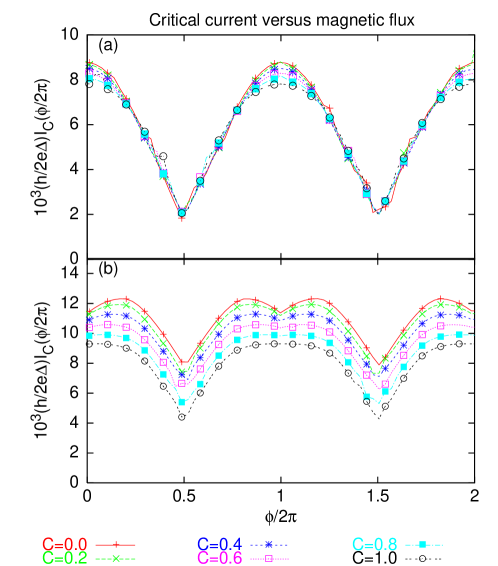
Figure 4: (Color online.) Critical current as a function of the magnetic flux $\phi$ in the loop of the SQUID, with $(T_{\alpha},T_{\beta})=(0.8,0.8)$ (a) and with $(T_{\alpha},T_{\beta})=(0.8,1)$ (b). The critical current is averaged over all values of $k_{F}R_{\alpha,\beta}$. Different curves correspond to different values of ${\cal C}_{0}$, the strength of non local processes.

We find a reduction of the supercurrent upon increasing the strength ${\cal C}_{0}$ of non local processes (see Fig. 4). On this figure, the critical current is averaged over all realizations of the Fermi phase factor $k_{F}R_{\alpha,\beta}$ corresponding to averaging over many samples with different Fermi phase factors. The interfaces of a superconducting electrode are not controlled on atomic scale and it is thus a natural assumption Falci ; Hekking to use a uniform distribution of the Fermi phase factors $k_{F}R_{\alpha,\beta}$. As expected, the reduction of the supercurrent by non local processes in a collection of single channel systems is in agreement with a collection of multichannel systems (see Sec. III.2).

Anticipating the forthcoming Sec. III.1.2, we note that non local Andreev reflection changes an electron with positive energy on one junction into a hole with negative energy on the other junction. As a consequence, bound states with positive energy are coupled to bound states with negative energies. The resulting level repulsion among bound states with opposite energies reduces in absolute value the slope of the phase dependence of the Andreev levels and therefore reduces the critical current. We evaluate in Appendix B the critical current for tunnel interfaces, and we confirm by this analytical treatment the reduction of the critical current by non local processes.

III.1.2 Level repulsion among Andreev bound states and current-phase relation

Assuming a distance between the Josephson junctions much larger than the coherence length, and assuming also single channel contacts, we find one Andreev bound state with negative energy localized on each junction, as it should. The bound states extend in the superconductor over a region of size comparable to the coherence length. If the distance between the Josephson junctions becomes comparable to the coherence length, the bound state energy levels depend on the coupling corresponding to ”non local” propagation in the superconductors (see Fig. 1).

The variations of the bound state levels ($\pm\Omega_{1}$, $\pm\Omega_{2}$) with the flux $\phi$ enclosed in the loop are shown on Fig. 5a for ${\cal C}_{0}=0$ (absence of non local processes) and on Fig. 5b for ${\cal C}_{0}=1$ (maximal value of non local processes).

Level repulsion among Andreev bound states upon increasing ${\cal C}_{0}$ (see Fig. 5b) has the effect of reducing the slope of the bound state energy levels versus phase relation, which reduces the supercurrent. The bound states take the simple form given in Appendix C (see Eqs. (32) and (33)) for a symmetric contact with $t_{a}=t_{b}$. We do not present in the article the too heavy expression of the bound state levels in the general case.

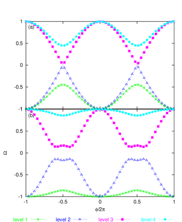
Figure 5: (Color online.) Variation of the bound state levels in the absence of non local processes (${\cal C}_{0}=0$)(a) and with the maximal strength of non local processes (${\cal C}_{0}=1$) (b). The bound states repel each other for ${\cal C}_{0}=1$ in the presence of non local processes on (b). For this figure, we use $\Delta\varphi=0$, $k_{F}R_{\alpha,\beta}=1+2\pi n$ (with $n$ an integer), $T_{\alpha}=0.8$ and $T_{\beta}=1$. A similar repulsion between Andreev bound states is obtained in the dependence of the bound state energy levels as a function of the phase difference $\Delta\varphi$.

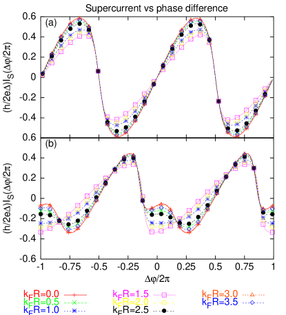
Figure 6: (Color online.) Supercurrent versus phase difference $\Delta\varphi$, with non local processes, for different values of $k_{F}R_{\alpha,\beta}$, and for $(T_{\alpha},T_{\beta})=(0.8,0.8)$, without magnetic flux $\phi=0$ (a), with magnetic flux $\phi=2$ (b). The supercurrent is very small for $k_{F}R_{\alpha,\beta}=1.5+2\pi n$ (with $n$ and integer), not far from $k_{F}R_{\alpha,\beta}\simeq\pi/2+2\pi n$.

Now we consider single channel transmission modes between the superconductors S and S’, and with non local processes at the interfaces where a step function variation of the superconducting gap is assumed. As seen from Fig. 6, the SQUID current phase relation fluctuates from sample to sample.

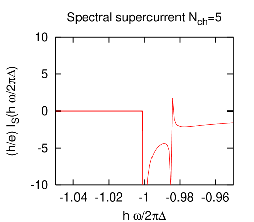
Figure 7: (Color online.) Variations of the spectral supercurrent for a given realization of the microscopic Fermi phase factors in the vicinity of $\hbar\omega=h\omega/2\pi\simeq-|\Delta_{0}|$. We find practically no contribution of the continuum for the hopping model of SQUID in the off-state. We use the phase difference $\Delta\varphi=2$ on the figure, but similar variations of the spectral current are obtained for other values of $\Delta\varphi$. We also chose ${\cal C}_{0}=1$ on the figure.

We conclude this section by discussing the contribution of the continuum Beenakker for the hopping model of SQUID in the off-state. The supercurrent is obtained as the integral over energy of the spectral supercurrent. We show on Fig. 7 a typical variation of the spectral supercurrent as a function of energy. We find practically no contribution of energies larger than $|\Delta_{0}|$ in absolute value, as opposed to other cases such as Ref. [Martin-cont, ]. We conclude that the contribution of the continuum is negligible for the hopping model of SQUID in the off-state in which the hopping elements are energy-independent. The supercurrent is therefore well approximated by Eq. (1) as in Secs. III.1 and III.2. As a physical interpretation, Andreev bound states are localized in the superconductor in a region of size set by the coherence length. A single channel weak link coupling two superconductors Cuevas is a very localized perturbation which does not couple most of the extended states in the superconducting electrodes, which explains why the states of the continuum are almost insensitive to the phase difference between the superconductors in the considered geometry with localized interfaces.

III.2 SQUIDs involving multichannel contacts

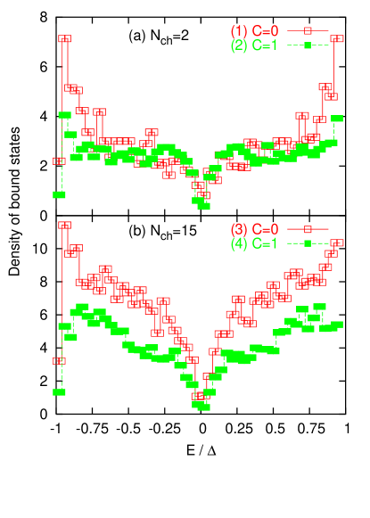
Figure 8: (Color online.) Distribution of the Andreev bound state density of states at phase difference $\Delta\varphi=\pi$, for $N_{ch}=2$ channels (a) and for $N_{ch}=15$ channels (b), without non local processes (${\cal C}_{0}=0$, $\Box$) and with non local processes to their maximal value (${\cal C}_{0}=1$, $\blacksquare$). Each histogram is normalized to the number of Andreev bound states averaged over the realizations of the Fermi phase factors.

A metallic carbon nanotube consists of two conduction channels, and it is thus natural to extend the discussion in Sec. III.1 to the case of multichannelAverin junctions (see Figs. 1c and d). We evaluate the density of Andreev bound states Lambert-ABS for multichannel systems with $N_{ch}=2$ and $N_{ch}=15$ channels, and with ${\cal C}_{0}=0$ and ${\cal C}_{0}=1$ (see Fig. 8). Increasing the strength of non local processes by increasing ${\cal C}_{0}$ reduces the density of Andreev bound states, therefore reducing the value of the supercurrent, in agreement with Sec. III.1.1.

IV Conclusions

To conclude, we have discussed signatures of non local Andreev reflection on the current-phase relation of a dc-SQUID in a fork geometry similar to Cleuziou et al.Cleuziou , but with the dimension of the middle superconductor comparable to the superconducting coherence length, so that quasiparticles may tunnel through the superconductor, with or without electron-hole conversion. Compared to a geometry consisting of two parallel normal bridges connecting two superconductors Melin-Peysson ; Melin-PRB-SQUID , we investigated here processes of higher order that are not washed out by disorder. For idealized single channel systems with sharp step-function variations of the superconducting gap in the nanotube, we found that non local processes induce sample to sample fluctuations of the current phase relation due to the dependence of non local processes on the Fermi phase factors. Multichannel systems capture moderate interface transparencies between the nanotube and the superconductor because in this case electrons incoming in the superconductor can propagate in the nanotube before undergoing crossed Andreev reflection. Increasing the strength of non local processes reduces the supercurrent, as for single channel systems.

From the point of view of future experiments, non local processes play a role in SQUIDs with fork geometries and with junctions made of carbon nanotubes, normal metals or semiconducting quantum wires. It would be interesting to measure the reduction of the current-phase relation of the SQUID upon increasing the strength of crossed processes in multichannel systems, via a comparison of samples with different dimensions, or via the temperature dependence of the coherence length. A more difficult experiment consists in probing sample to sample fluctuations of the SQUID supercurrent. A good characterization of the sample parameters (such as number of channels, interface transparencies) is required in order to distinguish between the intrinsic fluctuations of crossed processes and unwanted variations of the junction parameters when changing from one sample to another. As pointed out to us by F. Giazotto, the strength of non local processes can be monitored by the temperature dependence of the superconducting coherence length $\xi_{0}=\hbar v_{F}/|\Delta_{0}|$ (in the ballistic limit) or $\xi_{0}=\sqrt{\hbar D/|\Delta_{0}|}$ (with $D$ the diffusion coefficient in the diffusive limit) because the superconducting gap decreases with increasing temperature. Increasing temperature has thus the effect of reducing $|\Delta_{0}|$ and enhancing the coherence length. It is expected that the total amplitude of supercurrent decreases with increasing temperature, but the relative contribution of non local processes increases upon increasing temperature.

V Acknowledgments

The authors thank V. Bouchiat and W. Wernsdorffer for useful discussions on their experiments, and thank S. Florens, M. Houzet, Th. Jonckheere, Th. Martin for useful suggestions and crucial discussions. The authors thank D. Feinberg for useful discussions having resulted in this work, and for stimulating discussions.

Appendix A Fluctuations of non local transport through a diffusive superconductor

The charge transmission coefficient of a diffusive superconductor vanishes after averaging over disorder in the diffusive limit Feinberg-des ; Duhot-Melin . To show that the charge transmission coefficient of a disordered superconductor fluctuates at the scale of the Fermi wave-length $\lambda_{F}$, we show that the opposite hypothesis does not hold. Simply, we obtain fluctuations of the charge transmission coefficient by adding a very small extra ballistic region much larger than the Fermi wave-length but much smaller than the elastic mean free path.

Appendix B Critical current in the tunnel limit

In this Appendix, the supercurrent is expanded in the tunnel amplitude $t_{a,b}$ connecting the two interfaces between the superconductors. We do not detail the corresponding calculation based on diagrammatic perturbation theory. We start with the first terms of an expansion of the supercurrent in the tunnel amplitudes [see the following Eqs. (B)-(30)]. The dimensionless parameters $\tau_{a,b}=(\pi\rho_{N}t_{a,b})^{2}$, related in the tunnel limit to the dimensionless interface transparencies through $T_{a,b}\simeq 4\tau_{a,b}$, are supposed to be small. The Dyson equations are expanded systematically in the tunnel amplitudes and the lowest order diagrams are collected, leading to the following expansion for the supercurrent:

$$I_{S}(\Delta\varphi,\phi) = A_{a}\sin{(\Delta\varphi+\phi)}+A_{b}\sin{(\Delta\varphi-\phi)}+B\sin{(2\Delta\varphi)}$$

$$+ D_{a}\sin{(2(\Delta\varphi+\phi))}+D_{b}\sin{(2(\Delta\varphi-\phi))},$$

with

$$A_{a} = \frac{e}{h}\tau_{a}|\Delta_{0}|$$ (22)

$$A_{b} = \frac{e}{h}\tau_{b}|\Delta_{0}|$$ (23)

$$B = -\frac{e}{2h}\tau_{a}\tau_{b}{\cal C}_{*}^{2}|\Delta_{0}|\sin^{2}{(k_{F}R_{\alpha,\beta})}$$ (24)

$$D_{a} = -\frac{e}{2h}\tau_{a}^{2}|\Delta_{0}|$$ (25)

$$D_{b} = -\frac{e}{2h}\tau_{b}^{2}|\Delta_{0}|,$$ (26)

where ${\cal C}_{*}$ is the value of the parameter ${\cal C}(\omega)$ where $\hbar\omega$ takes the value of the bound state energy level. In this case, the bound states are very close to the gap, so that ${\cal C}_{*}\simeq 1$. The contribution of non local Andreev reflection to the supercurrent (term $B$ in Eq. (24)) is, in the tunnel limit, much smaller than the contribution of local tunneling of Cooper pairs from one superconductor to the other (terms $A_{a}$ and $A_{b}$ in Eqs. (22) and (23)).

The reduction of the supercurrent upon including non local processes is described in the tunnel limit by an expansion of Eq. (B) around $\phi=\pi/2$: $\phi=\pi/2+\delta\phi$. We consider an ensemble of single channel systems with a collection of $k_{F}R_{\alpha,\beta}$ and thus we average to $1/2$ the factor $\sin^{2}{(k_{F}R_{\alpha,\beta})}$ in Eq. (24). We define $\Delta\varphi^{(0)}$ as the value of $\Delta\varphi$ such that

$$\frac{\partial I_{S}(\Delta\varphi=\Delta\varphi^{(0)},\phi)}{\partial(\Delta\varphi)}=0,$$ (27)

and we obtain

$$\cos{(\Delta\varphi^{(0)})}=\frac{(1-\tau)\delta\phi\pm\sqrt{((1-\tau)\delta\phi)^{2}+2\tau^{2}(2-{\cal C}_{*}^{2}/2)^{2}}}{2\tau(2-{\cal C}_{*}^{2}/2)^{2}},$$ (28)

where we supposed a symmetric contact with $\tau_{a,b}=\tau$. For $\delta\phi\gg\tau$, the critical current is given by

$$I_{c}(\pi/2+\delta\phi)=4\pi\tau|\Delta_{0}|\delta\phi,$$ (29)

and for $\delta\phi\ll\tau$, it is given by

$$I_{c}(\pi/2+\delta\phi)=\pi\tau^{2}|\Delta_{0}|\left(2-\frac{{\cal C}_{*}^{2}}{2}\right).$$ (30)

For $\phi=0$ the expansion of the critical current is given by

$$I_{c}(0)=\frac{2\Delta e\tau}{h}+{\cal O}(\tau^{3}),$$ (31)

where non local effects do not enter Eq. (31) at the leading order. We conclude in the tunnel limit to a reduction of the contrast of the critical current oscillations upon increasing the strength ${\cal C}_{*}$ of non local processes. The main body of the article corresponds to interfaces with moderate of large transparencies, described by Andreev bound states obtained from the Green’s function dressed by tunnel processes to infinite order, as opposed to the limit of tunnel contacts considered in this Appendix.

Appendix C Andreev bound states

In a symmetric SQUID with $t_{a}=t_{b}$ and no magnetic field ($\phi=0$), the bound states take the form

$$\Omega^{\pm}_{1}(\Delta\varphi)=\pm|\Delta_{0}|\sqrt{A^{+}(\Delta\varphi)}/\sqrt{B^{+}(\Delta\varphi)}$$ (32)

$$\Omega^{\pm}_{2}(\Delta\varphi)=\pm|\Delta_{0}|\sqrt{A^{-}(\Delta\varphi)}/\sqrt{B^{-}(\Delta\varphi)}$$ (33)

with

$$A^{\pm}(\Delta\varphi) = 2\cos(\Delta\varphi)T\left(1\pm{\cal C}_{*}\sin(k_{F}R_{\alpha,\beta})\right)+1$$

$$+T^{2}\left(1\pm{\cal C}_{*}\sin(k_{F}R_{\alpha,\beta})\right)^{2}+T^{2}{\cal C}_{*}^{2}\cos(k_{F}R_{\alpha,\beta})^{2}$$

and

$$B^{\pm}(\Delta\varphi) = \left[1+T\left(1\pm{\cal C}_{*}\sin(k_{F}R_{\alpha,\beta})\right)\right]^{2}+T^{2}{\cal C}_{*}^{2}\cos(k_{F}R_{\alpha,\beta})^{2}$$ (35)

where $\tau=\pi^{2}\rho_{N}^{2}t^{2}=t^{2}/W^{2}$, related to the normal transmission by the relation Cuevas

$$T_{NN}^{a,b}=(4t^{2}_{a,b}/W^{2})/(1+t^{2}_{a,b}/W^{2})^{2}$$ (36)

where $W=1/\pi\rho_{N}$ is the band-width, with $\rho_{N}$ the normal density of states. The bound state levels are determined self-consistently in such a way as ${\cal C}_{*}$ is the value of ${\cal C}(\omega)$ [see Eq. (14)], where $\hbar\omega$ is replaced by the bound state energy in a self-consistent manner.

Lets us consider the case $k_{F}R_{\alpha,\beta}=2\pi n$ (with $n$ an integer). The bound states levels deduced from Eqs (C) and (35) are then degenerate:

$$\Omega^{-}_{1}(\Delta\varphi)=\Omega^{-}_{2}(\Delta\varphi)=-|\Delta_{0}|\sqrt{1-\alpha\sin(\Delta\varphi/2)^{2}}$$ (37)

with

$$\alpha = 4\tau/((1+\tau)^{2}+\tau^{2}{\cal C}_{*}^{2})=\frac{4t^{2}/W^{2}}{(1+t^{2}/W^{2})^{2}+{\cal C}_{*}^{2}t^{4}/W^{4}}.,$$ (38)

where we introduced the band-width $W$ according to Ref. [Cuevas, ]. The SQUID is then equivalent to two identical S-I-S junctions, as seen from comparing Eq. (37) to Ref. [Cuevas, ].

For $k_{F}R_{\alpha,\beta}=\pi/2+2\pi n$ (with $n$ an integer) the degeneracy is removed only if ${\cal C}_{0}\neq 0$:

$$\Omega_{1,2}^{-}(\Delta\varphi)=-|\Delta_{0}|\sqrt{1-\alpha^{(1,2)}\sin(\Delta\varphi/2)^{2}},$$ (39)

with

$$\alpha^{(1,2)}=\frac{4\tau(1\pm{\cal C}_{*})}{(1+\tau(1\pm{\cal C}_{*}))^{2}},$$ (40)

where the “$+$” and “$-$” signs correspond to “1” and “2” respectively.

In the presence of a magnetic field ($\phi\neq 0$), the bound state energy levels take the form

$$\Omega_{1,2}^{-}(\Delta\varphi)=-\tilde{|\Delta_{0}|}\sqrt{1-\alpha^{(1,2)}\sin(\Delta\varphi/2)^{2}-\beta^{(1,2)}\sin(\Delta\varphi)}$$ (41)

with

$$\alpha^{(1,2)}=\frac{4\tau\cos(2\phi)(1\pm{\cal C}_{*})}{(1+\tau(1\pm{\cal C}))^{2}-4\tau\sin(\phi)^{2}(1\mp{\cal C}_{*})\pm 4\tau^{2}{\cal C}_{*}\sin(2\phi)^{2}},$$ (42)

$$\beta^{(1,2)}=\frac{2\tau\sin(2\phi)(1\mp{\cal C}_{*})}{(1+\tau(1\pm{\cal C}))^{2}-4\tau\sin(\phi)^{2}(1\mp{\cal C}_{*})\pm 4\tau^{2}{\cal C}_{*}\sin(2\phi)^{2}}.$$ (43)

and

$$\tilde{|\Delta_{0}|}=|\Delta_{0}|\sqrt{1-4\tau\frac{\sin(\phi)^{2}(1\mp{\cal C})\pm\tau{\cal C}_{*}\sin(2\phi)^{2}}{(1+\tau(1\pm{\cal C}_{*}))^{2}}}.$$ (44)

References

- (1) D. Beckmann, H.B. Weber and H.v. Löhneysen, Phys. Rev. Lett. 93, 197003 (2004).
- (2) S. Russo, M. Kroug, T.M. Klapwijk and A.F. Morpurgo, Phys. Rev. Lett. 95, 027002 (2005).
- (3) P. Cadden-Zimansky and V. Chandrasekhar, cond-mat/0609749.
- (4) J. M. Byers and M. E. Flatté, Phys. Rev. Lett. 74, 306 (1995).
- (5) G. Deutscher and D. Feinberg, App. Phys. Lett. 76, 487 (2000);
- (6) G. Falci, D. Feinberg and F. Hekking, Europhysics Letters 54, 255 (2001).
- (7) P. Samuelsson, E.V. Sukhorukov and M. Büttiker, Phys. Rev. Lett. 91, 157002 (2003).
- (8) E. Prada and F. Sols, Eur. Phys. J. B 40, 379 (2004).
- (9) P.K. Polinák, C.J. Lambert, J. Koltai and J. Cserti, Phys. Rev. B 74, 132508 (2006).
- (10) T. Yamashita, S. Takahashi and S. Maekawa, Phys. Rev. B 68, 174504 (2003).
- (11) D. Feinberg, Eur. Phys. J. B 36, 419 (2003).
- (12) R. Mélin and D. Feinberg, Phys. Rev. B 70, 174509 (2004)
- (13) R. Mélin, Phys. Rev. B 73, 174512 (2006).
- (14) A. Levy Yeyati, F.S. Bergeret, A. Martin-Rodero and T.M. Klapwijk, cond-mat/0612027.
- (15) S. Duhot and R. Mélin, Eur. Phys. J. B 53, 257 (2006).
- (16) J.P. Morten, A. Brataas and W. Belzig, Phys. Rev. B 74, 214510 (2006).
- (17) F. Giazotto, F. Taddei, F. Beltram and R. Fazio, Phys. Rev. Lett. 97, 087001 (2006).
- (18) A. Brinkman and A.A. Golubov, Phys. Rev. B 74, 214512 (2007).
- (19) M.S. Kalenkov and A.D. Zaikin, cond-mat/0611330.
- (20) S. Duhot and R. Mélin, cond-mat/0710748.
- (21) M.S. Choi, C. Bruder and D. Loss, Phys. Rev. B 62, 13569 (2000); P. Recher,E. V. Sukhorukov and D. Loss, Phys. Rev. B 63, 165314 (2001).
- (22) G. B. Lesovik, T. Martin and G. Blatter, Eur. Phys. J. B 24, 287 (2001); N. M. Chtchelkatchev, G. Blatter, G.B. Lesovik and T. Martin, Phys. Rev. B 66, 161320(R) (2002).
- (23) V. Bouchiat, N. Chtchelkatchev, D. Feinberg, G.B. Lesovik, T. Martin and J. Torres, Nanotechnology 14, 77 (2003).
- (24) R. Mélin and S. Peysson, Phys. Rev. B 68, 174515 (2003)
- (25) R. Mélin, Phys. Rev. B 72, 134508 (2005).
- (26) P. Jarillo-Herrero, J.A. van Dam and L.P. Kouwenhoven, Nature 439, 953 (2006).
- (27) J. P. Cleuziou, W. Wernsdorfer, V. Bouchiat, T. Ondar uhu, M. Monthioux, Nature Nanotechnology 1, 53 (2006).
- (28) The coherence length at zero energy is in a ballistic system (with the Fermi velocity and the superconducting gap). In a diffusive system, , with the elastic mean free path.
- (29) J.-P. Cleuziou, W. Wernsdorfer, V. Bouchiat, Th. Ondarcuhu, M. Monthioux, cond-mat/0610622 (2006)
- (30) A.F. Andreev, Zh. Eksp. Teor. Fiz. 46, 1823 (1964) [Sov. Phys. JETP 19, 1228 (1964)].
- (31) C. Caroli, R. Combescot, P. Nozières, D. and Saint-James, J. Phys. C: Solid St. Phys. 4, 916 (1971); ibid 5, 21, (1972).
- (32) J. C. Cuevas, A. Martín-Rodero, and A. Levy Yeyati, Phys. Rev. B 54, 7366 (1996); J. C. Cuevas, A. Mart n-Rodero, and A. Levy Yeyati Phys. Rev. Lett. 82, 4086 (1999).
- (33) D. Averin and A. Bardas Phys. Rev. Lett. 75, 1831 (1995); D. Averin and H. T. Imam Phys. Rev. Lett. 76, 3814 (1996).
- (34) F.W.J. Hekking and Yu. V. Nazarov, Phys. Rev. Lett. 71, 1625 (1993); Phys. Rev. B 44, 11506 (1991).
- (35) A. Kormanyos, Z. Kaufmann, J. Cserti, C.J. Lambert, Phys. Rev. Lett. 96, 237002 (2006) and references theresin.
- (36) C.W.J. Beenakker, Phys. Rev. Lett. 67, 3836 (1991).
- (37) J. Bardeen, R. Kümmel, A.E. Jacobs and L. Tewordt, Phys. Rev. 187, 556 (1969).
- (38) A.A. Abrikosov, L.P. Gorkov and I.E. Dzyaloshinski, Methods of Quantum Field Theory in Statistical Physics (Dover, New York, 1963).
- (39) C. Benjamin, Th. Jockqueere, A. Zazunov and Th. Martin, cond-mat/0605338.