Surface plasmon polaritons and surface phonon polaritons
on metallic and semiconducting spheres:
Exact and semiclassical descriptions

Abstract

We study the interaction of an electromagnetic field with a non-absorbing or absorbing dispersive sphere in the framework of complex angular momentum techniques. We assume that the dielectric function of the sphere presents a Drude-like behavior or an ionic crystal behavior modelling metallic and semiconducting materials. We more particularly emphasize and interpret the modifications induced in the resonance spectrum by absorption. We prove that “resonant surface polariton modes” are generated by a unique surface wave, i.e., a surface (plasmon or phonon) polariton, propagating close to the sphere surface. This surface polariton corresponds to a particular Regge pole of the electric part (TM) of the $S$ matrix of the sphere. From the associated Regge trajectory we can construct semiclassically the spectrum of the complex frequencies of the resonant surface polariton modes which can be considered as Breit-Wigner-type resonances. Furthermore, by taking into account the Stokes phenomenon, we derive an asymptotic expression for the position in the complex angular momentum plane of the surface polariton Regge pole. We then describe semiclassically the surface polariton and provide analytical expressions for its dispersion relation and its damping in the non-absorbing and absorbing cases. In these analytic expressions, we more particularly exhibit well-isolated terms directly linked to absorption. Finally, we explain why the photon-sphere system can be considered as an artificial atom (a “plasmonic atom” or “phononic atom”) and we briefly discuss the implication of our results in the context of the Casimir effect.

I Introduction

In a recent article Ancey et al. (2004), we introduced the complex angular momentum (CAM) method in the context of scattering of electromagnetic waves from non-absorbing metallic and semiconducting cylinders. This allowed us to completely describe the resonant aspects of the problem in the frequency range where the dielectric function is negative. In the present article, we shall extend this analysis to non-absorbing as well as absorbing metallic and semiconducting spheres. For non-absorbing media, the transition from two dimensions to three dimensions induces some additional technical difficulties as well as the appearance of curvature correction terms in some analytic formulas describing surface polaritons (SP’s) while the physical interpretations remain quasi-identical in form. As a consequence, we will pass quickly on certain aspects lengthily analyzed in Ref. Ancey et al., 2004. By contrast, for absorbing media, different physical phenomenons occur. They can be interpreted from new correction terms (mainly due to the imaginary part of the complex dielectric constant) in the analytical expression describing the damping of SP’s.

The theory of the resonant surface polariton modes (RSPM’s) supported by metallic and semiconducting spheres has been already studied in numerous works (see, for example, Refs. Fuchs and Kliewer, 1968; Englman and Ruppin, 1968a; Ruppin and Englman, 1968; Englman and Ruppin, 1968b; Ruppin, 1982; Martinos, 1985; Ruppin, 1998; Sernelius, 2001; Dung et al., 2001; Inglesfield et al., 2004; Pitarke et al., 2007 and references therein) and is currently the subject of a renewed interest in the fields of nanotechnologies and plasmonics (for a recent comprehensive review on this subject, we refer to Ref. Atwater, 2007). In the present article, by using CAM techniquesNewton (1982); Nussenzveig (1992); W. T. Grandy (2000) in connection with modern aspects of asymptotics Dingle (1973); Berry (1989); Berry and Howls (1990); Segur et al. (1991), we shall look further into this subject. The CAM method has been extensively used in physics (we refer to the Introduction of Ref. Ancey et al., 2004 for a description of this method and for a short bibliography). We have recently introduced it in the context of electromagnetism of dispersive media (see Refs. Ancey et al., 2004, 2005, 2007). Here, by using this method, we shall provide a clear physical explanation for the excitation mechanism of the RSPM’s of the sphere as well as a simple mathematical description of the unique surface wave, i.e. of the so-called surface polariton (SP), that generates them.

Our paper is organized as follows. Section II is devoted to the exact theory: we introduce our notations, we provide the expression of the $S$ matrix of the system and we then discuss the resonant aspects of the problem. In Sec. III, by using CAM techniques, we establish the connection between the SP propagating close to the surface sphere and the associated RSPM’s. In Sec. IV, we describe semiclassically the SP by providing analytic expressions for its dispersion relation and its damping. Finally, in Sec. V, we conclude our article by explaining why the photon-sphere system can be viewed as an artificial atom (a “plasmonic atom” or “phononic atom”) and by briefly discussing the implication of our results in the context of the Casimir effect.

II Exact $S$ matrix and scattering resonances

II.1 General theory

From now on, we consider the interaction of an electromagnetic field with a metallic or semiconducting sphere with radius $a$ which is embedded in a host medium of infinite extent. In the usual spherical coordinate system $(r,\theta,\varphi)$ the sphere occupies a region corresponding to the range $0\leq r<a$ (region II) while the host medium corresponds to the range $r>a$ (region I). In the following, we implicitly assume a time dependence in $\exp(-i\omega t)$ for the electromagnetic field and we denote by $\epsilon_{c}(\omega)$ the frequency-dependent dielectric function of the sphere and by $\epsilon_{h}$ the constant dielectric function of the host medium. Furthermore, we shall use the wave numbers

$$k^{\mathrm{I}}(\omega)=\left(\frac{\omega}{c}\right)\sqrt{\epsilon_{h}}\quad\mathrm{and}\quad k^{\mathrm{II}}(\omega)=\left(\frac{\omega}{c}\right)\sqrt{\epsilon_{c}(\omega)}$$ (1)

in order to describe wave propagation in regions I and II (here $c$ is the velocity of light in vacuum).

As far as the dielectric function of the sphere is concerned, we assume it presents a Drude-like behavior Ashcroft and Mermin (1976); Fox (2001)

$$\epsilon_{c}(\omega)=\epsilon_{\infty}\left(1-\frac{\omega_{p}^{2}}{\omega^{2}+i\gamma\omega_{p}\omega}\right),$$ (2)

or an ionic crystal behavior Fuchs and Kliewer (1968); Ashcroft and Mermin (1976); Fox (2001)

$$\epsilon_{c}(\omega)=\epsilon_{\infty}\left(\frac{\omega_{L}^{2}-\omega^{2}-i\gamma\omega_{T}\omega}{\omega_{T}^{2}-\omega^{2}-i\gamma\omega_{T}\omega}\right).$$ (3)

In both cases, $\epsilon_{\infty}$ is the high-frequency limit of the dielectric function and $\gamma$ is a phenomenological damping factor. In Eq. (2), $\omega_{p}$ is the plasma frequency. In Eq. (3), $\omega_{T}$ and $\omega_{L}$ respectively denote the transverse-optical-phonon frequency and the longitudinal-optical-phonon frequency. In the first case, SP’s follow from the coupling of the electromagnetic wave with the plasma wave and are usually called surface plasmon polaritons. In the second one, SP’s follow from the coupling of the electromagnetic wave with the longitudinal and transverse acoustic waves and are usually called surface phonon polaritons. Eq. (2) can be used to describe the dielectric behavior of certain metals and semiconductors (Si, Ge, InSb, $\dots$ ) while Eq. (3) can be used to investigate the optical properties of other semiconductors such as GaAs.

In the following, we shall often consider separately the real and imaginary parts of the dielectric function. We can write

$$\epsilon_{c}(\omega)=\epsilon^{\prime}_{c}(\omega)+i\epsilon^{\prime\prime}_{c}(\omega)$$ (4)

with

$$\epsilon^{\prime}_{c}(\omega)=\epsilon_{\infty}\left[1-\frac{\omega_{p}^{2}}{\omega^{2}+(\gamma\omega_{p})^{2}}\right]$$ (5a)

$$\epsilon^{\prime\prime}_{c}(\omega)=\epsilon_{\infty}\left[\frac{\gamma\omega_{p}^{2}(\omega_{p}/\omega)}{\omega^{2}+(\gamma\omega_{p})^{2}}\right]$$ (5b)

for the Drude-like behavior and

$$\epsilon^{\prime}_{c}(\omega)=\epsilon_{\infty}\left[\frac{(\omega_{L}^{2}-\omega^{2})(\omega_{T}^{2}-\omega^{2})+(\gamma\omega_{T}\omega)^{2}}{(\omega_{T}^{2}-\omega^{2})^{2}+(\gamma\omega_{T}\omega)^{2}}\right]$$ (6a)

$$\epsilon^{\prime\prime}_{c}(\omega)=\epsilon_{\infty}\left[\frac{\gamma\omega_{T}\omega(\omega_{L}^{2}-\omega_{T}^{2})}{(\omega_{T}^{2}-\omega^{2})^{2}+(\gamma\omega_{T}\omega)^{2}}\right]$$ (6b)

for the ionic crystal behavior. It is important to note that the phenomenological damping factor $\gamma$ is always smaller than the other parameters involved in the expression of $\epsilon_{c}(\omega)$. As a consequence, we can always consider that $|\epsilon^{\prime\prime}_{c}(\omega)|\ll|\epsilon^{\prime}_{c}(\omega)|$.

The $S$ matrix of the sphere is of fundamental importance because it contains all the information about the interaction of the electromagnetic field with the sphere. It can be obtained from Maxwell’s equations and usual continuity conditions for the electric and magnetic fields at the interface between regions I and II Stratton (1941); Nussenzveig (1992); W. T. Grandy (2000). For our problem, the elements of the electric part (TM) of the $S$ matrix are given by

$$S_{\ell}^{E}(\omega)=1-2a_{\ell}^{E}(\omega)$$ (7)

with

$$a_{\ell}^{E}(\omega)=\frac{C^{E}_{\ell}(\omega)}{D^{E}_{\ell}(\omega)}$$ (8)

where $C^{E}_{\ell}(\omega)$ and $D^{E}_{\ell}(\omega)$ are two $2\times 2$ determinants which are explicitly given by

$$C_{\ell}^{E}(\omega) = k^{\text{{II}}}\left(\omega\right)\psi_{\ell}\left[k^{\text{{II}}}\left(\omega\right)a\right]\psi_{\ell}^{\prime}\left[k^{\text{{I}}}\left(\omega\right)a\right]$$ (9a)

$$\,\,-k^{\text{{I}}}\left(\omega\right)\psi_{\ell}\left[k^{\text{{I}}}\left(\omega\right)a\right]\psi_{\ell}^{\prime}\left[k^{\text{{II}}}\left(\omega\right)a\right]$$

$$D_{\ell}^{E}(\omega) = k^{\text{{II}}}\left(\omega\right)\psi_{\ell}\left[k^{\text{{II}}}\left(\omega\right)a\right]\zeta_{\ell}^{(1)^{\prime}}\left[k^{\text{{I}}}\left(\omega\right)a\right]$$ (9b)

$$\,\,-k^{\text{{I}}}\left(\omega\right)\zeta_{\ell}^{(1)}\left[k^{\text{{I}}}\left(\omega\right)a\right]\psi_{\ell}^{\prime}\left[k^{\text{{II}}}\left(\omega\right)a\right]$$

while the elements of its magnetic part (TE) are given by

$$S_{\ell}^{M}(\omega)=1-2a_{\ell}^{M}(\omega)$$ (10)

with

$$a_{\ell}^{M}(\omega)=\frac{C^{M}_{\ell}(\omega)}{D^{M}_{\ell}(\omega)}$$ (11)

where $C^{M}_{\ell}(\omega)$ and $D^{M}_{\ell}(\omega)$ are also two $2\times 2$ determinants which are now explicitly given by

$$C_{\ell}^{M}(\omega) = k^{\text{{II}}}\left(\omega\right)\psi_{\ell}\left[k^{\text{{I}}}\left(\omega\right)a\right]\psi_{\ell}^{\prime}\left[k^{\text{{II}}}\left(\omega\right)a\right]$$ (12a)

$$\,\,-k^{\text{{I}}}\left(\omega\right)\psi_{\ell}\left[k^{\text{{II}}}\left(\omega\right)a\right]\psi_{\ell}^{\prime}\left[k^{\text{{I}}}\left(\omega\right)a\right]$$

$$D_{\ell}^{M}(\omega) = k^{\text{{II}}}\left(\omega\right)\zeta_{\ell}^{(1)}\left[k^{\text{{I}}}\left(\omega\right)a\right]\psi_{\ell}^{\prime}\left[k^{\text{{II}}}\left(\omega\right)a\right]$$

$$\,\,-k^{\text{{I}}}\left(\omega\right)\psi_{\ell}\left[k^{\text{{II}}}\left(\omega\right)a\right]\zeta_{\ell}^{(1)^{\prime}}\left[k^{\text{{I}}}\left(\omega\right)a\right].$$

In Eqs. (9) and (12), we use the Ricatti-Bessel functions $\psi_{\ell}(z)$ and $\zeta_{\ell}^{(1)}(z)$ which are linked to the spherical Bessel functions $j_{\ell}(z)$ and $h^{(1)}_{\ell}(z)$ by $\psi_{\ell}(z)=zj_{\ell}(z)$ and $\zeta_{\ell}^{(1)}(z)=zh^{(1)}_{\ell}(z)$ (see Ref. Abramowitz and Stegun, 1965).

From the $S$ matrix elements, we can in particular construct the scattering cross section $\sigma_{\mathrm{sca}}$ and the absorption cross section $\sigma_{\mathrm{abs}}$ of the sphereNussenzveig (1992); W. T. Grandy (2000). They can be expressed in terms of the coefficients $a_{\ell}^{E}(\omega)$ and $a_{\ell}^{M}(\omega)$ and they are given by

$$\sigma_{\mathrm{sca}}(\omega)=\frac{2\pi}{\left[k^{\text{{I}}}\left(\omega\right)\right]^{2}}\sum_{\ell=1}^{\infty}(2\ell+1)[|a_{\ell}^{E}(\omega)|^{2}+|a_{\ell}^{M}(\omega)|^{2}]$$ (13)

and

$$\sigma_{\mathrm{abs}}(\omega)=\frac{2\pi}{\left[k^{\text{{I}}}\left(\omega\right)\right]^{2}}\sum_{\ell=1}^{\infty}(2\ell+1)\left\{[\mathrm{Re}\,a_{\ell}^{E}(\omega)-|a_{\ell}^{E}(\omega)|^{2}]\right.$$

$$\qquad\qquad\qquad\qquad\qquad\left.+[\mathrm{Re}\,a_{\ell}^{M}(\omega)-|a_{\ell}^{M}(\omega)|^{2}]\right\}.$$ (14)

From the $S$ matrix elements, we can also precisely describe the resonant behavior of the sphere as well as the geometrical and diffractive aspects of the scattering process. Here the dual structure of the $S$ matrix plays a crucial role. Indeed, the $S$ matrix is a function of both the frequency $\omega$ and the angular momentum index $\ell$. It can be analytically extended into the complex $\omega$-plane as well as into the complex $\lambda$-plane or CAM plane. (Here $\lambda$ denotes the complex angular momentum index replacing $\ell+1/2$ where $\ell$ is the ordinary momentum indexNewton (1982); Nussenzveig (1992); W. T. Grandy (2000).) The poles of the $S$ matrix lying in the fourth quadrant of the complex $\omega$-plane are the complex frequencies of the resonant modes. These resonances are determined by solving

$$D^{E,M}_{\ell}(\omega)=0\quad\mathrm{for}\quad\ell=1,2,3,\dots$$ (15)

The solutions of (15) are denoted by $\omega_{\ell p}=\omega^{(0)}_{\ell p}-i\Gamma_{\ell p}/2$ where $\omega^{(0)}_{\ell p}>0$ and $\Gamma_{\ell p}>0$, the index $p$ permitting us to distinguish between the different roots of (15) for a given $\ell$. In the immediate neighborhood of the resonance $\omega_{\ell p}$, $S^{E,M}_{\ell}(\omega)$ has the Breit-Wigner form, i.e., is proportional to

$$\frac{\Gamma_{\ell p}/2}{\omega-\omega^{(0)}_{\ell p}+i\Gamma_{\ell p}/2}.$$ (16)

The structure of the $S$ matrix in the complex $\lambda$-plane allows us, by using integration contour deformations, Cauchy’s Theorem and asymptotic analysis, to provide a semiclassical description of scattering in terms of rays (geometrical and diffracted). In that context, the poles of the $S$-matrix lying in the CAM plane (the so-called Regge poles) are associated with diffraction. They are determined by solving

$$D^{E,M}_{\lambda-1/2}(\omega)=0\quad\mathrm{for}\quad\omega>0.$$ (17)

Of course, when a connection between these two faces of the $S$ matrix can be established, resonance aspects are then semiclassically interpreted.

In the following, we shall present some numerical results. We have chosen to restrict ourselves to particular configurations, i.e., to particular values of the parameters $\epsilon_{h}$, $\epsilon_{\infty}$, $\omega_{p}$, $\omega_{T}a/c$, $\omega_{L}a/c$ and $\gamma$. These values are physically realistic or, more precisely, of the same order than physically realistic values (see, for example, Refs. Fuchs and Kliewer, 1968; Ashcroft and Mermin, 1976). In fact, even for different configurations, the results we have numerically obtained and that we shall discuss in this paper remain valid.

II.2 Sphere with a Drude-like behavior

In Figs. 1 and 2, we consider the resonant aspects of a sphere embedded in vacuum ($\epsilon_{h}=1$) and we assume that its dielectric function presents the Drude-like behavior given by Eq. (2) with $\epsilon_{\infty}=1$ and $\omega_{p}a/c=2\pi$. We examine both the non-absorbing case with $\gamma=0$ in Fig. 1 and the absorbing case with $\gamma=1/100$ in Fig. 2. In the non-absorbing case, we display the scattering cross section in Fig. 1a and, in the absorbing case, we display the absorption cross section in Fig. 2a. These cross sections are both plotted as functions of the reduced frequency $\omega a/c$. On the two figures, rapid variations of sharp characteristic shapes can be observed. This strongly fluctuating behavior is due to scattering resonances: when a pole of the $S$ matrix is sufficiently close to the real axis in the complex $\omega$-plane, it has a strong influence on the cross section [see Eq. (16)]. In Figs. 1b and 2b, resonances are exhibited for the two configurations previously considered. A one-to-one correspondence between the peaks of the cross sections and the resonances near the real $\omega a/c$-axis can be clearly observed in certain frequency ranges.

More precisely and more generally, for the dielectric function (2) there exists in the frequency range where $\epsilon^{\prime}_{c}(\omega)<0$ (i.e., where $\omega\lesssim\omega_{p}$ if we neglect terms in $\gamma^{2}$) a family of resonances associated with $S^{E}$ (TM resonances). They are close to the real axis of the complex $\omega$-plane and they converge, for large $\ell$, to the limiting complex frequency $\omega_{s}$ satisfying

$$\epsilon_{c}(\omega_{s})+\epsilon_{h}=0.$$ (18)

The real and imaginary parts of $\omega_{s}$ are easily found perturbatively by inserting

$$\omega_{s}=\omega^{\prime}_{s}+i\omega^{\prime\prime}_{s}$$ (19)

into (18) and by taking into account (4) with $|\epsilon^{\prime\prime}_{c}(\omega)|\ll|\epsilon^{\prime}_{c}(\omega)|$. By assuming that $|\omega^{\prime\prime}_{s}|\ll\omega^{\prime}_{s}$ and by using a first-order Taylor series expansion of $\epsilon_{c}(\omega_{s})$, we find that $\omega^{\prime}_{s}$ must satisfy

$$\epsilon^{\prime}_{c}(\omega_{s}^{\prime})+\epsilon_{h}=0.$$ (20a)

and that

$$\omega^{\prime\prime}_{s}=-\left.\frac{\epsilon^{\prime\prime}_{c}(\omega)}{d\ \mathrm{Re}\,\epsilon^{\prime}_{c}(\omega)/d\omega}\right|_{\omega=\omega^{\prime}_{s}}$$ (20b)

By using Eqs. (5a) and (5b) and by neglecting terms in $\gamma^{2}$, we then obtain

$$\omega^{\prime}_{s}\approx\frac{\omega_{p}}{\sqrt{1+\epsilon_{h}/\epsilon_{\infty}}}$$ (21a)

$$\omega^{\prime\prime}_{s}\approx-\frac{\gamma\omega_{p}}{2}.$$ (21b)

The general formulas (21a) and (21b) describe very well the accumulation of resonances observed in Figs. 1b and 2b in the frequency range where $\epsilon^{\prime}_{c}(\omega)<0$. It is important to note the existence of a shift in the imaginary part of the resonance spectrum [see Eq. (21b)]. It is well highlighted in Fig. 2b. It is associated with absorption and proportional to the phenomenological damping factor $\gamma$. At first sight, it can appear surprising that it does not depend on the dielectric constants $\epsilon_{\infty}$ and $\epsilon_{h}$. In fact, such a dependence only appears by working at higher orders in the perturbative expansion used.

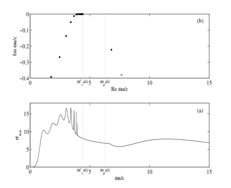
Figure 1: a) Scattering cross section $\sigma_{\mathrm{sca}}$. b) Scattering resonances in the complex $\omega a/c$-plane. We consider a non-absorbing sphere: $\epsilon_{c}(\omega)$ has the Drude type behavior with $\epsilon_{\infty}=1$, $\omega_{p}a/c=2\pi$ and $\gamma=0$ while $\epsilon_{h}=1$. Dots $(\cdot)$ correspond to poles of $S^{E}(\omega)$ while plus ($+$) correspond to poles of $S^{M}(\omega)$.

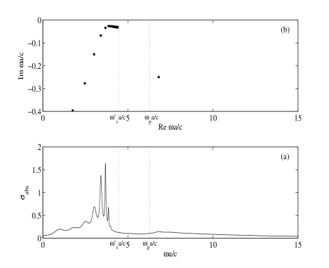
Figure 2: a) Absorption cross section $\sigma_{\mathrm{abs}}$. b) Scattering resonances in the complex $\omega a/c$-plane. We consider an absorbing sphere: $\epsilon_{c}(\omega)$ has the Drude type behavior with $\epsilon_{\infty}=1$, $\omega_{p}a/c=2\pi$ and $\gamma=1/100$ while $\epsilon_{h}=1$. Dots $(\cdot)$ correspond to poles of $S^{E}(\omega)$ while plus ($+$) correspond to poles of $S^{M}(\omega)$.

The resonances we have just considered are associated with the electric part $S^{E}$ of the $S$ matrix and they correspond to TM resonant modes of the sphere whose excitation frequencies belong to the frequency range in which $\epsilon^{\prime}_{c}(\omega)<0$. From now on (i.e., in Secs. III and IV), we shall more particularly focus our attention on the physical interpretation of these resonant modes. We shall prove that the corresponding resonances are generated by an exponentially attenuated SP propagating close to the sphere surface, this fact justifying the term RSPM’s used to denote the associated resonant modes. Furthermore, we shall show that the SP is the analog, in the large radius limit, to that supported by the plane interface. Of course, there also exists, in the whole frequency range, other families of resonances with “higher” imaginary parts and which are associated with both the electric and the magnetic parts of the $S$ matrix. They correspond to the excitation of TM and TE resonant modes of the sphere. From a physical point of view, these modes are less interesting due to their shorter lifetime. Indeed, in the new field of plasmonics, those are the SP’s with long propagation lengths and therefore very small attenuations that are especially interesting from the point of view of practical applications. Furthermore, if we consider the system photon-sphere as an artificial atom for which the photon plays the usual role of the electron (a point of view we shall push farther in Secs. III and IV), we must then keep in mind that, in the scattering of a photon with frequency $\omega^{(0)}_{\ell p}$, a decaying state (i.e., a quasibound state) of the photon-sphere system is formed. It has a finite lifetime proportional to $1/\Gamma_{\ell p}$. The resonant states whose complex frequencies belong to the family generated by the SP are therefore the most interesting because they are very long-lived states.

II.3 Sphere with an ionic crystal behavior

In Figs. 3 and 4, we consider the resonant aspects of a sphere embedded in vacuum ($\epsilon_{h}=1$) and we assume that its dielectric function presents the ionic crystal behavior given by Eq. (3) with $\epsilon_{\infty}=2$, $\omega_{T}a/c=2\pi$ and $\omega_{L}a/c=3\pi$. We examine both the non-absorbing case with $\gamma=0$ in Fig. 3 and the absorbing case with $\gamma=1/100$ in Fig. 4. In the non-absorbing case, we display the scattering cross section in Fig. 3a and, in the absorbing case, we display the absorption cross section in Fig. 4a. In Figs. 3b and 4b, resonances are exhibited for the two configurations. A one-to-one correspondence between the peaks of the cross sections and the resonances near the real $\omega a/c$-axis can be clearly observed in certain frequency ranges.

Here again, we focus our attention on the resonances existing in the frequency range where $\epsilon^{\prime}_{c}(\omega)<0$ (i.e., where $\omega_{T}\lesssim\omega\lesssim\omega_{L}$ if we neglect terms in $\gamma^{2}$). There is a family of resonances associated with $S^{E}$ (TM resonances) close to the real axis of the complex $\omega$-plane. They converge, for large $\ell$, to the limiting complex frequency $\omega_{s}$ still satisfying Eq. (18) with $\epsilon_{c}$ now given by Eq. (3). The real and imaginary parts of $\omega_{s}=\omega^{\prime}_{s}+i\omega^{\prime\prime}_{s}$ can be obtained perturbatively and we have

$$\omega^{\prime}_{s}\approx\sqrt{\frac{\omega_{L}^{2}+(\epsilon_{h}/\epsilon_{\infty})\omega_{T}^{2}}{1+\epsilon_{h}/\epsilon_{\infty}}}$$ (22a)

$$\omega^{\prime\prime}_{s}\approx-\frac{\gamma\omega_{T}}{2}.$$ (22b)

The general formulas (22a) and (22b) describe very well the accumulation of resonances observed in Figs. 3b and 4b in the frequency range where $\epsilon^{\prime}_{c}(\omega)<0$ as well as the shift in the imaginary part of the resonance spectrum.

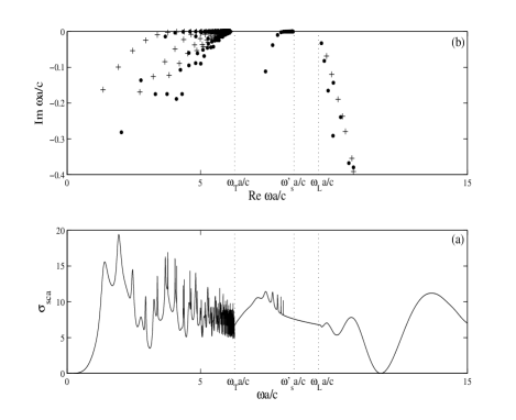
Figure 3: a) Scattering cross section $\sigma_{\mathrm{sca}}$. b) Scattering resonances in the complex $\omega a/c$-plane. We consider a non-absorbing sphere: $\epsilon_{c}(\omega)$ has the ionic crystal behavior with $\epsilon_{\infty}=2$, $\omega_{T}a/c=2\pi$, $\omega_{L}a/c=3\pi$ and $\gamma=0$ while $\epsilon_{h}=1$. Dots $(\cdot)$ correspond to poles of $S^{E}(\omega)$ while plus ($+$) correspond to poles of $S^{M}(\omega)$.

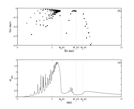
Figure 4: a) Absorption cross section $\sigma_{\mathrm{abs}}$. b) Scattering resonances in the complex $\omega a/c$-plane. We consider an absorbing sphere: $\epsilon_{c}(\omega)$ has the ionic crystal behavior with $\epsilon_{\infty}=2$, $\omega_{T}a/c=2\pi$, $\omega_{L}a/c=3\pi$ and $\gamma=1/100$ while $\epsilon_{h}=1$. Dots $(\cdot)$ correspond to poles of $S^{E}(\omega)$ while plus ($+$) correspond to poles of $S^{M}(\omega)$.

In Secs. III and IV, we shall provide a physical interpretation of the family of resonances we have just considered and we shall prove that these resonances are generated by an exponentially attenuated SP propagating close to the sphere surface and analog, in the large radius limit, to that supported by the plane interface. Of course, there also exists other families of resonances but we shall not focus our attention on them even if they seem to us physically interesting due to their rather “low” imaginary parts (see the frequency range $\omega a/c\lesssim\omega_{T}a/c$ in Figs. 3b and 4b). In fact, it is not possible to interpret them in term of SP’s analog to that supported by the plane interface because, in frequency ranges where $\epsilon^{\prime}_{c}(\omega)>0$, no surface wave can be supported by the plane interface. We think however that a semiclassical description could be achieved (maybe in terms of whispering-gallery-type surface waves) but it is out of the scope of the present work.

II.4 Comparison between cylinders and spheres

We conclude this section by making a brief comparison with the results obtained in our previous study concerning metallic and semiconducting cylindersAncey et al. (2004). Of course, in Ref. Ancey et al., 2004 we have only considered non-absorbing cylinders. As a consequence, a comparison between cylinders and spheres can be achieved only in this restricted context and we can then notice that the cross sections for the cylinders and the spheres as well as the spectra of resonances are rather similar. However, it should be noted that in the scattering by a sphere both the TM and TE polarizations contribute to the cross section (we recall that for the cylinder, the two polarizations can be studied separately) and it is important to note that, for both scatterers, SP’s and their associated RSPM’s correspond to only one polarization (the TE polarization for the cylinder and the TM polarization for the sphere). Of course, these last results remain valid even in the presence of absorption.

III Semiclassical analysis: From the SP Regge pole to the complex frequencies of RSPM’s

As already mentioned in Sec. II (see also Refs. Newton, 1982; Nussenzveig, 1992; W. T. Grandy, 2000), in the CAM approach, Regge poles determined by solving Eq. (17) are crucial to describe diffraction as well as resonance phenomenons in terms of surface waves. From the Regge trajectory associated with the SP supported by the metallic or semiconducting sphere, i.e., from the curve $\lambda_{\mathrm{SP}}=\lambda_{\mathrm{SP}}(\omega)$ traced out in the CAM plane by the corresponding Regge pole as a function of the frequency, we can more particularly deduce:

(i) the dispersion relation

$$k_{\mathrm{SP}}(\omega)=\frac{\mathrm{Re}\,\lambda_{\mathrm{SP}}(\omega)}{a}$$ (23)

of the SP which connects its wave number $k_{\mathrm{SP}}$ with the frequency $\omega$,

(ii) the damping $\mathrm{Im}\,\lambda_{\mathrm{SP}}(\omega)$ of the SP,

(iii) the phase velocity $v_{p}$ as well as the group velocity $v_{g}$ of the SP given by

$$v_{p}=\frac{\omega a}{\mathrm{Re}\,\lambda_{\mathrm{SP}}(\omega)}\quad\mathrm{and}\quad v_{g}=\frac{d~{}\omega a}{d~{}\mathrm{Re}\,\lambda_{\mathrm{SP}}(\omega)},$$ (24)

(iv) the semiclassical formula (a Bohr-Sommerfeld type quantization condition) which provides the location of the excitation frequencies $\omega^{(0)}_{\ell\mathrm{SP}}$ of the resonances generated by the SP:

$$\mathrm{Re}\,\lambda_{\mathrm{SP}}(\omega^{(0)}_{\ell\mathrm{SP}})=\ell+1/2\qquad\ell=1,2,\dots,$$ (25)

(v) the semiclassical formula which provides the widths of these resonances

$$\frac{\Gamma_{\ell\mathrm{SP}}}{2}=\left.\frac{\mathrm{Im}\,\lambda_{\mathrm{SP}}(\omega)(d\mathrm{Re}\,\lambda_{\mathrm{SP}}(\omega)/d\omega)}{(d\mathrm{Re}\,\lambda_{\mathrm{SP}}(\omega)/d\omega)^{2}+(d\mathrm{Im}\,\lambda_{\mathrm{SP}}(\omega)/d\omega)^{2}}\right|_{\omega=\omega^{(0)}_{\ell\mathrm{SP}}}$$ (26)

and which reduces to

$$\frac{\Gamma_{\ell\mathrm{SP}}}{2}=\left.\frac{\mathrm{Im}\,\lambda_{\mathrm{SP}}(\omega)}{d\ \mathrm{Re}\,\lambda_{\mathrm{SP}}(\omega)/d\omega}\right|_{\omega=\omega^{(0)}_{\ell\mathrm{SP}}}$$ (27)

in the frequency range where the condition $|d\mathrm{Re}\,\lambda_{\mathrm{SP}}(\omega)/d\omega|\gg|d\mathrm{Im}\,\lambda_{\mathrm{SP}}(\omega)/d\omega|$ is satisfied. All these results can be established by generalizing, mutatis mutandis, our approach and our calculations developed in Refs.Ancey et al., 2004, 2005 for dispersive cylinders. The transition from the dimension 2 to the dimension 3 induces some additional technical difficulties (vectorial treatment, existence of a caustic, asymptotics for spherical harmonics …) which can be rather easily overcome following and extending the works of Newton in quantum mechanics (see Ch. 13 of Ref. Newton, 1982) and the works of NussenzveigNussenzveig (1992) and GrandyW. T. Grandy (2000) in electromagnetism of ordinary dielectric media.

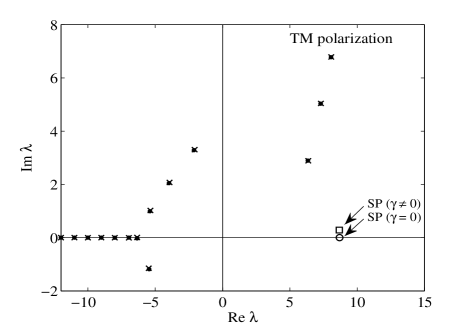
Figure 5: Regge poles in the complex angular momentum plane. $\epsilon_{c}(\omega)$ has the Drude type behavior with $\epsilon_{\infty}=1$ and $\omega_{p}a/c=2\pi$ while $\epsilon_{h}=1$. The distribution corresponds to $\omega a/c=4$ and we have $\epsilon^{\prime}_{c}(\omega)<0$. Dots $(\cdot)$ and crosses ($\mathrm{x}$) correspond respectively to Regge poles for $\gamma=0$ and for $\gamma=1/100$.

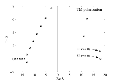
Figure 6: Regge poles in the complex angular momentum plane. $\epsilon_{c}(\omega)$ has the ionic crystal behavior with $\epsilon_{\infty}=2$, $\omega_{T}a/c=2\pi$ and $\omega_{L}a/c=3\pi$ while $\epsilon_{h}=1$. The distribution corresponds to $\omega a/c=8.3$ and we have $\epsilon^{\prime}_{c}(\omega)<0$. Dots $(\cdot)$ and crosses ($\mathrm{x}$) correspond respectively to Regge poles for $\gamma=0$ and for $\gamma=1/100$.

Figs. 5 and 6 exhibit the distribution of Regge poles for a sphere embedded in vacuum when $\epsilon^{\prime}_{c}(\omega)<0$. We only consider the Regge poles of the electric part $S^{E}$ of the $S$ matrix (TM polarization) for the configurations numerically studied in Sec. II. These Regge pole distributions are rather similar to the distributions associated with the ordinary dielectric sphereNussenzveig (1992); W. T. Grandy (2000). However, something new occurs: there exists a well-identified particular Regge pole lying in the first quadrant of the $\lambda$-plane and close to the real axis. This new Regge pole $\lambda_{\mathrm{SP}}(\omega)$ is associated with the SP orbiting around the metallic or semiconducting sphere. Absorption induces an important modification of its imaginary part while it leaves unchanged the position of the other Regge poles. For other configurations (i.e., for other values of the parameters $\epsilon_{\infty}$, $\epsilon_{h}$, $\omega_{p}$, $\omega_{T}$, $\omega_{L}$ and $\gamma$), the Regge pole distributions are not globally different from those of Figs. 5 and 6. The SP Regge pole $\lambda_{\mathrm{SP}}(\omega)$ is still present. By contrast, when $\epsilon^{\prime}_{c}(\omega)>0$ or when we consider the TE polarization, the SP Regge pole never exists.

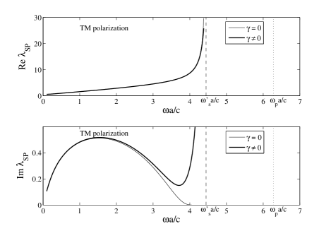
Figure 7: Regge trajectory for the SP Regge pole: comparison between a non-absorbing and an absorbing sphere. $\epsilon_{c}(\omega)$ has the Drude type behavior with $\epsilon_{\infty}=1$ and $\omega_{p}a/c=2\pi$ while $\epsilon_{h}=1$. As $\omega a/c\to\omega^{\prime}_{s}a/c$, the real part of the SP Regge pole always increases indefinitely while its imaginary part vanishes for $\gamma=0$ and increases indefinitely for $\gamma\not=0$.

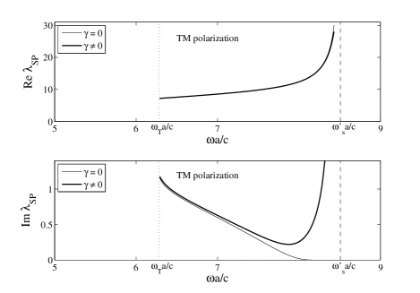
Figure 8: Regge trajectory for the SP Regge pole: comparison between a non-absorbing and an absorbing sphere. $\epsilon_{c}(\omega)$ has the ionic crystal behavior with $\epsilon_{\infty}=2$, $\omega_{T}a/c=2\pi$ and $\omega_{L}a/c=3\pi$ while $\epsilon_{h}=1$. As $\omega a/c\to\omega^{\prime}_{s}a/c$, the real part of the SP Regge pole increases indefinitely while its imaginary part vanishes for $\gamma=0$ and increases indefinitely for $\gamma\not=0$.

In Figs. 7 and 8, we have displayed the Regge trajectories of the SP for the two configurations previously studied. Absorption does not modify the global behavior of the real part of the SP Regge pole. It should be also noted that, as $\omega\to\omega^{\prime}_{s}$, this real part increases indefinitely. By contrast, absorption increases significantly the imaginary part of the Regge trajectory of the SP: for the non-absorbing sphere, this imaginary part vanishes as $\omega\to\omega^{\prime}_{s}$ while, for the absorbing sphere, it first exhibits a minimum and then increases indefinitely as $\omega\to\omega^{\prime}_{s}$. In other words, absorption has a strong influence on the damping of the SP but does not modify its dispersion relation. For other configurations (i.e., for other values of the parameters $\epsilon_{\infty}$, $\epsilon_{h}$, $\omega_{p}$, $\omega_{T}$, $\omega_{L}$ and $\gamma$), the SP Regge pole behavior is very similar. The minimum of the imaginary part of the Regge trajectory always exists (for the absorbing sphere). This feature could be interesting with in mind practical applications using real materials.

Table 1: The first complex frequencies of RSPM’s (TM polarization). $\epsilon_{c}(\omega)$ has the Drude type behavior with $\epsilon_{\infty}=1$, $\omega_{p}a/c=2\pi$ and $\gamma=0$ while $\epsilon_{h}=1$.

	Exact	Exact	Semiclassical	Semiclassical
$\ell$	$(\omega^{(0)}_{\ell{\mathrm{SP}}})a/c$	$(\Gamma_{\ell{\mathrm{SP}}}/2)a/c$	$(\omega^{(0)}_{\ell{\mathrm{SP}}})a/c$	$(\Gamma_{\ell{\mathrm{SP}}}/2)a/c$
1	0.897849	0.407409	0.944599	0.381875
2	1.762396	0.391747	1.734451	0.380517
3	2.475717	0.268405	2.430280	0.267887
4	3.019638	0.136587	2.992907	0.138470
5	3.412422	0.049796	3.404834	0.050338
6	3.683304	0.012179	3.682351	0.012207
7	3.862800	0.001935	3.862752	0.001934
8	3.982206	0.000209	3.982204	0.000208
9	4.065198	0.000016	4.065196	0.000016
10	4.125633	0.000001	4.125631	0.000001

Table 2: The first complex frequencies of RSPM’s (TM polarization). $\epsilon_{c}(\omega)$ has the Drude type behavior with $\epsilon_{\infty}=1$, $\omega_{p}a/c=2\pi$ and $\gamma=1/100$ while $\epsilon_{h}=1$.

	Exact	Exact	Semiclassical	Semiclassical
$\ell$	$(\omega^{(0)}_{\ell{\mathrm{SP}}})a/c$	$(\Gamma_{\ell{\mathrm{SP}}}/2)a/c$	$(\omega^{(0)}_{\ell{\mathrm{SP}}})a/c$	$(\Gamma_{\ell{\mathrm{SP}}}/2)a/c$
1	0.894546	0.408326	0.942572	0.382753
2	1.757428	0.395822	1.731152	0.384335
3	2.470440	0.276889	2.426006	0.276611
4	3.015603	0.149847	2.988477	0.152411
5	3.410258	0.067443	3.401552	0.068144
6	3.682529	0.033581	3.681107	0.033585
7	3.862589	0.026173	3.863243	0.026087
8	3.982111	0.026321	3.983622	0.026089
9	4.065111	0.027345	4.067129	0.027396
10	4.125541	0.028160	4.128020	0.028289

Tables 1, 2, 3 and 4 present samples of complex frequencies of RSPM’s for the two configurations previously considered. They are calculated from the semiclassical formulas (25) and (26) by using the Regge trajectories numerically determined by solving (17) (see Figs. 7 and 8). We can observe a very good agreement between the “exact” and the semiclassical spectra for “high” frequencies as well as a rather good agreement for “low” frequencies. Furthermore, from the behavior of Regge trajectories near the limiting frequencies $\omega^{\prime}_{s}$ and the semiclassical formulas (25) and (26), we easily obtain the existence of the families of resonances close to the real axis of the complex $\omega$-plane which converge, for large $\ell$, to the limiting frequency $\omega^{\prime}_{s}+i\omega^{\prime\prime}_{s}$. In conclusion, we have established a connection between the complex frequencies of RSPM’s and a particular surface wave, the so-called SP, described by a particular Regge pole of the electric part of the $S$ matrix and which orbits around the sphere.

We conclude this section by making a brief comparison with the results obtained in our previous study concerning metallic and semiconducting cylindersAncey et al. (2004). Of course, such a comparison can be achieved only in the non-absorbing case. From Regge trajectories (see Figs. 6 and 7 of Ref. Ancey et al., 2004 and Figs. 7 and 8 of the present article), we can observe that the behavior of the SP orbiting around a metallic/semiconducting sphere is, at first sight, rather similar to the behavior of the SP orbiting around a metallic/semiconducting cylinder, even if they correspond to different polarizations (TE polarization for the cylinder and TM polarization for the sphere). In fact, as we shall see in the next section, in the absence of absorption the transition from two dimensions to three dimensions induces some curvature corrections on the wave numbers $k_{\mathrm{SP}}(\omega)$ of the SP’s and the behaviors are identical only in the radius limit $a\to\infty$, i.e., in the flat interface limit. In the presence of absorption, we shall prove than a supplementary correction associated with the imaginary part of the complex dielectric constant is necessary in order to interpret the behavior observed in Figs. 7 and 8.

Table 3: Some complex frequencies of RSPM’s (TM polarization). $\epsilon_{c}(\omega)$ has the ionic crystal behavior with $\epsilon_{\infty}=2$, $\omega_{T}a/c=2\pi$, $\omega_{L}a/c=3\pi$ and $\gamma=0$ while $\epsilon_{h}=1$.

	Exact	Exact	Semiclassical	Semiclassical
$\ell$	$(\omega^{(0)}_{\ell{\mathrm{SP}}})a/c$	$(\Gamma_{\ell{\mathrm{SP}}}/2)a/c$	$(\omega^{(0)}_{\ell{\mathrm{SP}}})a/c$	$(\Gamma_{\ell{\mathrm{SP}}}/2)a/c$
9	7.436965	0.111396	7.405909	0.115670
10	7.700893	0.037894	7.694243	0.038461
11	7.887534	0.009632	7.886710	0.009713
12	8.015334	0.001839	8.015239	0.001844
13	8.104140	0.000274	8.104087	0.000273
14	8.168509	0.000034	8.168477	0.000034
15	8.217128	0.000005	8.217069	0.000003
16	8.255038	0.000002	8.254956	0.000000
17	8.285324	0.000001	8.285231	0.000000

Table 4: Some complex frequencies of RSPM’s (TM polarization). $\epsilon_{c}(\omega)$ has the ionic crystal behavior with $\epsilon_{\infty}=2$, $\omega_{T}a/c=2\pi$, $\omega_{L}a/c=3\pi$ and $\gamma=1/100$ while $\epsilon_{h}=1$.

	Exact	Exact	Semiclassical	Semiclassical
$\ell$	$(\omega^{(0)}_{\ell{\mathrm{SP}}})a/c$	$(\Gamma_{\ell{\mathrm{SP}}}/2)a/c$	$(\omega^{(0)}_{\ell{\mathrm{SP}}})a/c$	$(\Gamma_{\ell{\mathrm{SP}}}/2)a/c$
9	7.433460	0.131422	7.399537	0.137680
10	7.699297	0.060583	7.690606	0.061609
11	7.887001	0.034650	7.885688	0.035096
12	8.015186	0.028573	8.016067	0.028737
13	8.104082	0.028141	8.105881	0.028098
14	8.168462	0.028649	8.170808	0.027735
15	8.217080	0.029138	8.219861	0.029527
16	8.254988	0.029514	8.258154	0.029563
17	8.285273	0.029801	8.288906	0.029931

IV Semiclassical analysis: Asymptotics for the SP and physical description

An analytical expression for the Regge pole $\lambda_{\mathrm{SP}}$ and therefore a deeper physical understanding of the SP behavior can be obtained by solving Eq. (17) for $\lambda=\lambda_{\mathrm{SP}}$. For the TM polarization, Eq. (17) reduces to [see Eq. (9b)]

$$\frac{\sqrt{\epsilon_{c}(\omega)}}{\sqrt{\epsilon_{h}}}\frac{\zeta_{\lambda_{\mathrm{SP}}-1/2}^{(1)^{\prime}}\left(\sqrt{\epsilon_{h}}a\omega/c\right)}{\zeta_{\lambda_{\mathrm{SP}}-1/2}^{(1)}\left(\sqrt{\epsilon_{h}}a\omega/c\right)}=\frac{\psi_{\lambda_{\mathrm{SP}}-1/2}^{\prime}\left(\sqrt{\epsilon_{c}(\omega)}a\omega/c\right)}{\psi_{\lambda_{\mathrm{SP}}-1/2}\left(\sqrt{\epsilon_{c}(\omega)}a\omega/c\right)}.$$ (28)

This equation cannot be solved exactly but only perturbatively. With this aim in view, we must first replace Ricatti-Bessel functions by spherical Bessel functions. We then use their relations with the ordinary Bessel functions (see Ref. Abramowitz and Stegun, 1965)

$$j_{\lambda}(z)=\sqrt{\frac{\pi}{2z}}J_{\lambda+1/2}(z)\quad\mathrm{and}\quad h^{(1)}_{\lambda}(z)=\sqrt{\frac{\pi}{2z}}H^{(1)}_{\lambda+1/2}(z)$$ (29)

and we finally replace the Bessel function $J_{\lambda}(z)$ by the modified Bessel function $I_{\lambda}(z)$ (see Ref. Abramowitz and Stegun, 1965) in order to take into account the fact that $\mathrm{Re}\,\epsilon_{c}(\omega)<0$. Eq. (28) then reduces to

$$\frac{1}{\sqrt{\epsilon_{h}}}\frac{H_{\lambda_{\mathrm{SP}}}^{(1)^{\prime}}(\sqrt{\epsilon_{h}}\omega a/c)}{H_{\lambda_{\mathrm{SP}}}^{(1)}(\sqrt{\epsilon_{h}}\omega a/c)}+\frac{1}{2\epsilon_{h}}\left(\frac{c}{\omega a}\right)$$

$$\quad=-\frac{1}{\sqrt{-\epsilon_{c}(\omega)}}\frac{I^{\prime}_{\lambda_{\mathrm{SP}}}(\sqrt{-\epsilon_{c}(\omega)}\omega a/c)}{I_{\lambda_{\mathrm{SP}}}(\sqrt{-\epsilon_{c}(\omega)}\omega a/c)}+\frac{1}{2\epsilon_{c}(\omega)}\left(\frac{c}{\omega a}\right).$$

This equation must be compared with Eq. (26) of Ref. Ancey et al., 2004 which provides the SP Regge pole for the cylinder. The first term on the left-hand side and the right-hand side of Eq. (IV) are exactly those appearing in Eq. (26) of Ref. Ancey et al., 2004. The two others terms are simple curvature corrections due to the change of dimension. As a consequence, Eq. (IV) can be solved following the method used in order to solve Eq. (26) of Ref. Ancey et al., 2004 but, now, it is important to take carefully into account the fact that the dielectric function $\epsilon_{c}(\omega)$ has an imaginary part [see Eqs. (5b) and (6b)]. It should be noted that the existence of such curvature corrections has been first observed by BerryBerry (1975) in the restricted case of non-dispersive and non-absorbing spheres.

On the right-hand side of (IV), by assuming $|\lambda_{\mathrm{SP}}|\gg|\sqrt{-\epsilon_{c}(\omega)}\omega a/c|$, we can writeAbramowitz and Stegun (1965); Ancey et al. (2004)

$$-\frac{1}{\sqrt{-\epsilon_{c}(\omega)}}\frac{I^{\prime}_{\lambda_{\mathrm{SP}}}(\sqrt{-\epsilon_{c}(\omega)}\omega a/c)}{I_{\lambda_{\mathrm{SP}}}(\sqrt{-\epsilon_{c}(\omega)}\omega a/c)}$$

$$\qquad\qquad\qquad\sim\frac{\left[\lambda_{\mathrm{SP}}^{2}-\epsilon_{c}(\omega)(\omega a/c)^{2}\right]^{1/2}}{\epsilon_{c}(\omega)(\omega a/c)}.$$ (31)

On the left-hand side of (IV), by assuming $|\lambda_{\mathrm{SP}}|\gg\sqrt{\epsilon_{h}}\omega a/c$, we can writeWatson (1995); Nussenzveig (1965); Ancey et al. (2004)

$$\frac{1}{\sqrt{\epsilon_{h}}}\frac{H_{\lambda_{\mathrm{SP}}}^{(1)^{\prime}}(\sqrt{\epsilon_{h}}\omega a/c)}{H_{\lambda_{\mathrm{SP}}}^{(1)}(\sqrt{\epsilon_{h}}\omega a/c)}$$

$$\qquad\sim-\frac{\left[\lambda_{\mathrm{SP}}^{2}-\epsilon_{h}(\omega a/c)^{2}\right]^{1/2}}{\epsilon_{h}(\omega a/c)}$$

$$\qquad\quad\times\left(1-i\,e^{2\alpha(\lambda_{\mathrm{SP}},\sqrt{\epsilon_{h}}\omega a/c)}\right)$$ (32)

where

$$\alpha(\lambda,z)=(\lambda^{2}-z^{2})^{1/2}-\lambda\ln\left(\frac{\lambda+(\lambda^{2}-z^{2})^{1/2}}{z}\right).$$ (33)

It should be noted that in Eq. (IV) we have taken into account an exponentially small contribution (the term $\exp{[2\alpha(\lambda_{\mathrm{SP}},\sqrt{\epsilon_{h}}\omega a/c)]}$) which lies beyond all orders in perturbation theory. This term can be captured by carefully taking into account Stokes phenomenon Berry (1989); Dingle (1973); Segur et al. (1991); Berry and Howls (1990) and is necessary to extract the asymptotic expression of the imaginary part of $\lambda_{\mathrm{SP}}$. (In Eq. (IV) we have given to the Stokes multiplier function the value $1/2$.) For more precision, we refer to our previous articleAncey et al. (2004).

By using (IV) and (IV) as well as $|\epsilon^{\prime\prime}_{c}(\omega)|\ll|\epsilon^{\prime}_{c}(\omega)|$, Eq. (IV) can be solved perturbatively and we find

$$\mathrm{Re}\,\lambda_{\mathrm{SP}}(\omega)\sim\left(\frac{\omega a}{c}\right)\sqrt{\frac{\epsilon_{h}\epsilon^{\prime}_{c}(\omega)}{\epsilon_{h}+\epsilon^{\prime}_{c}(\omega)}}\left(1+\frac{1}{2\sqrt{-[\epsilon_{h}+\epsilon^{\prime}_{c}(\omega)]}}\left(\frac{c}{\omega a}\right)\right),$$ (34a)

and

$$\mathrm{Im}\,\lambda_{\mathrm{SP}}(\omega)=\mathrm{Im}_{1}\,\lambda_{\mathrm{SP}}(\omega)+\mathrm{Im}_{2}\,\lambda_{\mathrm{SP}}(\omega)$$ (34b)

with

$$\mathrm{Im}_{1}\,\lambda_{\mathrm{SP}}(\omega)\sim\left[\frac{{\epsilon^{\prime}_{c}}^{2}(\omega)}{{\epsilon^{\prime}_{c}}^{2}(\omega)-\epsilon_{h}^{2}}\right]\frac{\left[\mathrm{Re}\,\lambda_{\mathrm{SP}}(\omega)\right]^{2}-\epsilon_{h}\left({\omega a/c}\right)^{2}}{\mathrm{Re}\,\lambda_{\mathrm{SP}}(\omega)}\left[1-\frac{\epsilon_{h}/\epsilon^{\prime}_{c}(\omega)}{2\sqrt{-[\epsilon_{h}+\epsilon^{\prime}_{c}(\omega)]}}\left(\frac{c}{\omega a}\right)\right]\exp\{{2\alpha[\mathrm{Re}\,\lambda_{\mathrm{SP}}(\omega),\sqrt{\epsilon_{h}}\omega a/c]\}},$$

(34c)

$$\mathrm{Im}_{2}\,\lambda_{\mathrm{SP}}(\omega)\sim\left(\frac{\omega a}{c}\right)\sqrt{\frac{\epsilon_{h}\epsilon^{\prime}_{c}(\omega)}{\epsilon_{h}+\epsilon^{\prime}_{c}(\omega)}}\frac{\epsilon_{h}\epsilon^{\prime\prime}_{c}(\omega)}{2\epsilon^{\prime}_{c}(\omega)[\epsilon_{h}+\epsilon^{\prime}_{c}(\omega)]}\left[1+\frac{1}{2\sqrt{-[\epsilon_{h}+\epsilon^{\prime}_{c}(\omega)]}}\left(\frac{c}{\omega a}\right)\right].$$ (34d)

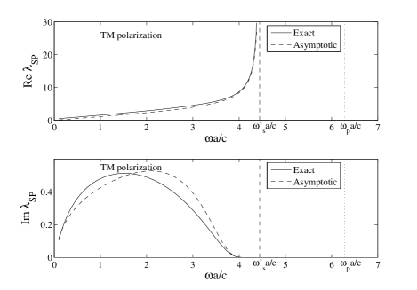
Figure 9: Regge trajectory for the SP Regge pole. Comparison between exact and asymptotic theories. $\epsilon_{c}(\omega)$ has the Drude type behavior with $\epsilon_{\infty}=1$, $\omega_{p}a/c=2\pi$ and $\gamma=0$ while $\epsilon_{h}=1$.

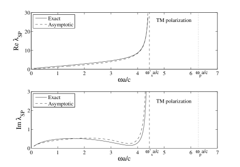
Figure 10: Regge trajectory for the SP Regge pole. Comparison between exact and asymptotic theories. $\epsilon_{c}(\omega)$ has the Drude type behavior with $\epsilon_{\infty}=1$, $\omega_{p}a/c=2\pi$ and $\gamma=1/100$ while $\epsilon_{h}=1$.

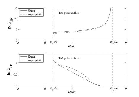
Figure 11: Regge trajectory for the SP Regge pole. Comparison between exact and asymptotic theories. $\epsilon_{c}(\omega)$ has the ionic crystal behavior with $\epsilon_{\infty}=2$, $\omega_{T}a/c=2\pi$, $\omega_{L}a/c=3\pi$ and $\gamma=0$ while $\epsilon_{h}=1$.

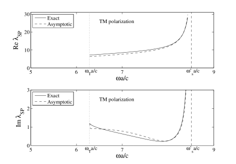
Figure 12: Regge trajectory for the SP Regge pole. Comparison between exact and asymptotic theories. $\epsilon_{c}(\omega)$ has the ionic crystal behavior with $\epsilon_{\infty}=2$, $\omega_{T}a/c=2\pi$, $\omega_{L}a/c=3\pi$ and $\gamma=1/100$ while $\epsilon_{h}=1$.

Equations (34a), (34b), (34c) and (34d) provide analytic expressions for the dispersion relation and the damping of the SP. The following important features must be noted:

– The SP only exists in the frequency range where $\epsilon_{h}+\epsilon^{\prime}_{c}(\omega)<0$. Its dispersion relation [see Eqs. (34a) and (23)] only depends on the real part of the dielectric function: thus, it is slightly modify by absorption. Its attenuation [see Eqs. (34b), (34c) and (34d)] is compounded by two contributions. The first one [see Eq. (34c] only depends on the real part of the dielectric function and presents an exponentially small attenuation. It fully describes the attenuation of the SP propagating on a non-absorbing sphere. The second contribution [see Eq. (34d] is proportional to the imaginary part of the dielectric function and is therefore directly linked to absorption. It increases indefinitely as $\omega\to\omega^{\prime}_{s}$ and semiclassically explains the behavior already described in Sec. III.

– The wave number $k_{\mathrm{SP}}(\omega)$ associated with the SP is obtained from (34a) and (23) and is given by

$$k_{\mathrm{SP}}(\omega)\sim\left(\frac{\omega}{c}\right)\sqrt{\frac{\epsilon_{h}\epsilon^{\prime}_{c}(\omega)}{\epsilon_{h}+\epsilon_{c}(\omega)}}$$

$$\qquad\times\left[1+\frac{1}{2\sqrt{-[\epsilon_{h}+\epsilon^{\prime}_{c}(\omega)]}}\left(\frac{c}{\omega a}\right)\right].$$ (35)

This relation could permit us to derive analytically the phase velocity $v_{p}=\omega/k_{\mathrm{SP}}(\omega)$ as well as the group velocity $v_{g}=d\omega/dk_{\mathrm{SP}}(\omega)$ of the SP [see also Eq.  (24)].

– For $a\to\infty$ – i.e., in the flat interface limit – we recover the usual dispersion relation of a SP supported by a flat metal-dielectric or semiconductor-dielectric interface (see, for example, Ref. Raether, 1988).

– The imaginary part (34c) of $\lambda_{\mathrm{SP}}$ vanishes for $a\to\infty$: the SP supported by the flat interface between an ordinary dielectric and a non-absorbing metallic or semiconducting medium has no damping (see, for example, Ref. Raether, 1988).

– By inserting the expression (34a) for $\lambda_{\mathrm{SP}}(\omega)$ into the Bohr-Sommerfeld quantization condition (25), we obtain an eighth-order polynomial equation which can be solved numerically and which provides rather precisely the resonance excitation frequencies $\omega^{(0)}_{\ell{\mathrm{SP}}}$.

– We have numerically tested the formulas (34a), (34b), (34c) and (34d) for various values of the parameters $\epsilon_{\infty}$, $\epsilon_{h}$, $\omega_{p}$, $\omega_{T}$, $\omega_{L}$ and $\gamma$. In all cases, they provide rather good approximations for $\mathrm{Re}~{}\lambda_{\mathrm{SP}}$ and $\mathrm{Im}~{}\lambda_{\mathrm{SP}}$ (see Figs. 9, 10, 11 and 12 for the two configurations previously studied).

The connection with the results obtained in our previous study concerning metallic and semiconducting cylindersAncey et al. (2004) can be made. The transition from the cylinder to the sphere induces some curvature corrections on the real and imaginary parts of the Regge pole of the SP [the second term on the right-hand side of (34a), the third term on the right-hand side of (34c) and the fourth term on the right-hand side of (34d)] which come from the second terms on the left-hand side and the right-hand side of Eq. (IV). Without the curvature corrections, Eqs. (34a), (34b), (34c) and (34d) reduce to

$$\mathrm{Re}\,\lambda_{\mathrm{SP}}(\omega)\sim\left(\frac{\omega a}{c}\right)\sqrt{\frac{\epsilon_{h}\epsilon^{\prime}_{c}(\omega)}{\epsilon_{h}+\epsilon^{\prime}_{c}(\omega)}},$$ (36a)

and

$$\mathrm{Im}\,\lambda_{\mathrm{SP}}(\omega)=\mathrm{Im}_{1}\,\lambda_{\mathrm{SP}}(\omega)+\mathrm{Im}_{2}\,\lambda_{\mathrm{SP}}(\omega)$$ (36b)

with

$$\mathrm{Im}_{1}\,\lambda_{\mathrm{SP}}(\omega)\sim\left[\frac{{\epsilon^{\prime}_{c}}^{2}(\omega)}{{\epsilon^{\prime}_{c}}^{2}(\omega)-\epsilon_{h}^{2}}\right]$$

$$\qquad\qquad\times\frac{\left[\mathrm{Re}\,\lambda_{\mathrm{SP}}(\omega)\right]^{2}-\epsilon_{h}\left({\omega a/c}\right)^{2}}{\mathrm{Re}\,\lambda_{\mathrm{SP}}(\omega)}$$

$$\qquad\qquad\times\exp\{{2\alpha[\mathrm{Re}\,\lambda_{\mathrm{SP}}(\omega),\sqrt{\epsilon_{h}}\omega a/c]\}},$$ (36c)

$$\mathrm{Im}_{2}\,\lambda_{\mathrm{SP}}(\omega)\sim\left(\frac{\omega a}{c}\right)\sqrt{\frac{\epsilon_{h}\epsilon^{\prime}_{c}(\omega)}{\epsilon_{h}+\epsilon^{\prime}_{c}(\omega)}}\frac{\epsilon_{h}\epsilon^{\prime\prime}_{c}(\omega)}{2\epsilon^{\prime}_{c}(\omega)[\epsilon_{h}+\epsilon^{\prime}_{c}(\omega)]}.$$

(36d)

These last expressions are the semiclassical formulas providing the dispersion relation and the damping of the SP propagating on the cylinder in the non-absorbing and absorbing cases. They are much more general that the corresponding formulas obtained in our previous paperAncey et al. (2004). Indeed, Eq. (36a) has been already obtained in Ref. Ancey et al., 2004 in the restricted context of the non-absorbing cylinder [see Eq. (40a)] and, in the same way, Eq. (36c) has been obtained in a less practical form [see Eq. (40b) in Ref. Ancey et al., 2004].

V Conclusion and perspectives

In this article, we have introduced the CAM method in order (i) to study the interaction of electromagnetic waves with non-absorbing or absorbing metallic and semiconducting spheres and (ii) to completely describe the resonant aspects of this problem. This allows us to provide a physical explanation for the excitation mechanism of RSPM’s as well as a simple mathematical description of the surface wave (i.e., the SP) that generates them. It should be noted that our approach is not limited to the metals and semiconductors described by (2) and (3) but remains still valid for more general materials (see the conclusion of Ref. Ancey et al., 2004).

In Ref. Ancey et al., 2004, we have developed a new picture of the photon-cylinder system (see also the analysis of the works of Ito and Sakoda Ito and Sakoda (2001); Sakoda (2001) in the conclusion of Ref. Ancey et al., 2004): it can be viewed as an artificial atom for which the photon plays the role of an electron. Mutatis mutandis, this picture is still valid for the photon-sphere system: RSPM’s are long-lived quasibound states for this atom, the associated complex frequencies are Breit-Wigner-type resonances while the trajectory of the SP which generates them and which is supported by the sphere surface is a Bohr-Sommerfeld-type orbit. Recently, Guzatov and Klimov Guzatov and Klimov (arXiv:physics/0703251) have also developed the analogy between a metallic sphere and an ordinary atom and, more generally, between a cluster of metallic spheres and ordinary molecules, introducing on that occasion the terms “plasmonic atom” and “plasmonic molecules”. It should be noted that their approach uses the quasi-static approximation for the description of the electromagnetic field. As a consequence, they have found that the “energy levels” of the photon-sphere system are real (bound states). In fact, as we have shown, the imaginary parts of the “energy levels” do not vanish (quasi-bound states): they correspond to exponentially small terms lying beyond all orders in perturbation theory.

Our results could be useful (i) in the context of three-dimensional photonic crystal physics (the existence of dispersionless band for the arrays of metallic or semiconducting spheres is associated with the excitation of the sphere RPSM’s), (ii) in cavity quantum electrodynamics and, more generally, (iii) in the context of nanotechnologies and plasmonics. Here, we shall more particularly focus our discussion to the possible applications to the Casimir effect.

Since the precise experiments carried out by Lamoreaux Lamoreaux (1997) in 1997, it is necessary to completely describe, from a theoretical point of view, the Casimir interaction between two metallic spheres or between a metallic sphere and a plane (for a review on recent experiments and problematic, we refer to Ref. Bordag et al., 2001). A semiclassical description of this interaction could be achieved by extending to electrodynamics the Korringa-Kohn-Rostoker (KKR) type method developed in Ref. Bulgac et al., 2006 for the scalar Casimir effect. Because at short distance RSPM’s provide the dominant contribution to the Casmir interaction Genet et al. (2004); Henkel et al. (2004), it would be then necessary to carefully take into account the contributions of all the periodic orbits associated with the SP. In this context, the description that we gave in Sec. IV could be helpful.