Gravitational instability of a dilute fully ionized gas in the presence of the Dufour effect

Abstract

The gravitational instability of a fully ionized gas is analyzed within the framework of linear irreversible thermodynamics. In particular, the presence of a heat flux corresponding to generalized thermodynamic forces is shown to affect the properties of the dispersion relation governing the stability of this kind of system in certain problems of interest.

I Introduction

The study of transport processes in plasmas leads directly to a set of partial differential equations that describes the evolution of the local thermodynamic variables relevant to its physical description. Linear irreversible thermodynamics predicts the coupling of all thermodynamic fluxes and forces involving all possible tensors of the same rank key-1 . In this context, for multicomponent systems, the problem of gravitational instability in the presence of a heat flux associated to a density gradient (Dufour effect) is ought to be examined in order to address its implications regarding the Jeans instability criterion. The reciprocal effect, a mass flux due to a temperature gradient (Soret effect), does not affect the continuity equation for the total density of the system, and therefore does not alter the Jeans instability criterion.

While lots of results regarding the effect of dissipation on the Jeans criterion have been obtained in several works key-2 , to the authors’ knowledge, this is the first time in which the Dufour effect is taken into account in calculations regarding gravitational stability. The numerical values for the transport coefficients used in this work have been recently obtained by the authors based on the Chapman-Enskog expansion used in order to solve Boltzmann’s equation key-3 key-4 . Similar results have been obtained in terms of several formalisms, from the works done by Spitzer key-5 , Braginski key-6 , Marshall key-7 and Balescu key-8 .

The structure of this work is as follows. In section 2, the basic hydrodynamic equations are presented including the Dufour flux for a binary mixture of dilute gases. In section 3 the linearized system of equations for the fluctuations in the local density $\delta\rho$, the local temperature $\delta T$ and the hydrodynamic velocity $\delta\vec{u}$ are obtained together with the corresponding dispersion relation associated to it. Section 4 is devoted to the study of the explicit gravitational stability criterion for the binary plasma. The last section of this work is dedicated to a discussion of the results, addressing the conditions in which the various thermodynamic forces turn out to be relevant in the study of gravitational stability.

II Basic equations and transport coefficients

Consider a fully ionized system formed by species $i=1,\,2$, $\rho_{1}$ standing for the electron mass density and $\rho_{2}$, corresponding for the ion mass density. The task to accomplish is to determine the importance of the various dissipative effects on Jeans instability. Total mass conservation reads:

$$\frac{\partial\rho}{\partial t}+\nabla\cdot\left(\rho\vec{u}\right)=0$$ (1)

In Eq. (1) $\vec{u}$ corresponds to the hydrodynamic velocity of the mixture defined by the relation

$$\left(\rho_{1}+\rho_{2}\right)\vec{u}=\rho\vec{u}=\rho_{1}\vec{u}_{1}+\rho_{2}\vec{u_{2}}.$$ (2)

The total density of the mixture is given by $\rho=\rho_{1}+\rho_{2}$. For a quasi-neutral plasma, the number densities are $n_{1}=n_{2}=\frac{n}{2}$, where $\rho_{i}=m_{i}n_{i}$ and $n=n_{1}+n_{2}$, $m_{1}$and $m_{2}$ being the electron and proton masses, respectively. Also, $\vec{u}_{i}$ represents the average velocity corresponding to species $i$.

The balance equation for linear momentum reads key-1 :

$$\frac{\partial\left(\rho\vec{u}\right)}{\partial t}+\nabla p+\nabla\cdot\left(\rho\vec{u}\vec{u}+\tau^{kl}\right)=-\rho\nabla\varphi$$ (3)

In Eq. (3), $p$ represents the local pressure of the fluid , $\tau^{kl}$ is the viscous contribution to the stress tensor and $\varphi$ is the gravitational potential which, in Newtonian mechanics, satisfies the Poisson equation

$$\nabla^{2}\varphi=-4\pi G\rho$$ (4)

Total energy conservation leads to a well known expression for the evolution of the local temperature of the system $T$, namely key-1 ,

$$\rho c_{v}\frac{\partial T}{\partial t}-\left(\frac{\partial\varepsilon}{\partial\rho}\right)_{T}\rho^{2}\nabla\cdot\vec{u}=-\nabla\cdot\left(\vec{J}_{[Q]}\right)-\rho c_{v}\vec{u}\cdot\nabla T-p\nabla\cdot\vec{u}$$ (5)

where $\rho\varepsilon$ is the internal local energy density. The heat flux vector $\vec{J}_{[Q]}$ in Eq. (5) contains a contribution due to a temperature gradient (Fourier law) and a contribution associated to a density gradient (Dufour effect):

$$\vec{J}_{[Q]}=-\kappa\nabla T-\frac{\mathcal{D}}{2T}\nabla T-\frac{\mathcal{D}}{2\rho}\nabla\rho$$ (6)

where $\kappa$ stands for the heat conductivity and $\mathcal{D}$ is the Dufour coefficient. Equations (1), (3) and (5), together with their corresponding constitutive equations relating thermodynamic fluxes and forces, form a complete set of non-linear partial differential equations which is in general difficult to work with. Nevertheless, stability analysis around constant equilibrium values may be readily performed by standard methods. This will be the subject of the next section.

III Linearized transport equations

A first order perturbative stability analysis can be performed assuming that any local thermodynamic variable $X$ in this system has a constant average value $\left\langle X\right\rangle$ and a fluctuation around it $\delta X$, so that

$$X=\left\langle X\right\rangle+\delta X$$ (7)

We can now rewrite the system given by Eqs. (1), (3) and (5) in terms of the fluctuations. For simplicity, $\left\langle\vec{u}\right\rangle=\vec{0}$ is assumed. The linearized continuity equation becomes:

$$\frac{\partial\left(\delta\rho\right)}{\partial t}+\left\langle\rho\right\rangle\delta\theta=0$$ (8)

where $\delta\theta\equiv\nabla\cdot\delta\vec{u}$. Following the usual approach, the stress tensor in Eq. (3) is coupled linearly to the traceless symmetric part of the velocity gradient through shear viscosity. Thus, the linearized momentum balance equation becomes:

$$\left\langle\rho\right\rangle\frac{\partial\left(\delta\theta\right)}{\partial t}+\frac{3}{5}C_{s}^{2}\nabla^{2}\left(\delta\rho\right)+\left\langle\rho\right\rangle\frac{3C_{s}^{2}}{5T}\nabla^{2}\left(\delta T\right)-D_{v}\nabla^{2}\left(\delta\theta\right)=-4\pi G\left\langle\rho\right\rangle\delta\rho$$ (9)

where $D_{v}$ =$\frac{4}{3}\eta$, $\eta$ standing for the shear viscosity measured in international units ($Pa-sec$). In our dilute (ideal) plasma, bulk viscosity is neglected. We have also used the fact that, for an ideal gas, $\nabla p=\frac{1}{\gamma}C_{s}^{2}\nabla\rho+\frac{C_{s}^{2}}{\gamma T}\nabla T$ where $C_{s}$ is the adiabatic speed of sound and $\gamma$ is the heat capacities ratio ($\gamma=5/3$). Therefore, the linearized energy balance equation is written as:

$$\frac{\partial\left(\delta T\right)}{\partial t}-\frac{1}{\left\langle\rho\right\rangle c_{v}}\left(\kappa+\frac{\mathcal{D}}{2\left\langle T\right\rangle}\right)\nabla^{2}\delta T-\frac{1}{\left\langle\rho\right\rangle^{2}c_{v}}\frac{\mathcal{D}}{2}\nabla^{2}\delta\rho+\frac{2\left\langle T\right\rangle}{3}\delta\theta=0$$ (10)

Notice that the Dufour coefficient $\mathcal{D}$ vanishes for a simple fluid key-7 ; key-8 , but in principle affects the energy balance in the binary mixture. For our ideal gas, $c_{v}=\frac{3k}{2m_{2}}$ is the heat capacity measured in $\frac{J}{KgK}$, $k=1.38\times 10^{-23}\frac{J}{K}$. $\kappa$ is measured in $\frac{J}{Kms}$ and $\mathcal{D}$ is given in $\frac{J}{ms}$. The values of these coefficients for a dilute plasma have been obtained from plasma kinetic theory key-4 ; key-8 . They can be written as:

$$\kappa=\frac{5}{4}\frac{\left\langle n\right\rangle k^{2}\left\langle T\right\rangle}{m_{1}}\left(2.01\tau\right)$$ (11)

$$\mathcal{D}=\frac{5}{2}\frac{\left\langle n\right\rangle\left(k\left\langle T\right\rangle\right)^{2}}{m_{1}}\left(0.29\tau\right)$$ (12)

Here $\tau$ is a characteristic time given by

$$\tau=\frac{4\left(2\pi\right)^{3/2}\sqrt{m_{1}}\epsilon_{0}^{2}\left(kT\right)^{3/2}}{ne^{4}\psi}$$

where $e$ is the electron charge, $\epsilon_{0}$ is he dielectric constant and $\psi$ is the usual Coulomb logarithm key-5 . The shear viscosity coefficient $\eta$ is estimated by using the Eucken number for an ideal gas, $5/2=\kappa/\eta c_{v}$. We are now in position to address the importance of dissipation, including the Dufour effect, on the Jeans instability by means of the analysis of the corresponding dispersion relation. In order to derive the desired stability criterion, we perform a Laplace transform in time and a Fourier transform in space to the system (8-10). The corresponding equations become

$$s\delta\tilde{\hat{\rho}}+\left\langle\rho\right\rangle\delta\tilde{\hat{\theta}}=\delta\hat{\rho}\left(\vec{q},0\right)$$ (13)

$$\left(4\pi G\left\langle\rho\right\rangle-\frac{3}{5}C_{s}^{2}q^{2}\right)\delta\tilde{\hat{\rho}}+\left(D_{v}q^{2}+\left\langle\rho\right\rangle s\right)\delta\tilde{\hat{\theta}}-\frac{3\left\langle\rho\right\rangle C_{s}^{2}}{5\left\langle T\right\rangle}q^{2}\delta T=\left\langle\rho\right\rangle\delta\hat{\theta}\left(\vec{q},\,0\right)$$ (14)

$$\frac{\mathcal{D}}{2\left\langle\rho\right\rangle^{2}c_{v}}q^{2}\tilde{\hat{\rho}}+\frac{2\left\langle T\right\rangle}{3}\delta\tilde{\hat{\theta}}+\left[s+\frac{1}{\left\langle\rho\right\rangle c_{v}}\left(\kappa+\frac{\mathcal{D}}{2\left\langle T\right\rangle}\right)q^{2}\right]\delta\tilde{\hat{T}}=\delta\hat{T}\left(\vec{q},\,0\right)$$ (15)

Here, the symbol $\tilde{\hat{X}}=\tilde{\hat{X}}\left(\vec{q},\,s\right)$ stands for the successive Laplace-Fourier transforms of the thermodynamic variable $X$. The wave vector is denoted by $\vec{q}$ and the corresponding Laplace frequency is $s$.

It is interesting to notice that the first term in Eq. (15) has never been taken into account in the study of the Jeans instability. The term vanishes in a single component system and may become significant in the study of transport processes in plasmas, where the difference of masses between protons and electrons is decisive while constructing the thermodynamic fluxes and forces key-3 -key-4 .

The new dispersion relation reads:

$$f\left(s\right)=s^{3}+\alpha s^{2}+\beta s+\gamma=0$$ (16)

where the coefficients are:

$$\alpha=\left(D_{v}+\frac{\kappa}{c_{v}}+\frac{\mathcal{D}}{2c_{v}\left\langle T\right\rangle}\right)\frac{q^{2}}{\left\langle\rho\right\rangle}$$ (17)

$$\beta=\left(C_{s}^{2}q^{2}+\frac{D_{v}\mathcal{D}}{2c_{v}\left\langle T\right\rangle\left\langle\rho\right\rangle^{2}}q^{4}+\frac{D_{v}\kappa}{c_{v}\left\langle\rho\right\rangle^{2}}q^{4}-4\pi G\left\langle\rho\right\rangle\right)$$ (18)

$$\gamma=-\frac{4\pi G}{c_{v}}\left(\frac{\mathcal{D}}{2\left\langle T\right\rangle}+\kappa\right)q^{2}+\frac{3C_{s}^{2}\kappa}{5c_{v}\left\langle\rho\right\rangle}q^{4}$$ (19)

The absence of dissipative effects in Eq. (16) leads directly to the ordinary Jeans wave number $q_{J}=\sqrt{\frac{4\pi G\left\langle\rho\right\rangle}{C_{s}^{2}}}$.

IV Stability analysis

The behavior of the stability condition associated with the polynomial in Eq. (16) depends significantly on its independent term which in turn contains dissipative effects. We analyze two different cases to clarify this point, seeking critical solutions for wave numbers close to the ordinary Jeans wave number $q_{J}$.

First consider a system with $n=10^{21}m^{-3}$ and $T=10^{7}K$. For these values of density and temperature, the cubic function $f\left(s\right)$ in Eq. (16), for a wavenumber $q=q_{J}-\delta$ (where $\delta$ is such that $\delta/q_{J}\ll 1$), has in general two critical points and the independent term is not negligible in the local scale here considered. In this case, the criterion for stability reduces to finding the threshold for which the maximum in the negative part of the $s$ axis becomes zero. This can be seen from Fig. 1 which shows in dotted lines a case for which there is only one real root in the dispersion relation and one for which three real roots exist. The threshold that separates the ranges of $q$ for which one obtains either pure damped or exponentially growing modes is around $\delta=6.6\times 10^{-8}$ which is shown in the solid line.

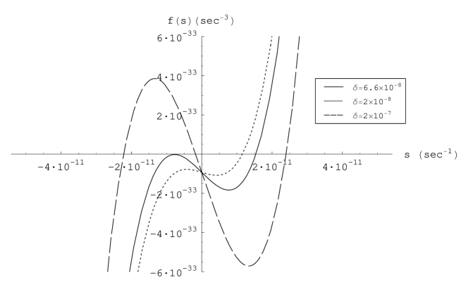
Figure 1: The function $f(s)$ for values of $q=q_{J}-\delta$ for a number density $n=10^{21}m^{-3}$ and temperature $T=10^{7}K$.

Analytically, the maximum for $s<0$ is given by

$$s_{-}=-\frac{\alpha}{3}-\frac{\sqrt{\alpha^{2}-3\beta}}{3}$$

and, since by varying $q$ the whole curve evolves with $f(0)$ virtually unchanged, the stability threshold is determined by $f(s_{-})=0$.

The second case we shall examine corresponds to lower values of density and temperature, i. e. $n=10^{12}m^{-3}$ and $T=10^{4}K$. The behavior in this case is quite different, as shown in Fig. 2. For these parameters, both $\alpha$ and the independent term are indeed negligible and thus, the critical value that gives the wave numbers is indicated by the disappearance of the two maxima. That is, the criterion can be found by imposing that the derivative of $f(s)$ has no real roots at all, i. e.

$$\beta>0$$

which, as clearly seen in Eq. (18) simply reduces to the ordinary Jeans criterion in absence of dissipation.

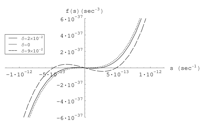
Figure 2: The function $f(s)$ for values of $q=q_{J}-\delta$ for a number density $n=10^{12}m^{-3}$ and temperature $T=10^{4}K$.

V Final Remarks

The problem of the gravitational instability including dissipative effects has been studied within the framework of linear irreversible thermodynamics, including cross effects, for a dilute binary plasma. The dissipative effects enter both the hydrodynamic equations and the dispersion relation for wave-like solutions of the linearized system.

The wave number for which perturbations start growing exponentially in time does not differ much form the standard Jeans wave number and thus, the response of the system to different fluctuations wavelengths is similar to the case with no dissipative effects present. However, the qualitative behavior of the dispersion relation in terms of $q$ is more complicated and has to be explored with care for each system. Cross effects are present in any multicomponent mixture and are enhanced by magnetic fields which are observed in many astrophysical systems key-4 ; key-7 . These effects, which are predicted by irreversible thermodynamics and kinetic theory, are in general not taken into account while studying gravitational stability and further analysis of them should be performed in the future.

- (1) S. R. de Groot and P. Mazur, “Non-Equilibrium Thermodynamics” (Dover Publications Inc., Mineola NY, 1984).
- (2) See for example: S. Weinberg, Ap. J. 168, 175 (1971); A. Sandoval-Villalbazo and L.S. García-Colín, Class. and Quan. Grav. 19, 2171 (2002); M. G. Corona-Galindo, H. Dehnen; Astrophys. Space Sci. 153, 87 (1989); A. Sandoval-Villalbazo and L.S. García-Colín, Physica A 347, 375 (2005).
- (3) S. Chapman and T. G. Cowling, “The Mathematical Theory of Non-Uniform Gases” (Cambridge Univ. Press, Cambridge, Third Edition 1970).
- (4) L. S. García-Colín, A. L. García-Perciante and A. Sandoval-Villalbazo; Phys. Plasmas 14, 012305 (2007).
- (5) L. Spitzer Jr., “The Physics of Fully Ionized Gases” (Wiley-Intescience Publ. Co, N. Y., 1962).
- (6) I. Braginski, “Transport Processes in a Plasma” Plasma Physics Reviews (Consultants Bureau Enterprise, N. Y., 1965)
- (7) W. Marshall; “The Kinetic Theory of an Ionized Gas”; U. K. A. E. A. Research Group, Atomic Energy Research Establishment, Harwell, U. K. (1960). R
- (8) Balescu, “Transport processes in plasmas Vol. I: classical transport theory” (Elsevier Science Ltd., 1988).for Astrophysics” (Princeton Univ. Press, Princeton, N. J., 2005)
- (9) P. Goldstein and L. S. García-Colín, J. Non-equilib. Thermodyn. 30, 173 (2005).