Microscopic Origin of Non-Gaussian Distributions of Financial Returns
Abstract
In this paper we study the possible microscopic origin of heavy-tailed probability density distributions for the price variation of financial instruments. We extend the standard log-normal process to include another random component in the so-called stochastic volatility models. We study these models under an assumption, akin to the Born-Oppenheimer approximation, in which the volatility has already relaxed to its equilibrium distribution and acts as a background to the evolution of the price process. In this approximation, we show that all models of stochastic volatility should exhibit a scaling relation in the time lag of zero-drift modified log-returns. We verify that the Dow-Jones Industrial Average index indeed follows this scaling. We then focus on two popular stochastic volatility models, the Heston and Hull-White models. In particular, we show that in the Hull-White model the resulting probability distribution of log-returns in this approximation corresponds to the Tsallis (t-Student) distribution. The Tsallis parameters are given in terms of the microscopic stochastic volatility model. Finally, we show that the log-returns for 30 years Dow Jones index data is well fitted by a Tsallis distribution, obtaining the relevant parameters.
1 Introduction
As any mature field, Finance has adopted a simple model developed over the years that attempts to describe the behaviour of random time fluctuations in the prices of commodities or stocks observed in the markets [1]. This model, which one could call the Standard Model of Finance (SMF), in spite of its many shortcomings has established a common language in a specific framework that immediately allows for generalizations. It predicts, for instance, prices for contracts on stocks, usually called derivative contracts [2]. The SMF assumes that the fluctuations of the stock prices follow a log-normal probability distribution function. It was first suggested by Osborne in 1959 [3] and independently by Samuelson [4], improving on an earlier model by guaranteeing non-negative stock prices.
In recent years, the large amount of financial data available has prompted many empirical investigations of the probability distributions of returns, defined as the logarithm of the ratio of stock prices separated by a given time lag. The simple log-normal assumption of the SFM would predict a Gaussian distribution for the returns with variance growing linearly with the time lag. What is actually found is that the probability distribution for high frequency data usually deviates from normality, presenting heavy tails. Fits have been made using the truncated Lévy distribution [5] and the so-called Tsallis (or t-Student) distribution [6].
An important question that we want to address is the nature of the microscopic stochastic process that may lead to these non-Gaussian distributions. For example, Borland proposed a feedback process where the diffusion coefficient is related to the macroscopic probability distribution, resulting in a non-linear Fokker-Planck equation whose solution is a time-dependent Tsallis distribution [7].
In this paper we study an extension of the SFM in which the diffusion of the stock price is itself represented by another independent stochastic process. In a very general way, one can divide these models into continuous- time stochastic volatility models and discrete-time Generalized Autoregressive Conditional Heteroskedasticity (GARCH) models [8]. Both classes can in principle describe some stylized facts such as volatility clustering [9]. The second class of models, used in standard econometric analysis, is based on time series data where previous values of the volatility and stock prices are used to calculate subsequent values.
In the following we will assume that volatility is not directly observed, and hence we will work in the context of the first class of models, where volatility can be interpreted as a hidden Markov process [10]. We show that in these stochastic volatility models there is a useful assumption that can be made and which results in probability distribution of returns with heavy tails and a simple scaling time dependence. In particular, we find that the Tsallis distribution follows from the Hull-White stochastic volatility model in this case. We test this assumption with daily data from the Dow Jones Industrial Average index and find a better agreement than the SFM.
2 Coupled stochastic processes for log-return and volatility
The price of a stock, , is a stochastic variable on the top of a deterministic exponential growth (with inflation rate ). It is therefore customary to regard the modified log-return,
| (1) |
as the indicator variable. It follows a Langevin equation of type
| (2) |
with being a Wiener process with zero mean and variance and is called the volatility. The function reflects the prescription when deriving the -process with additive noise from the -process with multiplicative noise. In the Ito-scheme it is . There exist, however, one particular Stratonovich scheme where it vanishes . Another possibility is to modify the equation (1) by adding a factor .
Equation (2) defines the SFM. An extension of the SFM considers the possibility that the variance itself is governed by stochastic effects, as suggested by phenomenological observations on financial markets [11]. The proposed models have a first order deterministic part causing an exponential approach to the mean volatility, and a noise term possibly influenced by the volatility itself:
| (3) |
The second Wiener process, , may or may not be correlated with the first one. We will consider two main models of stochastic volatility developed in the finance literature, namely the Heston and the Hull-White models. The Heston model uses [12] and in the Hull-White model [13].
Our purpose is to investigate approximations which enable a simplified treatment predicting the distribution of (or ) as a function of time.
3 Born-Oppenheimer approximation
Assuming that one of the coupled dynamical stochastic variables () reaches its stationary distribution and then acts for the dynamics of the other () as an instantaneous, time-independent background is analog to the Born-Oppenheimer (BO) approximation applied successfully in solid state and atomic physics. We will make this assumption in the remaining of the paper, explore its consequences and test it against data. The -process can be solved in itself; the corresponding Fokker-Planck equation is given as
| (4) |
The stationary detailed balance solution satisfies
| (5) |
The solution, the balance distribution of is given by
| (6) |
According to the BO-approximation we average over this stationary balance probability of the solution of the diffusion process of eq.(2) at a given ,
| (7) |
We obtain an approximation for the time evolution of the log-return probability:
| (8) |
Collecting all terms together we arrive at
| (9) |
4 Scaling in the BO approximation
In the case of a compensated Ito-term, i.e. , the dependence on the time lag in eq. (9) is via the combination and a in the normalization:
| (10) |
The scaling hypothesis (10) can be checked by detrending and normalizing the data. First one considers the log-return with a unit time-lag as
| (11) |
These values usually show a trend with the index for a fixed . We subtract the best fitted linear trend by the Gaussian least square method. From
| (12) |
it follows by derivation with respect to the fit parameters and :
| (13) |
From this we obtain
| (14) |
with
| (15) |
Next we compose the subtracted data as
| (16) |
These have by construction zero mean, () and zero index expectation value (). Finally the variance is normalized to one by considering
| (17) |
The we call (linearly) detrended and normalized log return data.
The distribution of these data is obtained by binning the values: the distance between the minimal and maximal is divided into intervals, so that is the beginning of the interval. Whenever a given is between and the counter is increased by one. The normalization is checked and is calculated. The normalized distribution is reconstructed as . We have tested the binning program with hoax data constructed from a normal Wiener process.
In order to check the scaling hypothesis we use the daily closing values of the Dow Jones Industrial Average (DJIA) index from January 1976 to December 2006, with data points and we adopt bins. In figure 1 we show the index time series and the detrended and normalized returns.
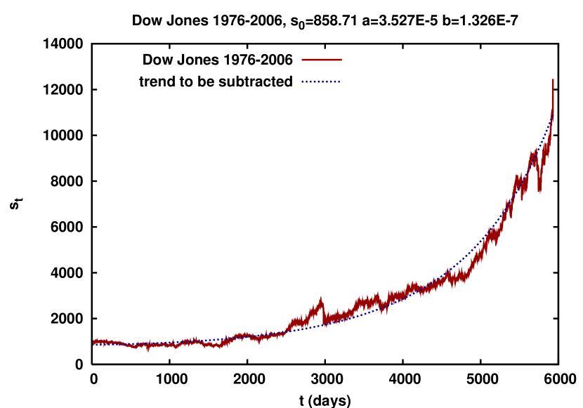
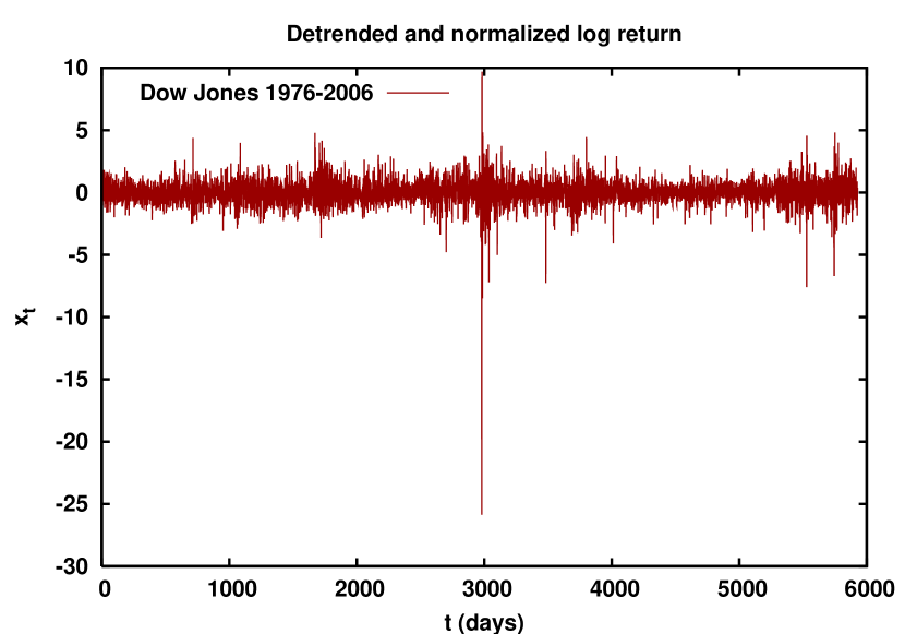
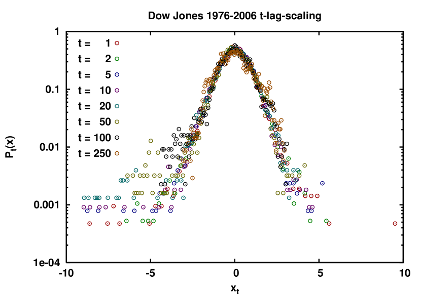
Figure 2 presents the detrended and normalized log-returns at different time-lags from 1 day to 250 days. The closeness of these data indicate that the scaling (detrending) is successful.
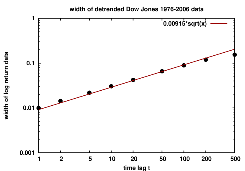
The universal scaling for case is (cf. eq.10)
| (18) |
for any time-lag . This is testable on the detrended data with different time-lags.
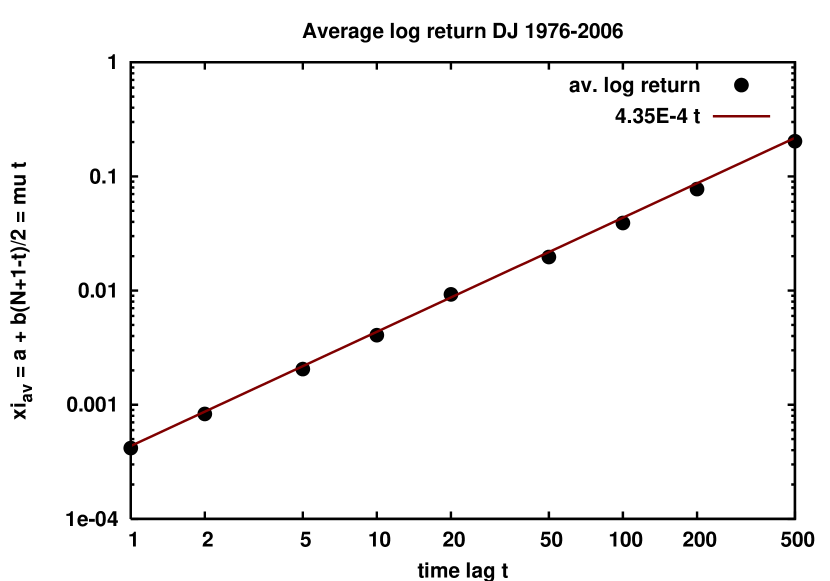
In Figure 3 the log returns for a given time lag show an average trend. The and parameters are obtained for several different time lags (from 1 to 500 days), as well as the width of detrended data before normalization. The average of on the top follows the straight line with meaning a yearly earnings (an average year had 5930/30=197 working days of the borse). The bottom picture shows the width of detrended data which is proportional to the square root of the time-lag on a double logarithmic scale. The fulfillment of this proportionality indicates that the scaling is realized by the data - since . This supports the BO approximation with .
5 Heston model in BO
The probability of returns in the Heston model has been extensively studied [14]. In the Heston model, and the stationary distribution is a Gamma distribution:
| (19) |
with . In the Ito-scheme and the above integral (9) can be determined analytically. The BO approximation corresponds to what ref. [14] calls the short time behaviour. Our basic assumption is that the volatility has already reached its stationary distribution. We obtain
| (20) |
with
| (21) |
and Bessel K-function. For large times . For large positive (extreme large wins on ) the Bessel function is dominated by an exponential, so
| (22) |
and for large negative (extreme losses) it is dominated by another exponential
| (23) |
Since at all times it means that in this model losses tend to show a fatter tail (slower decrease) in than wins. For short times, this difference reduces. Note that is a power-law behavior in , denoting by .
In the case of this model is also subject to the scaling as the normal diffusion. Now the factor is not present and in eq.(20). The distribution becomes symmetric for wins and losses (relative to the mean trend).
6 Hull-White model in BO
We now turn our attention to the probability distribution function resulting from the Hull-White stochastic volatility model in the BO approximation. To our knowledge this subject has not been discussed in the literature.
In the Hull-White model and the balanced volatility follows a Gamma-distribution in the reciprocal variable , the so-called inverse-Gamma distribution:
| (24) |
with . The BO-approximated distribution in the special scheme with becomes:
| (25) |
Regarding the quantity as an abstract “energy” the above formula represents a Boltzmann-Gibbs energy distribution under the influence of fluctuating “temperature”, which is identified with the variance. In particular a Gamma-distributed inverse temperature is known to lead to a cut power-law (Tsallis, or t-Student) distribution in the energy variable:
| (26) |
with
| (27) |
The quotient of functions constitutes Bernoulli’s Beta-function . A Gaussian distribution with variance given by is obtained in the limit, which can be thought of as the limit of a deterministic volatility ().
This result is symmetric in win and loss percentages, i.e. for all positive and negative values. As in the Heston model, asymmetries can be introduced by choosing a non-zero value of . On the other hand, it is easy to see that the large behavior is now a power-law in , not in . Nevertheless for large powers the cut power law distribution becomes quite close to the exponential for small and intermediate arguments, so the difference may influence the extreme large () values only.
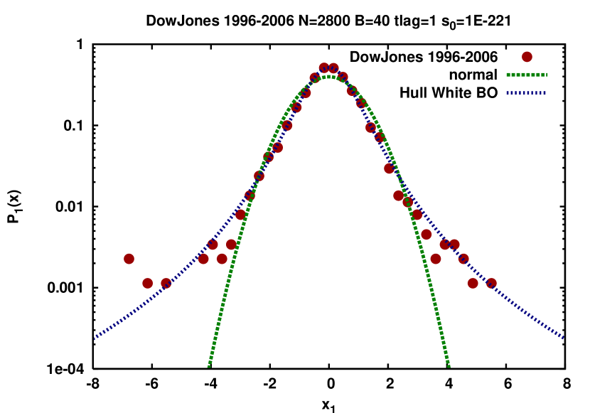
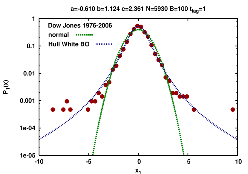
In Figure 4 we show a fit of the Hull-White model in the BO approximation for daily returns of the DJIA index. We find and . One can see that the resulting Tsallis distribution provides a much better fit compared to the usual Gaussian model for the log-returns. It is important to notice that the parameters for the Tsallis distribution are directly related to the Hull-White stochastic volatility model, providing a microscopic origin for this non-Gaussian distribution.
7 Discussion and Conclusions
It has been known for quite sometime that the distribution of returns are not Gaussian, as assumed by the SFM. What has been the subject of some debate in the literature is the nature of the processes that cause this deviation from normality.
Our results have shown that the observed non-Gaussian, fat-tailed distribution of returns can be obtained microscopically by two coupled independent stochastic processes, one for the returns and the other for the volatility of the returns. In our analysis we assumed that the stochastic volatility process quickly reaches a stationary distribution and acts as a background for the return process. We then obtain the distribution of the returns by integrating over the instantaneous volatility that is distributed according to the stationary distribution. This is analogous to the Born-Oppenheimer approximation in Physics and we showed that it leads in this case to satisfactory results. In particular, we demonstrated that all models of stochastic volatility should exhibit a scaling relation in the time lag of zero-drift modified log-returns and we verified that the Dow-Jones Industrial Average index indeed follows this scaling from time lags of of 1 day up to 500 days, beyond which data becomes sparse.
We provided a microscopic explanation for a Tsallis distribution of log-returns. The parameters of a microscopic Hull-White stochastic volatility model uniquely determine the parameters of the macroscopic Tsallis distribution. We estimated these parameters from a fit to 30 years Dow Jones index daily data, concluding that they do result in a much better agreement than the SMF Gaussian distribution. Since the scaling is observed in the data, this daily fit determines the distribution for all other time lags. The transition to Gaussian distributions for large time lags occurs because the fat tails are pushed away as the distribution broadens with time and the central region of the distribution is well described by a Gaussian distribution. This can be seen by expanding eq.(26) for large time lags, a well known fact in the literature [15].
In a more general approach one should attemp to reconstruct directly and from data, which is tantamount to reconstruct the best stochastic volatility model compatible with data. This attempt is analogous to deciphering the Planck distribution and hence the temperature for distant stars from their radiation spectra. In this respect the BO approximation used in the Hull-White model should be viewed as yet another particular model and as such it should be tested. This was pursued in this paper.
Acknowledgments
We would like to thank János Kertész and especially Victor Yakovenko for a very careful reading of the paper and many discussions about the assumptions made. R. Rosenfeld thanks CNPq for partial financial support. T. S. Biró acknowledges the warm hospitality of the IFT at UNESP, São Paulo, Brazil, and the partial support by the Hungarian National Research Fund OTKA (T49466).
References
- [1] For an introduction, see e.g., J. C. Hull, Options, Futures and Other Derivatives, 6th edition, Prentice Hall (2005).
- [2] F. Black and M. Scholes, J. Pol. Econ. 81, 673 (1973).
- [3] M. F. M. Osborne, Operations Research 7, 145 (1959); see also M. F. M. Osborne, The Stock Market and Finance from a Physicist’s Viewpoint, Crossgar Press (1996).
- [4] For a very interesting account of the development of the SMF, see M. S. Taqqu, in Mathematical Finance, Bachelier Congress 2000, H. Geman et al. (Editors), Springer (2002).
- [5] R. N. Mantegna and H. E. Stanley, Nature 376, 46 (1995); see also R. N. Mantegna and H. E. Stanley, Introduction to Econophysics: Correlations and Complexity in FInance, Cambridge University Press (2000).
- [6] C. Tsallis, C. Anteneodo, L. Borland and R. Osorio, Physica A 324, 89 (2003).
- [7] L. Borland, Phys. Rev. Lett. 89, 098701 (2002); L. Borland, Quant. Finance 2, 415 (2002).
- [8] S. L. Heston and S. Nandi, Rev. Financial Stud. 13, 585 (2000).
- [9] Z. Eisler and J. Kertesz, Eur. Phys. J. B 51, 145 (2006); Phys. Rev. E 73, 046109 (2006).
- [10] Z. Eisler, J. Perelló and J. Masoliver, arXiv:physics/0612084.
- [11] For a phenomenological evidence and calibration of stochastic volatility models see, e.g., S. Miccichè, G. Bonanno, F. Lillo and R. N. Mantegna, Physica A 314, 756 (2002); R. Remer and R. Mahnke, Physica A 344, 236 (2004).
- [12] S. L. Heston, Rev. Financial Stud. 6, 327 (1993).
- [13] J. Hull and A. White, J. Finance XLII, 281 (1987).
- [14] A. A. Dragulescu and V. M. Yakovenko, Quantitative Finance 2, 443 (2002).
- [15] See, e.g., A. C. Silva and V. M. Yakovenko, Physica A 382, 278 (2007).