DESY 07-068

On Newton’s law in supersymmetric braneworld models

Gonzalo A. Palma

Deutsches Elektronen-Synchrotron DESY, Theory Group, Notkestrasse 85, D-22603 Hamburg, Germany

Abstract

We study the propagation of gravitons within 5-D supersymmetric braneworld models with a bulk scalar field. The setup considered here consists of a 5-D bulk spacetime bounded by two 4-D branes localized at the fixed points of an $S^{1}/\mathbb{Z}_{2}$ orbifold. There is a scalar field $\phi$ in the bulk which, provided a superpotential $W(\phi)$, determines the warped geometry of the 5-D spacetime. This type of scenario is common in string theory, where the bulk scalar field $\phi$ is related to the volume of small compact extra dimensions. We show that, after the moduli are stabilized by supersymmetry breaking terms localized on the branes, the only relevant degrees of freedom in the bulk consist of a 5-D massive spectrum of gravitons. Then we analyze the gravitational interaction between massive bodies localized at the positive tension brane mediated by these bulk gravitons. It is shown that the Newtonian potential describing this interaction picks up a non-trivial contribution at short distances that depends on the shape of the superpotential $W(\phi)$. We compute this contribution for dilatonic braneworld scenarios $W(\phi)\propto e^{\alpha\phi}$ (where $\alpha$ is a constant) and discuss the particular case of 5-D Heterotic M-theory: It is argued that a specific footprint at micron scales could be observable in the near future.

1 Introduction

Recent tests of gravity at short distances [1, 2, 3, 4] have confirmed that Newton’s inverse-square law holds down to a length scale $56\mu$m. This has substantially improved previous constraints on exotic interactions mediated by the exchange of massive scalars or vectors between neutral atoms [5], where a Yukawa type contribution to the Newtonian potential is generally expected. It has also lowered the scale at which large extra dimensions [6, 7, 8] and braneworld models [9, 10, 11] may show up by affecting the propagation of gravitons in the presence of a large –or infinite– extra dimensional volume.

Indeed, in theories where matter fields confine to a 4-D brane and gravity is the only massless field able to propagate along the extra dimensional volume [12, 13, 14], one generally expects short distance corrections to the usual 4-D Newtonian potential. The shape and distance at which these corrections become relevant generally depend on the geometry and size of the extra dimensional volume, thus allowing for distinctive signals dependent of the particular content of the theory. In the single-brane Randall-Sundrum scenario [11], for instance, where a 4-D brane of constant tension $\propto k$ is immersed in an infinitely large five-dimensional AdS volume, a zero mode graviton $g_{\mu\nu}$ localizes about the brane. This zero mode is exponentially suppressed away from the brane with a warp factor $\propto e^{-kz}$, where $z$ is the distance from the brane along the fifth extra-dimensional direction. The Newtonian potential describing the gravitational interaction between two bodies of masses $m_{1}$ and $m_{2}$ localized at the brane, and separated by a distance $r$, is then found to be [11, 15, 16, 17, 18]

$$V(r)=-G_{\mathrm{N}}\frac{m_{1}m_{2}}{r}\Big{(}1+\frac{2}{3k^{2}r^{2}}\Big{)},$$ (1)

where $G_{\mathrm{N}}$ is Newton’s constant. The correction $2/3k^{2}r^{2}$ springs out directly from the way in which bulk gravitons propagate in an AdS five-dimensional spacetime. A correction like this provides an important signature for the low energy phenomenology of braneworld models with warped extra-dimensions; if the tension $k$ is small enough as compared to the Planck mass $M_{\mathrm{Pl}}=(8\pi G_{\mathrm{N}})^{-1/2}$, then it would be possible to distinguish this type of scenario from other extra-dimensional models in up-coming short distance tests of gravity (present tests give the robust constraint $1/k<11\mu$m).

It is therefore sensible to ask how other braneworld scenarios may differ from the Randall-Sundrum case at short distances, especially within the context of more realistic models. The purpose of this paper is to shed light towards this direction. Here we study the propagation of gravitons within 5-D braneworld models where the geometry of the extra-dimensional space differs from the usual AdS profile. We will show that the gravitational interaction at short distances is sensitive to the geometry of the extra-dimensional bulk in such a way that the Newtonian potential picks up a non-trivial correction at scales comparable to the tension of the brane. As we shall see, this correction may differ dramatically from the one depicted in Eq. (1). We refer to [19, 20, 21, 22, 23, 24, 25, 26] for other works on short distance modifications to general relativity within the braneworld paradigm.

1.1 General idea

We will look into a fairly general class of supersymmetric braneworld scenarios with a bulk scalar field $\phi$. The model considered here consists of a 5-D bulk spacetime bounded by two 4-D branes localized at the fixed points of an $S^{1}/\mathbb{Z}_{2}$ orbifold. The tensions of the branes are proportional to the superpotential $W(\phi)$ of the theory, allowing for BPS configurations in which half of the bulk supersymmetry is broken on the branes [27, 28]. These types of models are well motivated from string theory, particularly within the heterotic M-theory approach [29, 30] where, in the 5-D effective low energy theory, the scalar field $\phi$ is related to the size of the volume of small extra-dimensions compactified on a Calabi-Yau 3-fold [31, 32]. To gain insight into the gravitational phenomenology of this model, we shall only consider the bosonic sector of the theory.

One crucial property for us coming from this class of models is that the warping of the extra-dimensional volume depends on the form of the superpotential $W(\phi)$. To be more precise, given a metric $g_{\mu\nu}=\omega^{2}(z)\eta_{\mu\nu}$, where $\eta_{\mu\nu}$ is the usual Minkowski metric and $z$ is the coordinate parameterizing the proper distance along the extra-dimension, then bulk fields are related to $W(\phi)$ by means of the following first order differential equations

$$\frac{\omega^{\prime}}{\omega}=-\frac{1}{4}W\qquad\mathrm{and}\qquad\phi^{\prime}=\frac{\partial W}{\partial\phi},$$ (2)

where ${}^{\prime}\equiv\partial_{z}$. In the particular case of Randall-Sundrum branes, the superpotential is simply a constant $W=4k$, implying an AdS5 spacetime with $\omega=e^{-kz}$. For more general superpotentials, however, the warping of the extra-dimension may have a richer structure and even contain singularities [33]. For example, in the case of dilatonic braneworlds, where $W(\phi)=\Lambda\,e^{\alpha\phi}$, one encounters a singularity $\omega=0$ at a distance $z=1/\alpha^{2}W(\phi_{1})$ from the positive tension brane, where $\phi_{1}$ is the value that the scalar field acquires on the brane. In this way, while in the Randall-Sundrum model there is a positive-tension brane in an infinite volume (with $\omega=0$ at infinity), in more general cases one may have a single positive-tension brane immersed in a finite bulk-volume at a certain distance from the $\omega=0$ singularity.

The basic idea of this paper is to compute the effect of such geometries on the gravitational interaction between massive bodies localized on the same brane. For simplicity, we shall consider single-brane configurations in which the visible brane corresponds to the positive tension brane, whereas the negative tension brane localizes at the bulk singularity.

1.2 The moduli problem

Models with extra-dimensions generically predict the existence of massless degrees of freedom, the moduli, at the 4-D effective theory level [15, 34]. These moduli appear coupled to the matter sector with the same strength as gravity, leading to significant long range modifications to general relativity, well constrained by both Solar system [35, 36, 37] and binary pulsar tests [38, 39, 40, 41]. In the Randall-Sundrum model, the radion moduli vanishes as the negative tension brane disappears at infinity –the single brane limit– leaving gravity as the only relevant long range interaction of the model. However, in more general braneworld scenarios –as the one we consider here– one typically expects other massless degrees of freedom, even in the single brane limit. For instance, current Solar system tests imply a constraint on the following dimensionless parameter $\alpha\equiv W^{-1}\partial_{\phi}W$

$$\alpha^{2}<1.5\times 10^{-6},$$ (3)

where $\alpha$ is evaluated on the brane in which tests are performed [42]. The Randall-Sundrum model corresponds to the trivial case $\alpha^{2}=0$, thus passing the test with flying colors, nevertheless, in more realistic models one has $\alpha^{2}\simeq\mathcal{O}(1)$. As we shall learn later in more detail, in order to have significant effects at short distances –say, at micron scales– different from the Randall-Sundrum case, it is necessary to be in the range $\alpha^{2}\simeq\mathcal{O}(1)$. This strongly contrasts with the bound of Eq. (3).

One way out of this problem consists in taking into account a stabilization mechanism for the moduli [43, 44], in this case, for the bulk scalar field $\phi$. If $\phi$ becomes massive on the branes, then the only relevant long range interaction in the bulk would consists of the gravitational field. To this extent, we consider supersymmetry breaking potentials localized at the orbifold fixed points. We will show that, provided certain simple conditions on these potentials, it is possible to stabilize the bulk scalar field $\phi$ without spoiling the vacuum geometry of the extra-dimensional space dictated by Eq. (2), and therefore retaining all the interesting features coming from the bulk-curvature.

1.3 Plan of the paper

This work is organized in the following way: We start in Section 2 by introducing braneworld models with a bulk scalar field. There, we deduce the equations of motion of the system and present the zero mode background solution –a BPS vacuum state– and its effective theory, a bi-scalar-tensor theory of gravity. The scalar degrees of freedom of this theory consist of the boundary values of $\phi$ at both branes. Then in Section 3 we study the linear perturbations of the fields around the zeroth-order solution presented in Section 2. There, we also consider the problem of stabilizing the moduli. We show that, once the zeroth-order moduli are stabilized, the only relevant degrees of freedom at low energies in the bulk consist of a massive tower of 5-D gravitons. In Section 4 we analyze the effects of these massive states on the gravitational interaction between massive bodies localized at the same brane. There, we compute the short distance modifications to Newton’s inverse-square law parameterized by a function $f(r)$ appearing in the form

$$V(r)=-G_{\mathrm{N}}\frac{m_{1}m_{2}}{r}\left[1+f(r)\right].$$ (4)

As we shall see, the shape of the function $f(r)$ depends heavily on the shape of the superpotential $W(\phi)$. To put things into context, we further compute the corrections arising in the particular case of dilatonic braneworlds $W(\phi)\propto e^{\alpha\phi}$, where $\alpha$ is a constant. There, we also discuss the particular case of 5-D Heterotic M-Theory and the prospects of observing these corrections in the near future. Finally, in Section 5 we provide some concluding remarks.

2 Braneworld models with a bulk scalar field

Let us consider a 5-D spacetime $M$ with topology $M=\mathbb{R}^{4}\times S^{1}/\mathbb{Z}_{2}$, where $\mathbb{R}^{4}$ is a fixed 4-D Lorentzian manifold without boundaries and $S^{1}/\mathbb{Z}_{2}$ is the orbifold constructed from the one-dimensional circle with points identified through a $\mathbb{Z}_{2}$-symmetry. $M$ is bounded by two 3-branes located at the fixed points of $S^{1}/\mathbb{Z}_{2}$. We denote the brane hyper-surfaces by $\Sigma_{1}$ and $\Sigma_{2}$ respectively, and call the space $M$ bounded by the branes, the bulk space. In this model there is a bulk scalar field $\phi$ with a bulk potential $U(\phi)$ and boundary values $\phi^{1}$ and $\phi^{2}$ at the branes. Additionally, the branes have tensions $\lambda_{1}$ and $\lambda_{2}$ which are given functions of $\phi^{1}$ and $\phi^{2}$, respectively (see Fig. 1).

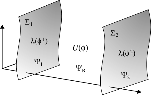
Figure 1: Schematic representation of the 5-D brane configuration. In the bulk there is a scalar field $\phi$ with a bulk potential $U(\phi)$. Additionally, the bulk space is bounded by branes $\Sigma_{1}$ and $\Sigma_{2}$ located at the orbifold fixed points. The branes are characterized by tensions $\lambda_{1}$ and $\lambda_{2}$, and contain matter fields $\Psi_{1}$ and $\Psi_{2}$ respectively.

The total action of the system is given by

$$S_{\mathrm{tot}}=S_{\mathrm{bulk}}+S_{\mathrm{brane}},$$ (5)

where $S_{\mathrm{bulk}}$ is the term describing the gravitational physics at the bulk (including the bulk scalar field)

$$S_{\mathrm{bulk}}=\frac{M_{5}^{3}}{2}\int_{M}\!R^{(5)}-\frac{3M_{5}^{3}}{8}\int_{M}\!\left[(\partial\phi)^{2}+U(\phi)\right]+S_{\mathrm{GH}}.$$ (6)

Here the integral symbol $\int$ is the short notation for $\int d^{5}X\sqrt{-g_{5}}$, where $X^{A}$, with $A=1,\cdots,5$, is the coordinate system covering $M$ and $g_{5}$ is the determinant of the 5-D metric $g_{AB}$ of signature $(-++++)$. $M_{5}$ is the 5-D fundamental mass scale and $R^{(5)}$ is the 5-D Ricci scalar. Observe that in the present notation the bulk scalar field $\phi$ is dimensionless. The third term of Eq. (6) corresponds to the Gibbons-Hawking boundary term $S_{\mathrm{GH}}\propto\int_{\Sigma_{1}}K-\int_{\Sigma_{2}}K$, added to make the bulk gravitational physics regular near the fixed points. The action $S_{\mathrm{brane}}$ appearing in Eq. (5) stands for the fields at the fixed points. It is given by

$$S_{\mathrm{brane}}=S_{\mathrm{matter}}-\frac{3M_{5}^{3}}{2}\,\int_{\Sigma_{1}}\!\lambda_{1}(\phi^{1})-\frac{3M_{5}^{3}}{2}\,\int_{\Sigma_{2}}\!\lambda_{2}(\phi^{2}),$$ (7)

where $\lambda_{1}(\phi^{1})$ and $\lambda_{2}(\phi^{2})$ are the brane tensions and $S_{\mathrm{matter}}$ the action describing the matter content of the branes, which we write

$$S_{\mathrm{matter}}=S_{1}[\Psi_{1},g_{\mu\nu}^{(1)}]+S_{2}[\Psi_{2},g_{\mu\nu}^{(2)}],$$ (8)

where $\Psi_{1}$ and $\Psi_{2}$ denote the matter fields at each brane, and $g_{\mu\nu}^{(1)}$ and $g_{\mu\nu}^{(2)}$ are the induced metrics at $\Sigma_{1}$ and $\Sigma_{2}$ respectively. In what follows we summarize some important properties of this system.

2.1 5-D supergravity

As already mentioned, we focus our interest on a class of models embedded in supergravity, where the bulk potential $U(\phi)$ and the brane tensions $\lambda_{1}(\phi^{1})$ and $\lambda_{2}(\phi^{2})$ satisfy a special relation so as to preserve half of the local supersymmetry near the branes [27]. The relation turns out to be

$$U=(\partial_{\phi}W)^{2}-W^{2},\qquad\lambda_{1}=W(\phi^{1}),\qquad\mathrm{and}\qquad\lambda_{2}=-W(\phi^{2}),$$ (9)

where $W=W(\phi)$ is the superpotential of the system. Observe that the tensions $\lambda_{1}$ and $\lambda_{2}$ depend on $W$ with opposite signs.

Several aspects of this class of models have been thoroughly investigated over the last few years, among them: Braneworld inflation [45, 46, 47], their low energy dynamics [48, 49, 50, 51, 52, 53, 54], brane collisions [55, 56], and various phenomenological aspects [57, 58, 59]. This class of model is attractive for several reasons: On the one hand, they offer a natural extension to the much studied Randall-Sundrum model, where a fine tuning condition between the bulk cosmological constant and the tensions allows a null effective cosmological constant on the brane. This is also the case here [60, 61, 62, 63] where condition (9) implies a zero effective dark energy term on the brane. In fact, the case $W=$ constant corresponds to the particular case of Randall-Sundrum branes. On the other hand, this is the generic class of models one would expect from superstring theories, where the size of the volume of compactified extra-dimensions is modeled as a scalar field. For example, in low energy Heterotic M-theory it is found, after compactifying 6 of the 10 spatial dimensions on a Calabi-Yau 3-fold [32], a superpotential of the form $W(\phi)\propto e^{\alpha\phi}$, with $\alpha^{2}=3/2$.

Since in the real world supersymmetry is expected to be broken, it is convenient to consider small deviations from the configuration of Eq. (9). We do this by introducing supersymmetry breaking potentials $v_{1}(\phi^{1})$ and $v_{2}(\phi^{2})$ at the branes in the following way

$$U=(\partial_{\phi}W)^{2}-W^{2},\qquad\lambda_{1}=W+v_{1},\qquad\mathrm{and}\qquad\lambda_{2}=-W-v_{2},$$ (10)

with $|v_{1}|\ll|W(\phi^{1})|$ and $|v_{2}|\ll|W(\phi^{2})|$. Potentials $v_{1}(\phi^{1})$ and $v_{2}(\phi^{2})$ parameterize deviations from the BPS condition (9). The precise mechanism by which they are generated is out of the scope of the present work. We refer to [64, 65] for discussions on this issue.

2.2 4-D covariant formulation

Given the topology $M=\mathbb{R}^{4}\times S^{1}/\mathbb{Z}_{2}$, it is convenient to decompose the coordinate system $X^{A}$ into $(x^{\mu},z)$, where $x^{\mu}$ with $\mu=1,\cdots,4$ covers the $\mathbb{R}^{4}$ foliations and surfaces $\Sigma_{1}$ and $\Sigma_{2}$, and where $z$ covers the $S^{1}/\mathbb{Z}_{2}$ orbifold and parameterizes the 4-D foliations. With this decomposition, it is customary to write the metric line element $ds^{2}=g_{AB}dX^{A}dX^{B}$ as

$$ds^{2}=N^{2}dz^{2}+g_{\mu\nu}(dx^{\mu}+N^{\mu}dz)(dx^{\nu}+N^{\nu}dz).$$ (11)

Here, $N$ and $N^{\mu}$ are the lapse and shift functions for the extra dimensional coordinate $z$, and $g_{\mu\nu}$ is the induced metric on the 4-D foliations with a $(-+++)$ signature. At the boundaries we have $g_{\mu\nu}^{(1)}=g_{\mu\nu}(z_{1})$ and $g_{\mu\nu}^{(2)}=g_{\mu\nu}(z_{2})$. It is possible to show that the unit-normal vector $n^{A}$ to the foliations has components

$$n^{A}=(-N^{\mu}/N,1/N),\qquad n_{A}=(0,N).$$ (12)

Additionally, it is useful to define the extrinsic curvature $K_{\mu\nu}$ of the 4-D foliations as

$$K_{\mu\nu}=\frac{1}{2N}\left[g_{\mu\nu}^{\prime}-\nabla_{\mu}N_{\nu}-\nabla_{\nu}N_{\mu}\right],$$ (13)

where ${}^{\prime}=\partial_{z}$ and covariant derivatives $\nabla_{\mu}$ are constructed from the induced metric $g_{\mu\nu}$ in the standard way. Another way of writing the extrinsic curvature is $2NK_{\mu\nu}=\pounds_{Nn}g_{\mu\nu}$, where $\pounds_{Nn}$ is the Lie derivative along the vector field $Nn^{A}$.

The present notation allows us to reexpress $S_{\mathrm{bulk}}$ of Eq. (6) in the following way

$$S_{\mathrm{bulk}} = \frac{M_{5}^{3}}{2}\int_{S^{1}\!/\mathbb{Z}_{2}}\!\!\!\!\!\!\!dz\!\int\!\!d^{\,4}x\sqrt{-g}\,N\bigg{(}R-[K_{\mu\nu}K^{\mu\nu}-K^{2}]-\frac{3}{4}\big{[}(\phi^{\prime}/N)^{2}$$ (14)

$$+(g^{\mu\nu}+N^{\mu}N^{\nu}/N^{2})\partial_{\mu}\phi\partial_{\nu}\phi-2N^{-2}N^{\mu}\,\partial_{\mu}\phi\,\partial_{z}\phi+U\big{]}\bigg{)},$$

where $R$ is the four-dimensional Ricci scalar constructed from $g_{\mu\nu}$ and $K=g^{\mu\nu}K_{\mu\nu}$ is the trace of the extrinsic curvature. Observe that the Gibbons-Hawking boundary term $S_{\mathrm{GH}}$, which appeared originally in $S_{\mathrm{bulk}}$, has been absorbed by the use of metric (11). Let us clarify here that the integration in Eq. (14) along the fifth-dimension is performed on the entire circle $S^{1}$, instead of just half of it. We should keep in mind, however, that degrees of freedom living in different halves of the circle are identified through the $\mathbb{Z}_{2}$-symmetry.

2.3 Dynamics and boundary conditions

In this section we deduce the equations of motion governing the dynamics of the fields living in the bulk and the branes. These equations are obtained by varying the total action of the system $S_{\mathrm{tot}}$ with respect to the bulk gravitational fields $N$, $N^{\mu}$, $g_{\mu\nu}$ and $\phi$, taking special care on the variation of the boundary terms. The brane tensions $\lambda_{1}$ and $\lambda_{2}$ and matter fields $\Psi_{1}$ and $\Psi_{2}$ play a decisive role in determining boundary conditions on the bulk gravitational fields at $\Sigma_{1}$ and $\Sigma_{2}$, respectively. The variation of $S_{\mathrm{tot}}$ with respect to $N$, $N^{\mu}$ and $g_{\mu\nu}$ respectively, gives

$$R+\left[K_{\mu\nu}K^{\mu\nu}-K^{2}\right]=-\frac{3}{4}\bigg{[}\frac{1}{N^{2}}(\phi^{\prime})^{2}-g^{\mu\nu}\partial_{\mu}\phi\partial_{\nu}\phi-U\bigg{]},$$ (15)

$$\nabla_{\mu}\left[K^{\mu}_{\nu}-K\delta^{\mu}_{\nu}\right]=\frac{3}{4}\frac{1}{N}\phi^{\prime}\partial_{\mu}\phi,$$ (16)

$$G_{\mu\nu}=\frac{1}{N}(\nabla_{\mu}\nabla_{\nu}N-g_{\mu\nu}\Box N)-\frac{1}{2}g_{\mu\nu}\left[K_{\rho\sigma}K^{\rho\sigma}+K^{2}\right]+\frac{1}{N}(K_{\mu\nu}-g_{\mu\nu}K)^{\prime}$$

$$+3KK_{\mu\nu}-2K_{\mu\alpha}K^{\alpha}_{\,\,\nu}-\frac{3}{8}g_{\mu\nu}\left[(\phi^{\prime}/N)^{2}+g^{\mu\nu}\partial_{\mu}\phi\partial_{\nu}\phi+U\right]+\frac{3}{4}\partial_{\mu}\phi\partial_{\nu}\phi.$$ (17)

To write these equations we have adopted Gaussian normal coordinates, which correspond to the gauge choice $N^{\mu}=0$ (with this gauge one has $\pounds_{Nn}=\partial_{z}$). Here $G_{\mu\nu}=R_{\mu\nu}-\frac{1}{2}g_{\mu\nu}R$ is the Einstein tensor constructed out from the induced metric $g_{\mu\nu}$. The bulk scalar field equation of motion can be deduced either from the previous set of equations (by exploiting energy momentum conservation), or just by varying the action $S_{\mathrm{tot}}$ with respect to $\phi$. One obtains

$$\left[\nabla^{\mu}\left(N\partial_{\mu}\phi\right)+\left(\phi^{\prime}/N\right)^{\prime}+K\phi^{\prime}\right]=\frac{N}{2}\frac{\partial U}{\partial\phi}.$$ (18)

Near the branes the variation of the action leads to a set of boundary conditions known as the Israel matching conditions [66]. In the present model, they are given by

$$K_{\mu\nu}-g_{\mu\nu}K = \frac{3}{4}\lambda_{1}\,g_{\mu\nu}-\frac{1}{2}M_{5}^{-3}T_{\mu\nu}^{1},$$ (19)

$$\phi^{\prime} = N\,\partial_{\phi}\lambda_{1},$$ (20)

at the first brane $\Sigma_{1}$, and

$$K_{\mu\nu}-g_{\mu\nu}K = -\frac{3}{4}\lambda_{2}\,g_{\mu\nu}+\frac{1}{2}M_{5}^{-3}T_{\mu\nu}^{2},$$ (21)

$$\phi^{\prime} = -N\,\partial_{\phi}\lambda_{2},$$ (22)

at the second brane $\Sigma_{2}$. In the previous expressions we have defined the 4-D energy-momentum tensors $T^{1}_{\mu\nu}$ and $T^{2}_{\mu\nu}$ describing $\Psi_{1}$ and $\Psi_{2}$ in the conventional way

$$T^{1}_{\mu\nu}=-\frac{2}{\sqrt{-g}}\frac{\delta S_{1}}{\delta g^{\mu\nu}}\bigg{|}_{z_{1}}\qquad\mathrm{and}\qquad T^{2}_{\mu\nu}=-\frac{2}{\sqrt{-g}}\frac{\delta S_{2}}{\delta g^{\mu\nu}}\bigg{|}_{z_{2}},$$ (23)

where $S_{1}$ and $S_{2}$ are the terms appearing in the action $S_{\mathrm{brane}}$ of Eq. (8).

2.4 BPS solutions

Let us, for a moment, assume that the supersymmetry breaking potentials $v_{1}(\phi^{1})$ and $v_{2}(\phi^{2})$ defined in Section 2.1 and brane matter fields $\Psi_{1}$ and $\Psi_{2}$ are absent. Then, given a superpotential $W(\phi)$, the bulk scalar field potential and brane tensions become

$$U=(\partial_{\phi}W)^{2}-W^{2},\qquad\lambda_{1}=W(\phi^{1}),\qquad\mathrm{and}\qquad\lambda_{2}=-W(\phi^{2}).$$ (24)

Under these conditions the system presents an important property which shall be exploited heavily during the rest of the paper: The system has a BPS vacuum state consisting of a static bulk background in which branes can be allocated anywhere, without obstruction. Indeed, suppose that the bulk fields depend only on $z$, and write $g_{\mu\nu}=\omega^{2}(z)\eta_{\mu\nu}$, where $\eta_{\mu\nu}$ is the Minkowski metric, then one finds that the entire system of equations (15)-(18) are solved by functions $\omega(z)$ and $\phi(z)$ satisfying

$$\frac{\omega^{\prime}}{\omega}=-\frac{N}{4}W\qquad\mathrm{and}\qquad\phi^{\prime}=N\partial_{\phi}W.$$ (25)

Remarkably, boundary conditions (19)-(22) are also given by these two equations. Thus, the presence of the branes forces the system to aquire a domain-wall-like vacuum background, instead of a flat 5-D Minkowski background. This property allows us to handle the complicated system of equations (15)-(18) by linearizing fields about this state. This will be considered in detail in Section 3.

Notice that the warp factor $\omega(z)$ may be solved and expressed as a function of $\phi(z)$ instead of $z$

$$\omega(\phi)=\exp\left[-\frac{1}{4}\int^{\phi}\!\!\!\alpha^{\!-1}(\phi)\,d\phi\right],\qquad\mathrm{where}\qquad\alpha(\phi)\equiv\frac{\partial_{\phi}W}{W}.$$ (26)

2.4.1 Dilatonic braneworlds

In the case of dilatonic braneworlds one has $W=\Lambda\,e^{\alpha\phi}$, where $\Lambda$ is a mass scale expected to be of order $M_{5}$, and $\alpha$ is a dimensionless constant. In this case the relations of Eq. (25) permit us to solve the background values $\phi$ and $\omega$ in terms of $z$. Using the gauge $N=1$ for definiteness and assuming $\Lambda>0$, one obtains

$$\phi(z) = \phi_{1}-\frac{1}{\alpha}\ln\left[1-\alpha^{2}W_{0}z\right],$$ (27)

$$\omega(z) = \left[1-\alpha^{2}W_{0}z\right]^{1/4\alpha^{2}},$$ (28)

where $\phi_{1}\equiv\phi(0)$ and $W_{0}=\Lambda\,e^{\alpha\phi_{1}}$. Notice the presence of a singularity $\omega=0$ at $z=1/\alpha^{2}W_{0}$. Without loss of generality, one may take the position of the first brane $\Sigma_{1}$ at $z=0$ (since $\Lambda>0$, this is a positive tension brane). Then, the second brane $\Sigma_{2}$ can be anywhere between $z=0$ and $z=1/\alpha^{2}W_{0}$. Later on, we shall study the case in which $\Sigma_{2}$ is stabilized at the singularity.

2.5 Effective theory

To finish, we present the effective theory describing the dynamics for the zeroth-order fields from the 4-D point of view. The effective theory is a bi-scalar tensor theory of gravity of the form [52, 51]

$$S = \frac{1}{4\pi G_{*}}\int d^{4}x\sqrt{-g}\bigg{[}\frac{1}{4}R-\frac{1}{2}g^{\mu\nu}\gamma^{ab}\partial_{\mu}\omega_{a}\partial_{\nu}\omega_{b}-V\bigg{]}$$ (29)

$$+S_{1}[\Psi_{1},A_{1}^{2}g_{\mu\nu}]+S_{2}[\Psi_{2},A_{2}^{2}g_{\mu\nu}],\qquad$$

where $\omega_{a}$, with $a=1,2$, are the values of the warp factor $\omega(z)$ at the brane positions $z_{a}$ and $G_{*}^{-1}\equiv 16\pi M_{5}^{2}$. Observe that $\omega_{a}$ can be expressed in terms of $\phi^{a}$ (the boundary values of $\phi$) by using Eq. (26) evaluated at $\phi=\phi^{a}$. The elements of the sigma model metric $\gamma^{ab}$ are given by

$$\gamma^{11}=-\frac{6M_{5}}{B^{2}W_{1}}\bigg{[}1-\frac{2M_{5}A_{1}^{2}}{W_{1}}\bigg{]},\qquad\gamma^{22}=+\frac{6M_{5}}{B^{2}W_{2}}\bigg{[}1+\frac{2M_{5}A_{2}^{2}}{W_{2}}\bigg{]},$$

$$\gamma^{12}=\gamma^{21}=-\frac{12M_{5}^{2}\omega_{1}\omega_{2}}{B^{4}W_{1}W_{2}},\qquad\qquad\qquad\qquad$$ (30)

where $A_{1}^{2}=\omega_{1}^{2}/B^{2}$, $A_{2}^{2}=\omega_{2}^{2}/B^{2}$, and

$$B^{2}=M_{5}\int_{z_{1}}^{z_{2}}\!\!dzN\omega^{2}=-4M_{5}\int_{\omega_{1}}^{\omega_{2}}\!\!d\omega\frac{\omega}{W}.$$ (31)

Finally, the effective potential $V$ is found to be

$$V(\phi^{1},\phi^{2})=\frac{3M_{5}}{8}\left[A_{2}^{4}v_{2}+A_{2}^{4}v_{1}\right].$$ (32)

This effective theory can be deduced either by solving the full set of Eqs. (15)-(18) at the linear level [51], or by directly integrating the extra-dimensional coordinate $z$ in the action (5) using the moduli-space-approximation approach [52]. We should mention here that Newton’s constant, as measured by Cavendish experiments on the positive tension brane, is given by $G_{\mathrm{N}}=G_{*}A_{1}^{2}=G_{*}\omega_{1}^{2}/B^{2}$.

3 Linearized gravity

In this section we deduce the equations of motion governing the low energy regime of the system –close to the BPS configuration presented in Section 2.4– and consider the problem of stabilizing the moduli. Our approach will be to linearize gravity by defining a set of perturbation fields about the aforementioned static vacuum configuration.

3.1 Low energy regime equations

To start with, assume the existence of background fields $\phi_{0}$, $\omega_{0}$ and $N_{0}$, depending on both $x^{\mu}$ and $z$, and satisfying the following equations

$$\frac{\omega_{0}^{\prime}}{\omega_{0}}=-\frac{1}{4}N_{0}W(\phi_{0}),\qquad\mathrm{and}\qquad\phi_{0}^{\prime}=N_{0}\partial_{\phi}W_{0}.$$ (33)

The bulk scalar field boundary values are defined to satisfy $\phi_{0}^{1}(x)=\phi_{0}(x,z_{1})$ and $\phi_{0}^{2}(x)=\phi_{0}(x,z_{2})$. The form of the warp factor $\omega_{0}$ is already known to us

$$\omega_{0}(z,x)=\exp\left[-\frac{1}{4}\int_{\phi_{0}^{*}}^{\phi_{0}}\alpha^{\!-1}(\phi)\,d\phi\right],$$ (34)

where $\phi_{0}^{*}$ is an arbitrary constant. Now, we would like to study the system perturbed about the BPS configuration of Section 2.4. To this extent, we define the following set of variables $h_{\mu\nu}$, $\varphi$ and $\psi$, as

$$g_{\mu\nu} = \omega_{0}^{2}\tilde{g}_{\mu\nu}+h_{\mu\nu},$$ (35)

$$\phi = \phi_{0}+\varphi,$$ (36)

$$N = N_{0}\,e^{\psi},$$ (37)

where $g_{\mu\nu}$, $\phi$ and $N$ satisfy the equations of motion (15), (17) and (18), taking into account the presence of matter in the branes and the small supersymmetry breaking potentials $v_{1}$ and $v_{2}$. Additionally, $\tilde{g}_{\mu\nu}$ is defined to depend only on the spacetime coordinate $x$. The functions $h_{\mu\nu}$, $\varphi$ and $\psi$ are linear perturbations satisfying $|h_{\mu\nu}|\ll\omega_{0}^{2}|\tilde{g}_{\mu\nu}|$, $|\varphi|\ll|\phi_{0}|$ and $|\psi|\ll 1$. Now, if we insert these definitions back into the equations of motion (15), (17) and (18), and neglect second order quantities in $h_{\mu\nu}$, $\varphi$ and $\psi$ we obtain the required equations of motion for the low energy regime: First, Eq. (15) leads to

$$W(\phi_{0})\left[h^{\prime}+\frac{N_{0}W_{0}}{2}h\right]+2\omega_{0}^{2}\frac{\partial W}{\partial\phi_{0}}\varphi^{\prime}-N_{0}\omega_{0}^{2}\left[2U_{0}\psi+\frac{\partial U_{0}}{\partial\phi_{0}}\varphi\right]=N_{0}(X_{0}+\bar{X}).$$ (38)

Equation (17) leads to

$$h_{\mu\nu}^{\prime\prime}-\tilde{g}_{\mu\nu}h^{\prime\prime}-\frac{\partial N_{0}}{\partial\phi_{0}}\frac{\partial W}{\partial\phi_{0}}(h_{\mu\nu}^{\prime}-\tilde{g}_{\mu\nu}h^{\prime})+\frac{N_{0}^{2}}{4}\left[2(\partial_{\phi}W_{0})^{2}-W_{0}^{2}\right](h_{\mu\nu}-\tilde{g}_{\mu\nu}h)$$

$$-\frac{3}{2}N_{0}\omega_{0}^{2}\left[W_{0}\,\psi^{\prime}+\frac{\partial W}{\partial\phi_{0}}\,\varphi^{\prime}+N_{0}U_{0}\psi+\frac{N_{0}}{2}\frac{\partial U_{0}}{\partial\phi_{0}}\varphi\right]\tilde{g}_{\mu\nu}=2N_{0}^{2}(Y_{\mu\nu}^{0}+\bar{Y}_{\mu\nu}).$$ (39)

And finally Eq. (18) gives

$$\varphi^{\prime\prime}-\left[N_{0}W_{0}+\frac{\partial N_{0}}{\partial\phi_{0}}\frac{\partial W}{\partial\phi_{0}}\right]\varphi^{\prime}+\frac{1}{2}\frac{N_{0}}{\omega_{0}^{2}}\frac{\partial W}{\partial\phi_{0}}\left[h^{\prime}+\frac{N_{0}W_{0}}{2}h\right]$$

$$-N_{0}\frac{\partial W}{\partial\phi_{0}}\psi^{\prime}-\frac{N_{0}^{2}}{2}\left[2\frac{\partial U_{0}}{\partial\phi_{0}}\psi+\frac{\partial^{2}U_{0}}{\partial\phi_{0}^{2}}\varphi\right]=\frac{N^{2}_{0}}{\omega_{0}^{2}}(Z_{0}+\bar{Z}).$$ (40)

In the previous equations $U_{0}=U(\phi_{0})$ and $W_{0}=W(\phi_{0})$. Notice that the trace $h=\tilde{g}^{\mu\nu}h_{\mu\nu}$ is taken with respect to $\tilde{g}_{\mu\nu}$ instead of $g_{\mu\nu}$. Equations (38) and (39) correspond to the linearized 5-D Einstein equations, while Eq. (40) corresponds to the linearized bulk scalar field equation. Notice the appearance of the sums $X_{0}+\bar{X}$, $Y_{\mu\nu}^{0}+\bar{Y}_{\mu\nu}$ and $Z_{0}+\bar{Z}$ at the right hand side of Eqs. (38)-(40). The quantities $X_{0}$, $Y_{\mu\nu}^{0}$ and $Z_{0}$ are

$$X_{0} = (\tilde{\nabla}\phi_{0})^{2}-\frac{4}{3}\tilde{R}+8\,\omega_{0}^{-1}\tilde{\Box}\omega_{0},$$ (41)

$$Y^{0}_{\mu\nu} = \tilde{G}_{\mu\nu}+\frac{3}{4}\bigg{[}\frac{1}{2}\tilde{g}_{\mu\nu}(\tilde{\nabla}\phi_{0})^{2}-\partial_{\mu}\phi_{0}\partial_{\nu}\phi_{0}\bigg{]}+(N_{0}\omega_{0}^{2})^{-1}\Big{[}\tilde{g}_{\mu\nu}\tilde{\Box}(N_{0}\omega_{0}^{2})$$ (42)

$$-\tilde{\nabla}_{\mu}\tilde{\nabla}_{\nu}(N_{0}\omega_{0}^{2})-3\tilde{g}_{\mu\nu}\partial^{\alpha}\omega_{0}\partial_{\alpha}(N_{0}\omega_{0})-3\partial_{\mu}\omega_{0}\partial_{\nu}(N_{0}\omega_{0})$$

$$-3\partial_{\nu}\omega_{0}\partial_{\mu}(N_{0}\omega_{0})\Big{]},$$

$$Z_{0} = -\frac{1}{N_{0}}\tilde{g}^{\mu\nu}\tilde{\nabla}_{\mu}(N_{0}\partial_{\nu}\phi_{0})-2\omega_{0}^{-1}\tilde{g}^{\rho\lambda}\partial_{\lambda}\omega_{0}\partial_{\rho}\phi_{0},$$ (43)

whereas $\bar{X}$, $\bar{Y}_{\mu\nu}$ and $\bar{Z}$ are

$$\bar{X} = \omega_{0}^{-2}\frac{4}{3}(\tilde{\Box}h-\tilde{\nabla}^{\alpha}\tilde{\nabla}^{\beta}h_{\alpha\beta}),$$ (44)

$$\bar{Y}_{\mu\nu} = \omega_{0}^{-2}\frac{1}{2}\big{(}\tilde{g}_{\mu\nu}\tilde{\Box}h-\tilde{\nabla}_{\mu}\tilde{\nabla}_{\nu}h-\tilde{\Box}h_{\mu\nu}+\tilde{\nabla}^{\sigma}\tilde{\nabla}_{\nu}h_{\sigma\mu}+\tilde{\nabla}^{\sigma}\tilde{\nabla}_{\mu}h_{\sigma\nu}$$ (45)

$$-\tilde{g}_{\mu\nu}\tilde{\nabla}^{\alpha}\tilde{\nabla}^{\beta}h_{\alpha\beta}\big{)}+\tilde{g}_{\mu\nu}\tilde{\Box}\psi-\tilde{\nabla}_{\mu}\tilde{\nabla}_{\nu}\psi,$$

$$\bar{Z} = -\tilde{\Box}\varphi.$$ (46)

Operators such as $\tilde{\nabla}$ and $\tilde{\Box}$ are constructed out of $\tilde{g}_{\mu\nu}$ instead of $g_{\mu\nu}$. In writing $\bar{X}$, $\bar{Y}_{\mu\nu}$ and $\bar{Z}$, we have neglected terms involving products between background fields spacetime derivatives, such as $\tilde{\nabla}_{\mu}\omega_{0}$, and perturbation fields spacetime derivatives, such as $\tilde{\nabla}_{\mu}h$. This is justified as we shall later consider the stabilization of the background fields. Boundary conditions (19)-(22) can also be expressed in terms of linear fields. At the brane $\Sigma_{a}$, with $a=1,2$, they take the form

$$h_{\mu\nu}^{\prime}-\tilde{g}_{\mu\nu}h^{\prime}+\frac{N_{0}W}{2}\left[h_{\mu\nu}-\tilde{g}_{\mu\nu}h\right]=\frac{3}{2}N_{0}\omega_{0}^{2}\left[W(\phi_{0})\,\psi+\frac{\partial W}{\partial\phi_{0}}\,\varphi\right]\tilde{g}_{\mu\nu}$$

$$+\frac{3}{2}N_{0}\omega_{0}^{2}v_{a}\tilde{g}_{\mu\nu}+\frac{3}{2}N_{0}\omega_{0}^{2}v_{a}\tilde{g}_{\mu\nu}\psi+\frac{3}{2}N_{0}\omega_{0}^{2}\frac{\partial v_{a}}{\partial\phi}\tilde{g}_{\mu\nu}\varphi\mp M_{5}^{-3}N_{0}T_{\mu\nu}^{\,a},$$ (47)

and

$$\varphi^{\prime}=N_{0}\frac{\partial W}{\partial\phi_{0}}\psi+N_{0}\frac{\partial^{2}W}{\partial\phi_{0}^{2}}\varphi+N_{0}\frac{\partial v_{a}}{\partial\phi_{0}}+N_{0}\frac{\partial v_{a}}{\partial\phi_{0}}\psi+N_{0}\frac{\partial^{2}v_{a}}{\partial\phi_{0}^{2}}\varphi,$$ (48)

where signs $\mp$ stand for the first and second brane respectively. Background quantities like $\phi_{0}$ and $N_{0}$ must be evaluated at $z=z_{a}$ according to the brane. It is also useful to recast Eq. (16) in terms of linear variables

$$\frac{1}{2N_{0}}\left[\frac{1}{\omega_{0}^{2}}(\tilde{\nabla}^{\nu}h_{\mu\nu}-\tilde{\nabla}_{\mu}h)\right]^{\prime}=\frac{3}{4}(W_{0}\tilde{\nabla}_{\mu}\psi+\frac{\partial W}{\partial\phi_{0}}\tilde{\nabla}_{\mu}\varphi).$$ (49)

3.2 Gauge freedom

It is important to keep in mind that Eqs. (15)-(18) were written in a gauge $N^{\mu}=0$. This gauge is appropriate for studying parallel branes as we are in the present case. In general, given a set of small arbitrary parameters $\varepsilon_{z}(x,z)$ and $\varepsilon_{\mu}(x,z)$, it can be shown that the perturbed theory is invariant under the following set of gauge transformations

$$\psi \rightarrow \psi+\frac{1}{N_{0}^{2}}\left[\varepsilon_{z}^{\prime}-\frac{N_{0}^{\prime}}{N_{0}}\varepsilon_{z}+N_{0}(\nabla^{\mu}N_{0})\varepsilon_{\mu}\right],$$ (50)

$$N_{\mu} \rightarrow N_{\mu}+\partial_{\mu}\varepsilon_{z}+\varepsilon_{\mu}^{\prime}-2N_{0}K^{\nu}_{\mu}\varepsilon_{\nu}-2\frac{\partial_{\mu}N_{0}}{N_{0}}\varepsilon_{z},$$ (51)

$$h_{\mu\nu} \rightarrow h_{\mu\nu}+\nabla_{\mu}\varepsilon_{\nu}+\nabla_{\nu}\varepsilon_{\mu}+\frac{2}{N_{0}}K_{\mu\nu}\varepsilon_{z}.$$ (52)

The gauge parameter $\varepsilon_{\mu}(x,z)$ can be used to eliminate $N_{\mu}$ from the perturbed theory as we have done. The gauge parameter $\varepsilon_{z}(x,z)$ can be used similarly to redefine (or eliminate) $\psi$. Observe that there is a residual gauge freedom to choose $\varepsilon_{\mu}(x,z)$ without spoiling condition $N_{\mu}=0$. Indeed, if $\varepsilon_{\mu}(x,z)$ satisfies

$$\varepsilon_{\mu}^{\prime}=2N_{0}K^{\nu}_{\mu}\varepsilon_{\nu},$$ (53)

then we can redefine $h_{\mu\nu}$ and continue keeping $N_{\mu}=0$. This gauge freedom makes zero mode gravity invariant under diffeomorphisms, as it should be.

3.3 Homogeneous solutions

Observe that the most general set of solutions $h_{\mu\nu}$, $\psi$ and $\varphi$ can be written in the following form

$$h_{\mu\nu}=\hat{h}_{\mu\nu}+\bar{h}_{\mu\nu},\qquad\psi=\hat{\psi}+\bar{\psi},\qquad\mathrm{and}\qquad\varphi=\hat{\varphi}+\bar{\varphi}.$$ (54)

Here, fields $\hat{h}_{\mu\nu}$, $\hat{\psi}$ and $\hat{\varphi}$ are the specific solutions to the system, i.e. those solutions to Eqs. (38)-(40) and boundary conditions (47)-(48) including the inhomogeneous terms $X_{0}$, $Y_{\mu\nu}^{0}$ and $Z_{0}$. On the other hand, fields $\bar{h}_{\mu\nu}$, $\bar{\psi}$ and $\bar{\varphi}$ are homogeneous solutions satisfying Eqs. (38)-(40) but only with $\bar{X}$, $\bar{Y}_{\mu\nu}$ and $\bar{Z}$ at the right hand side. They also satisfy the following linear boundary conditions

$$h_{\mu\nu}^{\prime}-\tilde{g}_{\mu\nu}h^{\prime}+\frac{N_{0}W}{2}\left[h_{\mu\nu}-\tilde{g}_{\mu\nu}h\right] = \frac{3}{2}N_{0}\omega_{0}^{2}\left[W(\phi_{0})\,\psi+\frac{\partial W}{\partial\phi_{0}}\,\varphi\right]\tilde{g}_{\mu\nu}$$ (55)

$$+\frac{3}{2}N_{0}\omega_{0}^{2}v_{a}\tilde{g}_{\mu\nu}\psi+\frac{3}{2}N_{0}\omega_{0}^{2}\frac{\partial v_{a}}{\partial\phi}\tilde{g}_{\mu\nu}\varphi,$$

and

$$\varphi^{\prime}=N_{0}\frac{\partial W}{\partial\phi_{0}}\psi+N_{0}\frac{\partial^{2}W}{\partial\phi_{0}^{2}}\varphi+N_{0}\frac{\partial v_{a}}{\partial\phi_{0}}\psi+N_{0}\frac{\partial^{2}v_{a}}{\partial\phi_{0}^{2}}\varphi,$$ (56)

at both branes $a=1,2$ respectively. Observe that matter fields do not appear in this set of boundary conditions. It was shown in [51] that the specific solutions $\hat{h}_{\mu\nu}$, $\hat{\psi}$ and $\hat{\varphi}$ are related to the zeroth-order fields in a special way: They are generated by the evolution of the zeroth-order fields $\omega_{0}(x,z)$, $N_{0}(x,z)$ and $\phi_{0}(x,z)$ on the bulk and branes and, when integrated, they give rise to the effective theory shown in Section 2.5. In this article we are utterly interested on the homogeneous solutions $\bar{h}_{\mu\nu}$, $\bar{\psi}$ and $\bar{\varphi}$. They appear linearly coupled to the matter energy momentum tensor $T_{\mu\nu}$ in the brane, which is just what we need to compute corrections to the Newtonian potential at short distances (see Section 4).

3.4 Stabilization of the moduli

It is clear from the effective theory shown in Section 2.5 that, in the absence of supersymmetry breaking potentials $v_{1}$ and $v_{2}$, the scalar fields $\phi_{1}$ and $\phi_{2}$ are massless. Recall that $\phi_{1}$ and $\phi_{2}$ are the boundary values of the bulk field $\phi$ at the branes (we could have equally chosen a combination between the radion and only one of the boundary values, say $\phi_{1}$). Solar system tests of gravity provide strong constraints on the conformal couplings $A_{1}$ and $A_{2}$ between the moduli and matter fields (recall Section 2.5), at the extent of making difficult to reconcile natural values for the parameters of the model and observations [42]. For example, in the case of a dilatonic superpotential $W(\phi)\propto e^{\alpha\phi}$, solar system tests require $\alpha^{2}<1.5\times 10^{-6}$, whereas in 5-D Heterotic M-theory one expects $\alpha^{2}=3/2$. For this reason, we consider the stabilization of the moduli by introducing boundary supersymmetry breaking terms $v_{1}$ and $v_{2}$, implying a potential

$$V(\phi^{1},\phi^{2})=\frac{3k}{8}\left[A_{2}^{4}v_{2}+A_{2}^{4}v_{1}\right].$$ (57)

To be consistent with low energy phenomenology, we shall further assume that the moduli are driven by this potential to fixed points such that $v_{1}(\phi^{1})=v_{2}(\phi^{2})=\partial_{\phi}v_{1}(\phi^{1})=\partial_{\phi}v_{2}(\phi^{2})=0$, implying a zero effective cosmological constant. Under these conditions, the zero mode fields $\phi^{1}$ and $\phi^{2}$ acquire masses proportional to $\partial_{\phi}^{2}v_{1}(\phi^{1})$ and $\partial_{\phi}^{2}v_{2}(\phi^{2})$, respectively. On the other hand, the small field $\varphi$ appears coupled to the branes also through terms proportional to $\partial_{\phi}^{2}v_{1}(\phi^{1})$ and $\partial_{\phi}^{2}v_{2}(\phi^{2})$. As we shall see in the following, the presence of these couplings drives the system to a stable configuration in which scalar perturbation fields satisfy $\varphi=h=0$, and only the traceless and divergence-free part of $h_{\mu\nu}$ is free to propagate in the bulk.

To show this, let us start by fixing the gauge $\psi$ as

$$\psi=-\alpha\varphi,$$ (58)

and define the traceless graviton field $\gamma_{\mu\nu}=h_{\mu\nu}-\frac{1}{4}\tilde{g}_{\mu\nu}h$. With these considerations in mind, the homogeneous equations of motion become

$$W\left[h^{\prime}+\frac{NW}{2}h\right]+2\omega^{2}\frac{\partial W}{\partial\phi}\varphi^{\prime}-N\omega^{2}\left[\frac{\partial U}{\partial\phi}-2\alpha U\right]\varphi=\frac{N}{\omega^{2}}(\tilde{\Box}h-\frac{4}{3}\tilde{\nabla}^{\alpha}\tilde{\nabla}^{\beta}\gamma_{\alpha\beta}),$$ (59)

$$h^{\prime\prime}-\frac{\partial N}{\partial\phi}\frac{\partial W}{\partial\phi}h^{\prime}+\frac{N^{2}}{4}\left[2(\partial_{\phi}W)^{2}-W^{2}\right]h=-\frac{1}{2}\frac{N^{2}}{\omega^{2}}\big{(}\tilde{\Box}h-\frac{4}{3}\tilde{\nabla}^{\alpha}\tilde{\nabla}^{\beta}\gamma_{\alpha\beta}\big{)}$$

$$+2\alpha N^{2}\tilde{\Box}\varphi,$$ (60)

$$\gamma_{\mu\nu}^{\prime\prime}-\frac{\partial N}{\partial\phi}\frac{\partial W}{\partial\phi}\gamma_{\mu\nu}^{\prime}+\frac{N^{2}}{4}\left[2(\partial_{\phi}W)^{2}-W^{2}\right]\gamma_{\mu\nu}=\frac{N^{2}}{\omega^{2}}\big{(}\frac{1}{8}\tilde{g}_{\mu\nu}\tilde{\Box}h-\frac{1}{2}\tilde{\nabla}_{\mu}\tilde{\nabla}_{\nu}h$$

$$-\tilde{\Box}\gamma_{\mu\nu}+\tilde{\nabla}^{\sigma}\tilde{\nabla}_{\nu}\gamma_{\sigma\mu}+\tilde{\nabla}^{\sigma}\tilde{\nabla}_{\mu}\gamma_{\sigma\nu}-\frac{1}{2}\tilde{g}_{\mu\nu}\tilde{\nabla}^{\alpha}\tilde{\nabla}^{\beta}\gamma_{\alpha\beta}\big{)}$$

$$-\alpha N^{2}\big{(}\frac{1}{2}\tilde{g}_{\mu\nu}\tilde{\Box}\varphi-2\tilde{\nabla}_{\mu}\tilde{\nabla}_{\nu}\varphi\big{)},$$ (61)

$$\varphi^{\prime\prime}-\left[NW+\frac{\partial N}{\partial\phi}\frac{\partial W}{\partial\phi}\right]\varphi^{\prime}+\frac{1}{2}\frac{N^{2}}{\omega^{2}}\frac{\partial W}{\partial\phi}\left[h^{\prime}+\frac{NW}{2}h\right]+N\frac{\partial W}{\partial\phi}(\alpha\varphi)^{\prime}$$

$$-\frac{N^{2}}{2}\left[\frac{\partial^{2}U}{\partial\phi^{2}}-2\alpha\frac{\partial U}{\partial\phi}\right]\varphi=-\frac{N^{2}}{\omega^{2}}\tilde{\Box}\varphi.$$ (62)

Additionally, boundary conditions acquire the form

$$\gamma_{\mu\nu}^{\prime}+\frac{NW}{2}\gamma_{\mu\nu}=0,$$ (63)

$$h^{\prime}+\frac{NW}{2}h=0,$$ (64)

$$\varphi^{\prime}/N=\frac{\partial^{2}W}{\partial\phi^{2}}\varphi-\alpha\frac{\partial W}{\partial\phi}\varphi+\frac{\partial^{2}v_{a}}{\partial\phi^{2}}\varphi,$$ (65)

at both branes [recall that we are using $v_{1}(\phi^{1})=v_{2}(\phi^{2})=\partial_{\phi}v_{1}(\phi^{1})=\partial_{\phi}v_{2}(\phi^{2})=0$]. In the present gauge, Eq. (49) becomes $[(\tilde{\nabla}^{\sigma}\gamma_{\sigma\mu}-\frac{3}{4}\tilde{\nabla}_{\mu}h)/\omega^{2}]^{\prime}=0$. This means

$$\tilde{\nabla}^{\sigma}\gamma_{\sigma\mu}-\frac{3}{4}\tilde{\nabla}_{\mu}h=\omega^{2}f_{\mu}(x),$$ (66)

where $f_{\mu}(x)$ is some vector field independent of coordinate $z$. Notice that the $z$-dependence $\propto\omega^{2}$ of the combination $\tilde{\nabla}^{\sigma}\gamma_{\sigma\mu}-\frac{3}{4}\tilde{\nabla}_{\mu}h$ is the same one of the zero-mode graviton. This allows us to absorb $\tilde{\nabla}^{\sigma}\gamma_{\sigma\mu}-\frac{3}{4}\tilde{\nabla}_{\mu}h$ in the definition of the zero mode graviton $\omega^{2}\tilde{g}_{\mu\nu}$, and set $f_{\mu}(x)=0$ everywhere in the bulk and branes: We achieve this by exploiting the remaining gauge (53). Then, by evaluating Eq. (59) at the boundaries, one obtains

$$\omega^{2}\alpha W\frac{\partial^{2}v_{a}}{\partial\phi^{2}}\varphi\Big{|}_{z_{1}}=\omega^{2}\alpha W\frac{\partial^{2}v_{a}}{\partial\phi^{2}}\varphi\Big{|}_{z_{2}}=0.$$ (67)

Thus, unless $\frac{\partial^{2}v_{1}}{\partial\phi^{2}}$ and $\frac{\partial^{2}v_{2}}{\partial\phi^{2}}$ are zero, $\varphi$ and $\varphi^{\prime}$ must be null at the boundaries. This forces the perturbation field $\varphi$ to stabilize in the entire bulk. Strictly speaking, this argument is only valid for $\frac{\partial^{2}v_{a}}{\partial\phi^{2}}\gtrsim\big{|}\frac{\partial^{2}W}{\partial\phi^{2}}\big{|}$. For small values $\frac{\partial^{2}v_{a}}{\partial\phi^{2}}\ll\big{|}\frac{\partial^{2}W}{\partial\phi^{2}}\big{|}$, one has to take into account higher order terms in the expansion of $\phi$, $N$ and $g_{\mu\nu}$, and the first order perturbation $\varphi$ would not be stabilized at scales of phenomenological interest. This is also true for the case in which the squared mass $m_{\varphi}^{2}$ of the $\varphi$ excitation is larger than $m_{\phi}^{2}\simeq W_{0}\frac{\partial^{2}v_{a}}{\partial\phi^{2}}$. With $\varphi$ stabilized, it is easy to check that the graviton trace $h$ and divergence $\tilde{\nabla}^{\mu}\gamma_{\mu\nu}$ are also reduced to zero. The only mode not affected by the boundary stabilizing terms $v_{1}$ and $v_{2}$ is the traceless and divergence-free tensor $\gamma_{\mu\nu}$, which is left satisfying the following equation of motion

$$\gamma_{\mu\nu}^{\prime\prime}-\frac{\partial N}{\partial\phi}\frac{\partial W}{\partial\phi}\gamma_{\mu\nu}^{\prime}+\frac{1}{4}N^{2}[2(\partial_{\phi}W)^{2}-W^{2}]\gamma_{\mu\nu} = -\frac{N^{2}}{\omega^{2}}\tilde{\Box}\gamma_{\mu\nu},$$ (68)

and boundary conditions

$$\gamma_{\mu\nu}^{\prime}+\frac{NW}{2}\gamma_{\mu\nu}=0.$$ (69)

In the next section we consider solving this equation and show how $\gamma_{\mu\nu}$ introduces modifications to general relativity at short distances.

4 Newtonian potential

Now we consider the computation of the Newtonian potential for single brane models, in which the second brane $\Sigma_{2}$ is assumed to be stabilized at the bulk singularity $\omega=0$. The tensor $\gamma_{\mu\nu}$ described by Eq. (68) has five independent degrees of freedom. From the four dimensional point of view, these are just the necessary degrees of freedom to describe massive gravity. In fact, as we shall see in the following, there is an infinite tower of massive gravitons with masses determined by the boundary conditions at the orbifold fixed points. First, notice that Eq. (68) can be further simplified: Assume a 4-D Minkowski background, and let $\gamma_{\mu\nu}=e^{ip\cdot x}\omega^{1/2}\Phi_{m}(z)$ with $p^{2}=-m^{2}$; consider also the gauge $N=\omega$. Here $\Phi_{m}(z)$ is the amplitude of a Fourier mode representing a graviton state of mass $m$ (for simplicity, we are disregarding tensorial indexes). This leads us to the following second order differential equation

$$\left[-\partial_{z}^{2}+v(z)\right]\Phi_{m}=m^{2}\Phi_{m},$$ (70)

where $v(z)$ is given by

$$v(z)=\frac{3}{8}\omega^{2}W^{2}\left[\frac{5}{8}-\alpha^{2}\right].$$ (71)

The boundary conditions for $\Phi_{m}(z)$ are now

$$\Phi_{m}^{\prime}+\frac{3}{8}\omega W\Phi_{m}=0,$$ (72)

at both branes. Notice that $\Phi_{m}(z)$ defines an orthogonal set of fields. Indeed, from Eq. (70) it directly follows

$$\Phi_{m}(z)\Phi_{n}(z)=\frac{1}{m^{2}-n^{2}}\left[\Phi_{m}(z)\Phi_{n}^{\prime\prime}(z)-\Phi_{m}^{\prime\prime}(z)\Phi_{n}(z)\right],$$ (73)

relation which, after integrating and applying boundary conditions (72), gives

$$\int_{z_{1}}^{z_{2}}dz\Phi_{m}(z)\Phi_{n}(z)=\delta_{nm},$$ (74)

provided that the $\Phi_{m}$’s are correctly normalized. To solve Eq. (70) it is necessary to know the precise forms of $W$ and $\omega$ as functions of $z$. They, of course, must be solved out from the BPS relations

$$\frac{\omega^{\prime}}{\omega}=-\frac{1}{4}\omega W,\qquad\mathrm{and}\qquad\phi^{\prime}=\omega\frac{\partial W}{\partial\phi}.$$ (75)

The first of these two equations gives

$$\omega^{2}=\left(1+\frac{1}{4}\int_{0}^{z}\!\!Wdz\right)^{\!\!-2},$$ (76)

where we have imposed $\omega(0)=1$ and assumed, without loss of generality, that the first brane is located at $z=0$. Notice that there is a rich variety of possibilities for the function $v(z)$, depending on the form of the superpotential $W(\phi)$. In Section 4.2 we shall focus our efforts on the simple case of dilatonic braneworlds $W(\phi)=\Lambda\,e^{\alpha\phi}$. There we find that, depending on the value that $\alpha$ takes, one may have either a continuum spectra of massive gravitons, or a discrete tower of states.

4.1 The potential

We now compute the short distance effects of bulk gravitons on the Newtonian potential. For this we consider the ideal case of two point particles of masses $m_{1}$ and $m_{2}$ at rest on the same positive tension brane. To proceed, observe that the traceless graviton field $\gamma_{\mu\nu}$ comes coupled to the brane matter fields through the term

$$\mathcal{L}_{\mathrm{int}}=-\frac{1}{2}\gamma_{\mu\nu}T^{\mu\nu}\delta(z),$$ (77)

where $\delta(z)$ is the Dirac delta function about $z=0$. It is then possible to show [18] that the Fourier transformation of the Newtonian potential $V(r)$ describing the interaction between two sources with energy momentum tensors $T_{1}^{\mu\nu}$ and $T_{2}^{\mu\nu}$, is given by

$$V(\mathbf{k})=-\frac{1}{2M_{5}^{3}}\sum_{m}|\Phi_{m}(0)|^{2}\frac{T_{1}^{\mu\nu}P^{(m)}_{\mu\nu\alpha\beta}T_{2}^{\alpha\beta}}{\mathbf{k}^{2}+m^{2}},$$ (78)

where $\Phi_{m}(0)$ are the normalized graviton amplitudes evaluated at $z=0$, and $P^{(m)}_{\mu\nu\alpha\beta}$ is the polarization tensor for the graviton mode of mass $m$ [67]. This result comes from the Kallen-Lehmann spectral representation of the graviton propagator. In the case of point particles of masses $m_{1}$ and $m_{2}$ at rest one has $T_{i}^{\mu\nu}(\mathbf{k})=m_{i}\delta^{\mu}_{0}\delta^{\nu}_{0}$. This means that the only relevant components of the polarization tensor are the $0000$ elements $P^{(0)}_{0000}=1/2$ for the case of massless gravitons, and $P^{(m)}_{0000}=2/3$ for the case of massive gravitons with $m>0$. Putting all this together into Eq. (78) and Fourier transforming back to coordinate space, we obtain

$$V(r)=-\frac{1}{8\pi M_{5}^{3}}\frac{m_{1}m_{2}}{r}\left[\frac{1}{2}|\Phi_{0}(0)|^{2}+\frac{2}{3}\sum_{m>0}|\Phi_{m}(0)|^{2}e^{-mr}\right].$$ (79)

Observe that the zero mode amplitude satisfies $|\Phi_{0}|^{2}=M_{5}\omega^{2}(0)/B^{2}$, where $B^{2}$ was defined in Section 2.5. This gives the right value for the Newtonian constant $G_{\mathrm{N}}^{-1}=16\pi M^{2}_{5}B^{2}$ as defined in the effective theory for the zero mode fields. We thus obtain the general expression

$$V(r)=-G_{\mathrm{N}}\frac{m_{1}m_{2}}{r}\left[1+f(r)\right],$$ (80)

where $f(r)$ is the correction to Newton’s inverse-square law, defined as

$$f(r)=\frac{4}{3}|\Phi_{0}(0)|^{-2}\sum_{m>0}|\Phi_{m}(0)|^{2}e^{-mr}.$$ (81)

4.2 Newtonian potential for $\mathbf{\alpha=}$ constant

It is possible to compute an exact expression for $f(r)$ in the case $\alpha=$constant (dilatonic braneworlds). The Randall-Sundrum case is reobtained when $\alpha=0$. For concreteness, let us take $W(\phi)=\Lambda\,e^{\alpha\phi}$ where $\Lambda>0$ is some fundamental mass scale. Then, solutions to Eqs. (75) are simply

$$\omega(z) = \left[1+\frac{1-4\alpha^{2}}{4}W_{0}z\right]^{-\frac{1}{1-4\alpha^{2}}},$$ (82)

$$W(z) = W_{0}\left[1+\frac{1-4\alpha^{2}}{4}W_{0}z\right]^{\frac{4\alpha^{2}}{1-4\alpha^{2}}},$$ (83)

where we have defined $W_{0}=\Lambda\,e^{\alpha\phi_{1}}$, with $\phi_{1}$ the value of $\phi$ at the positive tension brane. The form of $v(z)$ is then remarkably simple, depending on the value of $\alpha$. If $\alpha$ is in the range $0<\alpha^{2}<1/4$, then

$$v(z)=\left[\nu^{2}-\frac{1}{4}\right]\frac{k^{2}}{(1+kz)^{2}}\qquad\mathrm{with}\qquad\nu\equiv\frac{3}{2}(1-4\alpha^{2})^{-1}+\frac{1}{2},$$ (84)

where $k\equiv(1-4\alpha^{2})W_{0}/4$. Notice that, although the singularity is at a finite proper distance from the positive tension brane (as we saw in Section 2.4.1) in this coordinate system the singularity is at $z=+\infty$ (recall that we took $N=\omega$). If $\alpha^{2}=1/4$ then $\omega(z)=e^{-W_{0}z/4}$ and $W(z)=W_{0}e^{W_{0}z/4}$, and the potential $v(z)$ is just a constant

$$v(z)=\left[\frac{3W_{0}}{8}\right]^{2}.$$ (85)

Observe that in this case the singularity is also at infinity. Finally, if $\alpha$ is in the range $1/4>\alpha^{2}$, then

$$v(z)=\left[\nu^{2}-\frac{1}{4}\right]\frac{\mu^{2}}{(1-\mu z)^{2}}\qquad\mathrm{with}\qquad\nu\equiv\frac{3}{2}(4\alpha^{2}-1)^{-1}-\frac{1}{2},$$ (86)

where $\mu\equiv(4\alpha^{2}-1)W_{0}/4$. Observe that in this case the singularity is at $z=1/\mu$. In all of these three cases, one has

$$|\Phi_{0}(0)|^{2}=\frac{1+2\alpha^{2}}{2}W_{0},$$ (87)

which means that $G_{\mathrm{N}}^{-1}=\frac{32\pi}{1+2\alpha^{2}}M_{5}^{2}W_{0}^{-1}$. It is interesting to notice that for the cases $0<\alpha^{2}<1/4$ and $\alpha^{2}=1/4$ there is a continuum of massive gravitons, irrespective of the fact that the extra-dimension is actually finite. This is due to the warping of the extra-dimension and the presence of the singularity. In the following, we find solutions to this system case by case.

4.2.1 Case $\alpha^{2}=1/4$

Let us start with the simplest case. Here $v=(3W_{0}/8)^{2}$ is just a constant, and solutions are given by linear combinations of trigonometric functions. The singularity $\omega=0$ is at $z=+\infty$, so it is convenient to keep the second brane at a finite position $z=z_{s}$ to impose boundary conditions, and then let $z_{s}\rightarrow+\infty$. Normalized solutions, satisfying appropriate boundary conditions are

$$\Phi_{m}(z)=\sqrt{\frac{2}{z_{s}m^{2}}}\left[\sqrt{m^{2}-v}\cos(\lambda_{m}z)+\sqrt{v}\sin(\lambda_{m}z)\right],$$ (88)

where $\lambda_{m}=\sqrt{m^{2}-v}$. The masses are quantized as

$$m^{2}=v+\left(\frac{n\pi}{z_{s}}\right)^{2},$$ (89)

with $n=1,2,3,\cdots$. Equation (89) allows to define the appropriate integration measure over the spectra in the limit $z_{s}\rightarrow+\infty$. Indeed, one finds $\sum_{n}\rightarrow\frac{z_{s}}{\pi}\int m/\sqrt{m^{2}-v}\,dm$, with the integration performed between $\sqrt{v}$ and $+\infty$. Then, putting it all back together into Eq. (81), we obtain

$$f(r)=\frac{32}{9\pi W_{0}}\int_{\sqrt{v}}^{\infty}dm\frac{\sqrt{m^{2}-v}}{m}e^{-mr}.$$ (90)

4.2.2 Case $\alpha^{2}<1/4$

Here the singularity is also at $z=+\infty$, so we use the same technique as before, and let $z_{s}\rightarrow+\infty$ after imposing boundary conditions. General solutions to (70) are

$$\Phi_{m}(z)=\sqrt{1+kz}\left(A_{m}J_{\nu}\left[\frac{m}{k}(1+kz)\right]+B_{m}Y_{\nu}\left[\frac{m}{k}(1+kz)\right]\right),$$ (91)

where $J_{\nu}(x)$ and $Y_{\nu}(x)$ are the usual Bessel functions of order $\nu$. Recall that here $\nu=\frac{3}{2}(1-4\alpha^{2})^{-1}+\frac{1}{2}$. Boundary conditions at the first brane position give $A_{m}J_{\nu-1}\left[m/k\right]+B_{m}Y_{\nu-1}\left[m/k\right]=0$, which allows to write

$$\Phi_{m}(z)=N_{m}\sqrt{1+kz}\left(J_{\nu-1}\left[m/k\right]Y_{\nu}\left[\frac{m}{k}(1+kz)\right]-Y_{\nu-1}\left[m/k\right]J_{\nu}\left[\frac{m}{k}(1+kz)\right]\right).$$

(92)

Boundary conditions at the second brane $z=z_{s}$ give

$$\frac{Y_{\nu-1}\left[m/k\right]}{J_{\nu-1}\left[m/k\right]}=\frac{Y_{\nu-1}\left[(1+kz_{s})m/k\right]}{J_{\nu-1}\left[(1+kz_{s})m/k\right]}.$$ (93)

For $z_{s}\rightarrow+\infty$, this condition implies a quantization of $m$ of the form $m_{n}=\frac{n\pi}{z_{s}}$ which, in turn, permits us to define the integration measure over the spectra as $\sum_{m}\rightarrow\frac{z_{s}}{\pi}\int dm$. Now the integration is between $0$ and $+\infty$. The normalization constant $N_{m}$ of Eq.(92) is found to be

$$N_{m}^{-2} = \int_{0}^{z_{s}}dz(1+kz)\left(J_{\nu-1}[m/k]Y_{\nu}\left[\frac{m}{k}(1+kz)\right]+Y_{\nu-1}[m/k]J_{\nu}\left[\frac{m}{k}(1+kz)\right]\right)^{2}$$ (94)

$$= \frac{kz_{s}}{\pi m}\left(J_{\nu-1}^{2}[m/k]+Y_{\nu-1}^{2}[m/k]\right).$$

The second equality comes out in the limit $z_{s}\rightarrow+\infty$. All of this allows us to compute $f(r)$ by using Eq. (81)

$$f(r)=\frac{8}{3\pi^{2}}\frac{1-4\alpha^{2}}{1+2\alpha^{2}}\int_{0}^{\infty}\frac{dm}{m}\frac{e^{-mr}}{J_{\nu-1}^{2}[m/k]+Y_{\nu-1}^{2}[m/k]},$$ (95)

where we used the identity $J_{\nu-1}[x]Y_{\nu}[x]-Y_{\nu-1}[x]J_{\nu}[x]=-2/\pi x$. It is of interest to check whether Eq. (90) is reobtained out of Eq. (95) by letting $\alpha^{2}\rightarrow 1/4$. This is indeed the case: It is enough to use the following identity in Eq. (95), valid in the limit $\nu\rightarrow+\infty$ (which is equivalent to $\alpha^{2}\rightarrow 1/4$)

$$\frac{1}{\nu\left(J_{\nu-1}^{2}[x\nu]+Y_{\nu-1}^{2}[x\nu]\right)}\rightarrow\frac{\pi}{2}\theta(x-1)\sqrt{x^{2}-1},$$ (96)

where $\theta(x-1)$ is the unitary step function about $x=1$.

4.2.3 Case $\alpha^{2}>1/4$

Here the singularity is at a finite coordinate $z=1/\mu$ and $\nu=\frac{3}{2}(4\alpha^{2}-1)^{-1}-\frac{1}{2}$. General solutions to Eq. (70) are of the form

$$\Phi_{m}(z)=N_{m}\sqrt{1-\mu z}\bigg{(}A_{m}J_{\nu}\bigg{[}\frac{m}{\mu}(1-\mu z)\bigg{]}+B_{m}Y_{\nu}\bigg{[}\frac{m}{\mu}(1-\mu z)\bigg{]}\bigg{)}.$$ (97)

Boundary conditions at $z=0$ and $z=1/\mu$ require $B_{m}=0$ and $J_{\nu+1}[m/\mu]=0$. Let $u^{\nu+1}_{n}$ be the $n$-th zero of the Bessel function $J_{\nu+1}[x]$. Then, quantized graviton masses are given by

$$m_{n}=\mu\,u^{\nu+1}_{n},$$ (98)

and normalized solutions are easily found to be

$$\Phi_{m}(z)=\sqrt{1-\mu z}\frac{\sqrt{2\mu}}{J_{\nu+2}[m/\mu]}J_{\nu}\bigg{[}\frac{m}{\mu}(1-\mu z)\bigg{]}.$$ (99)

It should be noticed that solutions with $m^{2}<0$, in principle allowed by Eq. (70) in the range $5/8<\alpha^{2}$, are discarded by boundary conditions. This means that there are no tachionic states in the graviton spectra, as it should be. Then, $f(r)$ is simply found to be

$$f(r)=\frac{4}{3}\frac{4\alpha^{2}-1}{1+2\alpha^{2}}\sum_{n}e^{-\mu\,u^{\nu+1}_{n}r}.$$ (100)

Interestingly, this corresponds to a tower of massive states contributing Yukawa-like interactions to the Newtonian potential, all of them coupled to matter with the same strength. Again, we should check that Eq. (90) is reobtained out from Eq. (100) in the limit $\alpha^{2}\rightarrow 1/4$. This is possible by noticing that in the limit $\nu\rightarrow+\infty$, the following relation involving Bessel zeros $u^{\nu+1}_{n}$ is satisfied

$$n=\frac{\nu}{\pi}\left[\sqrt{(u^{\nu}_{n}/\nu)^{2}-1}+\arctan\left(1/\sqrt{(u^{\nu}_{n}/\nu)^{2}-1}\right)\right]-\frac{2\nu-1}{4}.$$ (101)

This relation allows us to define the integration measure over the graviton spectra

$$\sum_{n}\longrightarrow\frac{4}{\pi W_{0}(4\alpha^{2}-1)}\int dm\frac{\sqrt{m^{2}-v}}{m},$$ (102)

which is enough to recover Eq. (90).

4.3 Short distance corrections

The only length scale available in the present system, apart from the Planck scale, is $W_{0}^{-1}$. Then, we may ask what the leading correction to the Newtonian potential is in the regime $rW_{0}\gg 1$. Since such correction would be the first signature expected from these models at short distance tests of gravity, their computation allows us to place phenomenological constraints on the values of $W_{0}$.

4.3.1 Case $\alpha^{2}=1/4$

In the case $\alpha^{2}=1/4$ one finds directly, by using $rW_{0}\gg 1$ in Eq. (90)

$$V(r)=-G_{\mathrm{N}}\frac{m_{1}m_{2}}{r}\left[1+\frac{8\pi}{3}\left(\frac{4}{3\pi W_{0}r}\right)^{3/2}\!\!(1-3/W_{0}r)\,e^{-3rW_{0}/8}\right].$$ (103)

At present, we know of no constraints on this type of corrections to the Newtonian potential.

4.3.2 Case $\alpha^{2}<1/4$

In the case $\alpha^{2}<1/4$ one can expand the Bessel functions in the small argument limit to find

$$V(r)=-G_{\mathrm{N}}\frac{m_{1}m_{2}}{r}\left[1+\frac{8}{3}\frac{1-4\alpha^{2}}{1+2\alpha^{2}}\frac{B[\nu-1,\nu-1]}{(2kr)^{2(\nu-1)}}\right],$$ (104)

where $k=\frac{W_{0}}{4}(1-4\alpha^{2})$, $\nu=\frac{3}{2}(1-4\alpha^{2})^{-1}+\frac{1}{2}$, and $B[x,y]=\Gamma[x]\Gamma[y]/\Gamma[x+y]$ is the usual beta function. Constraints on $k$ and $\alpha$ for a few values of $2(\nu-1)=1,2,3,\cdots$ appearing in the power law correction $r^{2(\nu-1)}$ can be found in ref. [5].

4.3.3 Case $\alpha^{2}>1/4$

Finally, in the case $\alpha^{2}>1/4$, one may just pick up the leading contributing term involving the first root $u^{\nu+1}_{0}$. This gives a Yukawa force correction of the form

$$V(r)=-G_{\mathrm{N}}\frac{m_{1}m_{2}}{r}\left[1+\frac{4}{3}\frac{4\alpha^{2}-1}{1+2\alpha^{2}}e^{-\mu\,u^{\nu+1}_{0}r}\right].$$ (105)

It is interesting here to consider the particular case of 5-D Heterotic M-theory, where $\alpha^{2}=3/2$. In this case, the leading correction to the Newtonian potential gives

$$V(r)=-G_{\mathrm{N}}\frac{m_{1}m_{2}}{r}\left[1+\frac{5}{3}e^{-r/\lambda}\right],$$ (106)

where $\lambda^{-1}\simeq 4.45W_{0}$. Current tests of gravity at short distances [1] provide the constraint $\lambda\leq 50\mu$m.

4.4 Extra-dimensions in the near future?

A sensible question regarding this type of model is whether there are any chances of observing short distance modifications of general relativity in the near future. To explore this, notice that the relevant energy scale at which corrections to the conventional Newtonian potential become significant is $W_{0}=\Lambda\,e^{\alpha\phi_{1}}$, instead of the more fundamental mass scale $\Lambda$. Typically one would expect $\Lambda\simeq M_{5}$ which has to be above TeV scales to agree with particle physics constraints [68, 69, 70, 71]. Nevertheless, the factor $e^{\alpha\phi_{1}}$ in front of $\Lambda$ leaves open the possibility of bringing $\lambda=W_{0}^{-1}$ up to micron scales, depending on the vacuum expectation value of $\phi_{1}$.

In the case of 5-D Heterotic M-theory, for instance, one has $e^{\alpha\phi_{1}}=1/\mathcal{V}$, where $\mathcal{V}$ is the volume of the Calabi-Yau 3-fold in units of $M_{5}$. In order to have an accessible scale $\lambda\simeq 10\mu$m, it would be required

$$\mathcal{V}\,\frac{M_{\mathrm{Pl}}}{M_{5}}\simeq 10^{29},$$ (107)

where we assumed $\Lambda\simeq M_{5}$. On the other hand, Newton’s constant also comes determined by a combination of $W_{0}$ and $M_{5}$ in the form $G_{\mathrm{N}}^{-1}=\frac{32\pi}{1+2\alpha^{2}}M_{5}^{2}W_{0}^{-1}$. This implies $M_{\mathrm{Pl}}^{2}\simeq M_{5}^{2}\mathcal{V}$. Thus, to achieve the estimation of Eq. (107) one requires the following values for $M_{5}$ and $\mathcal{V}$

$$M_{5}\simeq 10^{-10}M_{\mathrm{Pl}},\qquad\mathrm{and}\qquad\mathcal{V}^{1/6}\simeq 10^{3}.$$ (108)

Although, these figures do not arise naturally within string theory, they are in no conflict with present phenomenological constraints coming from high energy physics. In particular, non-zero Kaluza-Klein modes coming from the compactified volume $\mathcal{V}$ would have masses of order $10^{6}$GeV. On the other hand, if $M_{5}$ is of the order of the grand unification scale $M_{\mathrm{GUT}}\sim 10^{16}$GeV, then corrections to the Newtonian potential would be present at the non-accessible scale $\lambda\sim 10^{-20}\mu$m.

5 Conclusions

Braneworld models provide a powerful framework to address many theoretical problems and phenomenological issues, with a high degree of predictive capacity. They allow a consistent picture of our four-dimensional world, and yet, they grant the very appealing possibility of observing new physical phenomena just beyond currently accessible energies.

In this paper we investigated the gravitational interaction between massive bodies on the braneworld within a supersymmetric braneworld scenario characterized by the prominent role of a bulk scalar field. By doing so, we have learned that it is possible to obtain short distance modifications to general relativity in ways that differ from the well known Randall-Sundrum case. These modifications represent a distinctive signature for this class of models that can be constrained by current tests of gravity at short distances.

The setup considered here consisted of a fairly general class of supersymmetric braneworld models with a bulk scalar field $\phi$ and brane tensions proportional to the superpotential $W(\phi)$ of the theory. For $W(\phi)\neq$ constant, the vacuum state of the theory is in general different from the usual AdS profile. Nevertheless, in order to have significant effects at short distances –say, micron scales– different from the Randall-Sundrum case, it was necessary to stabilize the bulk scalar field in a way that would not spoil the geometry of the extra-dimensional space. To this extent, we considered the inclusion of supersymmetry breaking potentials on the branes. After this, the only relevant degrees of freedom on the bulk consisted of a massive spectrum of gravitons, with masses determined by boundary conditions on the branes.

On the phenomenological side, the main results of this article are summarized by Eqs. (103), (103) and (105). They show the leading contributions to the Newtonian potential within dilatonic braneworld scenarios, which is what would be observed if the tension of the brane is small enough. Regarding these results, we indicated that it is plausible to expect new phenomena at micron scales without necessarily having conflicts with current high energy constraints: In the case of dilatonic braneworlds, for example, the necessary value of the 5-D fundamental scale was $M_{5}\simeq 10^{10}M_{\mathrm{Pl}}$. Additionally, in the case of 5-D Heterotic M-theory, where $\phi$ is related to the volume of small compactified extra-dimensions, we found that Kaluza-Klein modes are expected to be of order $\sim 10^{6}$GeV.

Acknowledgments

I would like to thank Fernando Quevedo, Ed Copeland and Ioannis Papadimitriou for useful comments and discussions. This work was supported by the Collaborative Research Centre 676 (Sonderforschungsbereich 676) Hamburg, Germany.

References

- [1] D. J. Kapner, T. S. Cook, E. G. Adelberger, J. H. Gundlach, B. R. Heckel, C. D. Hoyle and H. E. Swanson, Phys. Rev. Lett. 98, 021101 (2007) [arXiv:hep-ph/0611184].
- [2] C. D. Hoyle, U. Schmidt, B. R. Heckel, E. G. Adelberger, J. H. Gundlach, D. J. Kapner and H. E. Swanson, Phys. Rev. Lett. 86, 1418 (2001) [arXiv:hep-ph/0011014].
- [3] J. Chiaverini, S. J. Smullin, A. A. Geraci, D. M. Weld and A. Kapitulnik, Phys. Rev. Lett. 90, 151101 (2003) [arXiv:hep-ph/0209325].
- [4] E. G. Adelberger, B. R. Heckel and A. E. Nelson, Ann. Rev. Nucl. Part. Sci. 53, 77 (2003) [arXiv:hep-ph/0307284].
- [5] E. G. Adelberger, B. R. Heckel, S. Hoedl, C. D. Hoyle, D. J. Kapner and A. Upadhye, Phys. Rev. Lett. 98, 131104 (2007) [arXiv:hep-ph/0611223].
- [6] I. Antoniadis, Phys. Lett. B 246, 377 (1990).
- [7] N. Arkani-Hamed, S. Dimopoulos and G. R. Dvali, Phys. Lett. B 429, 263 (1998) [arXiv:hep-ph/9803315].
- [8] I. Antoniadis, N. Arkani-Hamed, S. Dimopoulos and G. R. Dvali, Phys. Lett. B 436, 257 (1998) [arXiv:hep-ph/9804398].
- [9] K. Akama, Lect. Notes Phys. 176, 267 (1982) [arXiv:hep-th/0001113].
- [10] L. Randall and R. Sundrum, Phys. Rev. Lett. 83, 3370 (1999) [arXiv:hep-ph/9905221].
- [11] L. Randall and R. Sundrum, Phys. Rev. Lett. 83, 4690 (1999) [arXiv:hep-th/9906064].
- [12] D. Langlois, Prog. Theor. Phys. Suppl. 148, 181 (2003) [arXiv:hep-th/0209261].
- [13] R. Maartens, Living Rev. Rel. 7, 7 (2004) [arXiv:gr-qc/0312059].
- [14] P. Brax, C. van de Bruck and A. C. Davis, Rept. Prog. Phys. 67, 2183 (2004) [arXiv:hep-th/0404011].
- [15] J. Garriga and T. Tanaka, Phys. Rev. Lett. 84, 2778 (2000) [arXiv:hep-th/9911055].
- [16] E. Kiritsis, N. Tetradis and T. N. Tomaras, JHEP 0203, 019 (2002) [arXiv:hep-th/0202037].
- [17] K. Ghoroku, A. Nakamura and M. Yahiro, Phys. Lett. B 571, 223 (2003) [arXiv:hep-th/0303068].
- [18] P. Callin and F. Ravndal, Phys. Rev. D 70, 104009 (2004) [arXiv:hep-ph/0403302].
- [19] S. Nojiri, O. Obregon, S. D. Odintsov and S. Ogushi, Phys. Rev. D 62, 064017 (2000) [arXiv:hep-th/0003148].
- [20] M. Ito, Phys. Lett. B 528, 269 (2002) [arXiv:hep-th/0112224].
- [21] P. Callin, arXiv:hep-ph/0407054.
- [22] R. Arnowitt and J. Dent, Phys. Rev. D 71, 124024 (2005) [arXiv:hep-th/0412016].
- [23] P. Callin and C. P. Burgess, Nucl. Phys. B 752, 60 (2006) [arXiv:hep-ph/0511216].
- [24] C. de Rham, T. Shiromizu and A. J. Tolley, arXiv:gr-qc/0604071.
- [25] K. A. Bronnikov, S. A. Kononogov and V. N. Melnikov, Gen. Rel. Grav. 38, 1215 (2006) [arXiv:gr-qc/0601114].
- [26] F. Buisseret, V. Mathieu and B. Silvestre-Brac, Class. Quant. Grav. 24, 855 (2007) [arXiv:hep-ph/0701138].
- [27] E. Bergshoeff, R. Kallosh and A. Van Proeyen, JHEP 0010, 033 (2000) [arXiv:hep-th/0007044].
- [28] P. Brax and A. C. Davis, Phys. Lett. B 497, 289 (2001) [arXiv:hep-th/0011045].
- [29] P. Horava and E. Witten, Nucl. Phys. B 460, 506 (1996) [arXiv:hep-th/9510209].
- [30] P. Horava and E. Witten, Nucl. Phys. B 475, 94 (1996) [arXiv:hep-th/9603142].
- [31] A. Lukas, B. A. Ovrut, K. S. Stelle and D. Waldram, Phys. Rev. D 59, 086001 (1999) [arXiv:hep-th/9803235].
- [32] A. Lukas, B. A. Ovrut, K. S. Stelle and D. Waldram, Nucl. Phys. B 552, 246 (1999) [arXiv:hep-th/9806051].
- [33] J. M. Maldacena and C. Nunez, Int. J. Mod. Phys. A 16, 822 (2001) [arXiv:hep-th/0007018].
- [34] T. Chiba, Phys. Rev. D 62, 021502 (2000) [arXiv:gr-qc/0001029].
- [35] C. M. Will, Living Rev. Rel. 4, 4 (2001) [arXiv:gr-qc/0103036].
- [36] B. Bertotti, L. Iess and P. Tortora, Nature (London) 425, 374 (2003).
- [37] J.G. Williams, X.X. Newhall, and J.O. Dickey, Phys. Rev. D 53, 6730 (1996).
- [38] T. Damour and G. Esposito-Farese, Phys. Rev. D 54, 1474 (1996) [arXiv:gr-qc/9602056].
- [39] T. Damour and G. Esposito-Farese, Phys. Rev. D 58, 042001 (1998) [arXiv:gr-qc/9803031].
- [40] J. M. Weisberg and J. H. Taylor, arXiv:astro-ph/0211217.
- [41] G. Esposito-Farese, AIP Conf. Proc. 736, 35 (2004) [arXiv:gr-qc/0409081].
- [42] G. A. Palma, Phys. Rev. D 73, 044010 (2006) [Erratum-ibid. D 74, 089902 (2006)] [arXiv:hep-th/0511170].
- [43] W. D. Goldberger and M. B. Wise, Phys. Rev. Lett. 83, 4922 (1999) [arXiv:hep-ph/9907447].
- [44] T. Tanaka and X. Montes, Nucl. Phys. B 582, 259 (2000) [arXiv:hep-th/0001092].
- [45] A. Lukas, B. A. Ovrut and D. Waldram, Phys. Rev. D 61, 023506 (2000) [arXiv:hep-th/9902071].
- [46] P. Brax, C. van de Bruck, A. C. Davis and C. S. Rhodes, Phys. Rev. D 67, 023512 (2003) [arXiv:hep-th/0209158].
- [47] C. Ringeval, P. Brax, C. van de Bruck and A. C. Davis, Phys. Rev. D 73, 064035 (2006) [arXiv:astro-ph/0509727].
- [48] S. Mukohyama and L. Kofman, Phys. Rev. D 65, 124025 (2002) [arXiv:hep-th/0112115].
- [49] P. Brax and A. C. Davis, JHEP 0105, 007 (2001) [arXiv:hep-th/0104023].
- [50] S. Kobayashi and K. Koyama, JHEP 0212, 056 (2002) [arXiv:hep-th/0210029].
- [51] G. A. Palma and A. C. Davis, Phys. Rev. D 70, 064021 (2004) [arXiv:hep-th/0406091].
- [52] G. A. Palma and A. C. Davis, Phys. Rev. D 70, 106003 (2004) [arXiv:hep-th/0407036].
- [53] Ph. Brax and N. Chatillon, Phys. Lett. B 598, 99 (2004) [arXiv:hep-th/0407025].
- [54] J. L. Lehners, P. McFadden and N. Turok, arXiv:hep-th/0612026.
- [55] S. L. Webster and A. C. Davis, arXiv:hep-th/0410042.
- [56] J. L. Lehners, P. McFadden and N. Turok, arXiv:hep-th/0611259.
- [57] G. A. Palma, Ph. Brax, A. C. Davis and C. van de Bruck, Phys. Rev. D 68, 123519 (2003) [arXiv:astro-ph/0306279].
- [58] Ph. Brax, C. van de Bruck and A. C. Davis, JCAP 0411, 004 (2004) [arXiv:astro-ph/0408464].
- [59] A. Zanzi, Phys. Rev. D 73, 124010 (2006) [arXiv:hep-ph/0603026].
- [60] O. DeWolfe, D. Z. Freedman, S. S. Gubser and A. Karch, Phys. Rev. D 62, 046008 (2000) [arXiv:hep-th/9909134].
- [61] C. Csaki, J. Erlich, C. Grojean and T. J. Hollowood, Nucl. Phys. B 584, 359 (2000) [arXiv:hep-th/0004133].
- [62] P. Binetruy, J. M. Cline and C. Grojean, Phys. Lett. B 489, 403 (2000) [arXiv:hep-th/0007029].
- [63] E. E. Flanagan, S. H. H. Tye and I. Wasserman, Phys. Lett. B 522, 155 (2001) [arXiv:hep-th/0110070].
- [64] P. Brax and N. Chatillon, JHEP 0312, 026 (2003) [arXiv:hep-th/0309117].
- [65] Ph. Brax and N. Chatillon, Phys. Rev. D 70, 106009 (2004) [arXiv:hep-th/0405143].
- [66] W. Israel, Nuovo Cim. B 44S10, 1 (1966) [Erratum-ibid. B 48, 463 (1966)].
- [67] G. F. Giudice, R. Rattazzi and J. D. Wells, Nucl. Phys. B 544, 3 (1999) [arXiv:hep-ph/9811291].
- [68] E. A. Mirabelli, M. Perelstein and M. E. Peskin, Phys. Rev. Lett. 82, 2236 (1999) [arXiv:hep-ph/9811337].
- [69] J. L. Hewett, Phys. Rev. Lett. 82, 4765 (1999) [arXiv:hep-ph/9811356].
- [70] S. B. Giddings and S. D. Thomas, Phys. Rev. D 65, 056010 (2002) [arXiv:hep-ph/0106219].
- [71] S. Dimopoulos and G. Landsberg, Phys. Rev. Lett. 87, 161602 (2001) [arXiv:hep-ph/0106295].