Extended Holomorphic Anomaly and Loop Amplitudes in Open Topological String

arXiv:0705.4098

May 2007

1 Introduction and Summary

The topological phase of string theory is one of the cornerstones of modern mathematical physics. The theory is highly solvable, perhaps even completely integrable, while at the same time capturing a wealth of highly non-trivial mathematical and physical information about the vacuum geometry of superstring theory. The topological string shares many important dynamical features with the ordinary string, including D-branes and gauge/gravity duality. Moreover, topological strings on Calabi-Yau threefolds in fact directly compute certain higher-derivative F-terms in the effective action of the critical superstring compactified on the same manifold. This allows the topological string to be an important ingredient in the understanding of string duality, as well as in black hole entropy computations.

One of the reasons that the topological string is so efficiently solvable is the existence of various differential equations satisfied by topological correlation functions. These differential equations originate for instance from topological Ward identities expressing independence of the worldsheet theory from the worldsheet metric. The special structures of the topological theory allow to integrate these equations up to some integration constants which are specified by classical data of the underlying model.

There are many reasons for which the most interesting construction is to topologically twist a family of unitary ${\cal N}=2$ superconformal field theories of central charge $\hat{c}=3$. Such theories have the richest set of non-trivial topological amplitudes, and are most directly linked to physics in four dimensions. In this critical instance, the relevant differential equation is the holomorphic anomaly equation of Bershadsky, Cecotti, Ooguri and Vafa [1, 2], which controls the amplitudes as functions over coupling space. As will be reviewed more extensively below, the holomorphic anomaly is deeply rooted in the unitarity or CPT invariance of the underlying ${\cal N}=2$ CFT, which leads to an identification of BRST and anti-ghost cohomology. The latter is therefore non-trivial, in distinction to say the physical bosonic string. These states, although BRST trivial, do not decouple from the topological amplitudes, but they fail to do so in a very controlled fashion, precisely captured by the holomorphic anomaly equation. The integration of this equation leads to polynomial expressions for all topological amplitudes in terms of tree-level data plus (at each order of perturbation theory) a finite number of integration constants, the so-called holomorphic ambiguity. The tree-level data for the critical topological string is a special Kähler manifold such as for instance the moduli space of a Calabi-Yau manifold, first computed in the work of Candelas et al. [3]. Fixing the holomorphic ambiguity usually requires physical insights into the space-time physics associated with the corresponding compactification of the type II string.

Hitherto, most discussions of the holomorphic anomaly have focused on the closed string. On the one hand, it can be argued that the closed topological string is more intrinsic to the Calabi-Yau geometry as it does not depend on the choice of a D-brane configuration on top of the manifold. On the other hand, this point of view completely ignores the central role played by D-branes in mirror symmetry and of course in topological gauge/gravity duality, and hence for closed strings themselves. Any exploration of these topics does require knowledge of topological amplitudes in the presence of D-branes, i.e., on worldsheets with boundaries. So far, these amplitudes have been obtained only indirectly, such as from matrix models or via Chern-Simons theory, or in rather brute force toric computations in the A-model. It is clearly desirable to develop a more systematic approach to open topological string amplitudes, at the loop as well as at tree level.

The computation of Candelas et al. [3] was recently extended to the open string in ref. [4]. In that paper, a differential equation was proposed whose solution gives the tension of the domainwall between two vacua on a certain brane wrapped on the quintic, as a function of the single closed string modulus. From the topological string perspective, one is computing the disk amplitude. When expanded in A-model variables, this solution contains the number (Gromov-Witten invariant) of holomorphic disks ending in a non-trivial one-cycle on the brane. These predictions were partially checked in [4], and fully verified in [5]. The B-model origin of the differential equation of [4] is being explained in [6], in line with what had been anticipated in previous work [7].

The consistency of the emerging general picture of the open topological string at tree level has given hope that the computation could be extended to higher worldsheet topologies, analogously to what was done in [1, 2] for the closed string, by using the holomorphic anomaly. We will show in this paper that this is indeed possible. The holomorphic anomaly for open string has been previously studied in [2, 8, 9, 10], and was interpreted also in [11, 12]. In particular, in [10], open topological string amplitudes on certain local Calabi-Yau geometries are computed to all orders using matrix models, and found to satisfy a holomorphic anomaly equation. The paper [9] discusses open topological string amplitudes in local toric geometries more generally, and finds an explicit expression for the holomorphic anomaly of the annulus amplitude. It will be very interesting to elucidate the relation to our present work, which is focused on compact Calabi-Yau manifolds.

We have divided the bulk of the paper into two parts. In the first part (section 2), we will review from [2] the vacuum geometry of twisted ${\cal N}=2$ models as well as the derivation of the holomorphic anomaly for closed string amplitudes. In parallel, we will describe the extension to open strings. In the second part of the paper (section 3), we will apply the general formalism to compute topological amplitudes on various worldsheets with boundary on the real quintic, which is the D-brane geometry that was solved in [4]. But now, let us summarize the main ideas and results of this paper.

1.1 General theory

The quantities of interest in this paper are the perturbative topological string amplitudes ${{\cal F}}^{(g,h)}$ for open plus closed strings. The ${{\cal F}}^{(g,h)}$ are defined by integrating over the moduli space, ${\cal M}^{(g,h)}$, of (oriented) Riemann surfaces of genus $g$ and with $h$ boundary components, the appropriate correlation function of the topologically twisted 2d worldsheet theory. The ${{\cal F}}^{(g,h)}$ are functions (or rather, sections of an appropriate bundle) over coupling space, $M$, which is a complex manifold. As in [2] (henceforth referred to simply as BCOV), the holomorphic anomaly is a statement about the anti-holomorphic derivative $\bar{\partial}{{\cal F}}^{(g,h)}$. While naively zero, it turns out that $\bar{\partial}{{\cal F}}^{(g,h)}$ receives a contribution from, and only from, the boundary $\partial{\cal M}^{(g,h)}$ of ${\cal M}^{(g,h)}$, where the term “boundary” here refers in the complex sense to the parts of ${\cal M}^{(g,h)}$ that have been added to the space of actual Riemann surfaces to make a compact ${\cal M}^{(g,h)}$. In other words, the boundary term arises from the singularities or contact terms that appear in the integrand of ${{\cal F}}^{(g,h)}$ when the Riemann surface degenerates. The key to the holomorphic anomaly is that the boundary term itself is not a holomorphic function over $M$.

For the closed string, $(g,h)=(g,0)$, the Riemann surface can degenerate in one of two ways. It can either split into two Riemann surfaces of lower genus $g_{1}$ and $g_{2}$, or a handle can pinch, leaving a Riemann surface of genus $g-1$. The holomorphic anomaly equation for ${{\cal F}}^{(g)}\equiv{{\cal F}}^{(g,0)}$ then takes the form (for $g>1$; for $g\leq 1$, see below)

$$\partial_{\bar{i}}{{\cal F}}^{(g)}=\frac{1}{2}C_{{\bar{i}}{\bar{j}}{\bar{k}}}{\it e}^{2K}G^{{\bar{j}}j}G^{{\bar{k}}k}\Bigl{(}\sum_{g_{1}+g_{2}=g}{{\cal F}}^{(g_{1})}_{j}{{\cal F}}^{(g_{2})}_{k}+{{\cal F}}^{(g-1)}_{jk}\Bigr{)}$$ (1.1)

Here, ${{\cal F}}^{(g)}$ with subscripts, $i$, $j$, etc., refer to amplitudes with insertions, i.e., derivatives of ${{\cal F}}^{(g)}$ in holomorphic directions on $M$, and $C_{ijk}\equiv{{\cal F}}^{(0)}_{ijk}$ is the three-point function on the sphere (Yukawa coupling), which is holomorphic (whence $C_{{\bar{i}}{\bar{j}}{\bar{k}}}\equiv\overline{C_{ijk}}$ is anti-holomorphic). (See the next section for the precise explanation of all the symbols.) What is important to recognize here is that the sum involves only $g_{1},g_{2}<g$, so that eq. (1.1) really is a recursive relation for the topological amplitudes genus by genus. The underlying reason is that the amplitude on the sphere with less than three insertions vanishes.

For the open string, $h\neq 0$, we first of all have to choose boundary conditions, in other words we have to specify a D-brane configuration. Then, we can write an extension of (1.1) to the open string at the conjuncture of the following four fundamental facts.

• For generic values of the bulk moduli, the topological amplitudes do not depend on any continuous open string moduli. To justify this, we note that the topological disk amplitude, ${{\cal F}}^{(0,1)}$, is interpreted physically as the 4d superpotential on the brane worldvolume. Brane moduli correspond to flat directions of this superpotential, so ${{\cal F}}^{(0,1)}$ cannot depend on them. Since the holomorphic anomaly ultimately reduces everything to tree-level information, we do not expect any ${{\cal F}}^{(g,h)}$ to depend on open string moduli. Note, however, that we are not claiming that open string moduli are generically absent, or otherwise uninteresting, just that we can ignore them for our present purposes.

• The topological charge of the D-brane configuration under consideration vanishes. This can be traced back to the statement that the physical quantity we are computing at tree-level is the tension of BPS domainwalls between various brane vacua, in other words superpotential differences, and not directly the value of the superpotential itself. Note that the topological charges are carried by the ground states corresponding to marginal directions of the “other” topological string (for B-branes—the A-model, for A-branes—the B-model), which are BRST trivial and should decouple. We therefore view this restriction as a kind of topological tadpole cancellation condition.

• The disk amplitude with two bulk insertions is the analogue of the closed string Yukawa coupling. This is in fact easy to see. The Yukawa coupling is so central data because it is the first non-vanishing amplitude at tree-level (the sphere 0, 1, and 2-point functions vanish), and all higher-point functions on the sphere can be computed from it by simply taking derivatives. (Although, taking derivatives requires information not contained in the Yukawa coupling itself.) For open strings, the naively simplest quantities to consider are the disk amplitude with three boundary insertions or with one bulk and one boundary insertion. Both precisely cancel the ghost-number anomaly on the disk. However, given (F1) above, we generically do not have any non-trivial operators to insert on the boundary, and then the first non-vanishing quantity is indeed the disk two-point function. Since one of the insertions then has to be (half-)integrated, we find that the disk two-point function is itself not holomorphic, in clear distinction to the closed string, where the Yukawa coupling always remains holomorphic. The holomorphic anomaly equation for the disk two-point function can be viewed as the open string analogue of special geometry.

• For $2g+h-2>0$, the holomorphic anomaly receives no contribution from factorization in the open string channel. This can be understood as a consequence of the rule that only moduli fields could contribute in such factorizations (cf., (1.1)), and those are excluded by (F1) above. As a consequence, the only degenerations which contribute new terms on the RHS of (1.1) are those where the length of a boundary component shrinks to zero size. The only exception to this rule occurs for $(g,h)=(0,2)$, i.e., the annulus amplitude. This exception is a direct counterpart of the anomaly of the torus amplitude $(g,h)=(1,0)$.

(F4) above determines the general structure of the extended holomorphic anomaly equation, whereas (F3) gives the basic connection to geometric data at tree-level. To immediately give away the punchline of this identification, let us first recall the computation of the Yukawa coupling in the B-model. If $\Omega(z)\in H^{3,0}(Y)$ denotes the holomorphic three-form as a function of the complex structure moduli of the Calabi-Yau manifold $Y$, then the Yukawa coupling (which is mirror to the instanton corrected triple intersection in the A-model) can be computed as

$$C_{ijk}=-\langle\Omega,\nabla_{i}\nabla_{j}\nabla_{k}\Omega\rangle=-\langle\Omega,\partial_{i}\partial_{j}\partial_{k}\Omega\rangle$$ (1.2)

where $\nabla$ is the Gauss-Manin connection, and $\langle\cdot,\cdot\rangle=\int_{Y}\cdot\wedge\cdot$ the symplectic pairing on $H^{3}(Y)$. The equality with ordinary derivatives is a consequence of Griffiths transversality,

$$\langle\Omega,\nabla\nabla\Omega\rangle=\langle\Omega,\nabla\Omega\rangle=0\,.$$ (1.3)

Now consider open strings. It will follow from (F1), (F2) above, and is further explained in [6] that the invariant holomorphic data that characterizes a topological D-brane at tree-level is a Poincaré normal function, in the sense introduced by Griffiths in his early work [13] on higher-dimensional Hodge theory. Very briefly, a normal function, $\nu$, is defined by a three-chain $\Gamma\subset Y$ whose boundary is a holomorphic curve. Such a three-chain does not quite specify an element in $H^{3}(Y)$. But because the boundary is holomorphic, integration against $\Gamma$ in any case gives a well-defined pairing with cohomology classes in $H^{3,0}(Y)$ and $H^{2,1}(Y)$. Physically, we identify

$${\cal T}=\langle\Omega,\nu\rangle=\int_{\Gamma}\Omega$$ (1.4)

with the domainwall tension. The hallmark of a normal function is its own version of Griffiths transversality [13]

$$\langle\Omega,\nabla\nu\rangle=0$$ (1.5)

obviously the analogue of (1.3). All the local information about $\nu$ is then contained in the Griffiths’ infinitesimal invariant [14, 15, 16], which we identify with the disk two-point function,

$${{\cal F}}^{(0,1)}_{ij}=\Delta_{ij}=\langle\Omega,\nabla_{i}\nabla_{j}\nu\rangle\,.$$ (1.6)

Let us pause. Mathematically, the infinitesimal invariant is not known as a symmetric tensor defined by (1.6), but only as a certain Koszul cohomology class whose representative depends on a lift of $\nu$ to $H^{3}(Y;{\mathbb{C}})$. But, given (1.4) and its physical interpretation, there is a preferred lift given by declaring $\nu$ to be real, i.e., $\nu\in H^{3}(Y;{\mathbb{R}})\subset H^{3}(Y;{\mathbb{C}})$. Conspicuously, reality is not compatible with holomorphic dependence on the parameters. But this is precisely the holomorphic anomaly of the disk two-point function expected from (F3) above! And with this point driven home, we can put off all further explanations to the next section.

1.2 Examples

The example on which we will test the extended holomorphic anomaly equation is in the A-model given by the quintic hypersurface $X\subset{\mathbb{P}}^{4}$, where we wrap a D-brane on the real locus $L\subset X$ inside of it. The B-model mirror of $X$ is well-known as the mirror quintic, and the D-brane is best described by a certain matrix factorization of the corresponding Landau-Ginzburg potential. The holomorphic tree-level data for this brane configuration was determined in [4], further explanations appear in [6].

The main point of [4] was that the domainwall tension (1.4) for the real quintic satisfies an extended or inhomogeneous version of the Picard-Fuchs differential equation governing periods of the mirror quintic,

$${\cal L}{\cal T}(z)=c\sqrt{z},$$ (1.7)

where ${\cal L}$ is the Picard-Fuchs operator. The value of the constant $c$ was determined in [4] from monodromy considerations, and checked against explicit computations in the A- and B-model in [5] and [6], respectively. This constant will prove of crucial importance for the present purposes, as it allows us to identify the correct real lift of the corresponding normal function.

We can then plug this tree-level data into the holomorphic anomaly equations. We will here solve these equations for small $(g,h)$ in a rather pedestrian fashion, compared with the best currently available technology. In particular, we will not attempt to formulate a polynomial solution as done by Yamaguchi and Yau in [17] for the closed string. But we note that the structure of the equations strongly suggests that this is straightforwardly possible.

We then also need to fix the holomorphic ambiguity, which is one of the central problems in using the holomorphic anomaly equations to solve the topological string. In the closed string case, constraints on the holomorphic ambiguity arise from the physical expectations on the expansion of the ${{\cal F}}^{(g)}$ around the special or singular loci in the moduli space. This was convincingly pushed to very high order in recent work by Huang, Klemm and Quackenbush [18]. For the quintic, the three special points are large volume, conifold, and Gepner (or orbifold) point. The expansion of topological string amplitudes around large volume has been shown to capture the BPS content of an M-theory compactification, and as a consequence to satisfy a certain integrality property known after Gopakumar and Vafa [19]. Around the conifold, the ${{\cal F}}^{(g)}$ are generally singular, but with a singularity structure determined by the appearance of precisely one massless BPS particle in the corresponding string compactification. Finally, the regularity of ${{\cal F}}^{(g)}$ around the Gepner point also imposes additional constraints.

For the open string, we also have an integrality conjecture at large volume proposed by Ooguri and Vafa [20], and refined by Labastida, Mariño, and Vafa [21]. According to this conjecture, the open topological string amplitudes count degeneracies of BPS states (domainwalls) in the 2-dimensional worldvolume theory of a brane partially wrapped on the Calabi-Yau. We also expect some sort of singularity structure at the conifold. The main novelty for us is that the Gepner point is not a regular point once open strings are included. As pointed out in [22, 23], the D-brane under consideration exhibits an extra massless open string in its cohomology precisely at the Gepner point. As a consequence [4], a tensionless domainwall appears in the BPS spectrum, and this is expected to leave an imprint on the topological string amplitudes ${{\cal F}}^{(g,h)}$ for $h>0$. (The attentive reader will see this a qualification of the statement (F1) above.) We cannot at present describe the singularity structure in general. Nevertheless, with certain (likely too optimistic) assumptions, we will be able to fix the holomorphic ambiguity for the topological amplitudes ${{\cal F}}^{(0,2)}$, ${{\cal F}}^{(0,3)}$ and ${{\cal F}}^{(1,1)}$. In particular, we will find an integral structure around large volume, as would be predicted from the existence of BPS invariants.

1.3 Conclusions

From what we have said in this introduction, it is clear that this work is a direct generalization of BCOV to the open string sector, and has bypassed many of the intervening developments on the structure of the holomorphic anomaly, techniques for solving it, as well as relations to target space physics. It will be very interesting to revisit these various connections.

2 Extended Holomorphic Anomaly

We will begin by refreshing the main ideas, results, and derivations from BCOV [2]. The main purpose of subsections 2.1, 2.2, 2.4 is to establish notation and collect some useful formulas. The interlaced subsection 2.3 contains a few basic points about D-branes in the topological string, emphasizing the deformation and obstruction theory that is needed to understand fact (F1) from the introduction. In subsection 2.5, we describe how D-branes fit into the geometry of the vacuum bundle. After these preparations, we are then ready to derive the holomorphic anomaly equation for the open string, for the disk in subsection 2.6, and for higher topologies in 2.7. In subsection 2.8, we discuss the special status of the holomorphic anomaly at one loop in both closed and open string. In subsection 2.9, we write down the holomorphic anomaly for amplitudes with chiral insertions. Finally, in subsection 2.10, we will develop the basic techniques for solving the extended holomorphic anomaly equation, in parallel to the method of BCOV.

2.1 Twisted ${\cal N}=2$ theories

The starting point for the definition of a topological string theory is a 2-dimensional conformal field theory with ${\cal N}=(2,2)$ worldsheet supersymmetry. Such theories have a total of four real supercharges, two of holomorphic origin (on the worldsheet), $G^{\pm}$, and two anti-holomorphic ones, ${\overline{G}}^{\pm}$. Here, the superscript indicates the charge under the $U(1)$ R-symmetries, $J$, ${\overline{J}}$. We will for simplicity directly assume that the central charge of the theory is $\hat{c}=3$, and that all $U(1)$ charges are integer. The holomorphic supercharges satisfy the algebra

$$(G^{\pm})^{2}=0\,,\qquad\{G^{+},G^{-}\}=2L_{0}\,,\qquad[G^{\pm},L_{0}]=0$$ (2.1)

where $L_{0}$ denotes the zero mode of the holomorphic stress-tensor. The anti-holomorphic version of the algebra is similar.

Among the important operators in an ${\cal N}=(2,2)$ SCFT are the chiral primary operators, which are defined from the cohomology of the supercharges. The chiral operators form a ring and are in one-to-one correspondence with the supersymmetric ground states of the theory [24]. There are in fact four different rings that can be constructed, depending on the combination of holomorphic/anti-holomorphic supercharges (see table 1). The $U(1)$ R-symmetries provide the rings with two gradings, which we will denote by $q$ and ${\bar{q}}$. Fields which are chiral primary on the holomorphic side have $0\leq q\leq\hat{c}$, while the anti-chiral ones have $0\geq q\geq\hat{c}$, and similarly for the anti-holomorphic side. The $U(1)$ charge of the corresponding RR ground states, which can be reached from each of the chiral rings by spectral flow, lie between $-\hat{c}/2$ and $\hat{c}/2$.

Two discrete symmetries of an ${\cal N}=2$ SCFT are of particular importance for the topological theory. The first one is simply CPT invariance on the worldsheet, which identifies the $(c,c)$ ring with the $(a,a)$ ring, and the $(c,a)$ ring with the $(a,c)$ ring. The other symmetry is just as obvious from the algebra (2.1), but more subtle in its consequences. It is the mirror automorphism which exchanges the $(c,c)$ with the $(c,a)$ ring and the $(a,a)$ with the $(a,c)$ ring. For most of the discussion in topological strings, only two of the rings are relevant at the same time. To be specific, we will concentrate on the topological B-model, and its conjugate counterpart, the anti-topological B-model. We will sometimes refer to the A-model as “the other model”.

model	chiral ring	BRST charges	anti-ghosts
topological A-model	$(c,a)$	$G^{+},{\overline{G}}^{-}$	$G^{-},{\overline{G}}^{+}$
anti-topological A-model	$(a,c)$	$G^{-},{\overline{G}}^{+}$	$G^{+},{\overline{G}}^{-}$
topological B-model	$(c,c)$	$G^{+},{\overline{G}}^{+}$	$G^{-},{\overline{G}}^{-}$
anti-topological B-model	$(a,a)$	$G^{-},{\overline{G}}^{-}$	$G^{+},{\overline{G}}^{+}$

Table 1: Four different topological models can be constructed from any ${\cal N}=(2,2)$ super-conformal field theory.

Part of the interest of the chiral rings arises from the fact that the subset of fields of charge $(q,{\bar{q}})=(1,1)$ parametrize deformations of the SCFT. Given an infinitesimal chiral primary $\phi$ with those charges, we can deform the theory by adding to the action,

$$\delta S=\int d^{2}zd^{2}\theta\phi+\int d^{2}zd^{2}\bar{\theta}{\bar{\phi}}=\int\phi^{(2)}+\int{\bar{\phi}}^{(2)}$$ (2.2)

where ${\bar{\phi}}$ is the anti-chiral field conjugate to $\phi$. Also, $\phi^{(2)}=dzd{\bar{z}}\{G^{-},[{\overline{G}}^{-},\phi]\}$ will be the two-form descendant of $\phi$.

The next step in the construction is the topological twist of the SCFT into a topological field theory. The twist amounts to redefining the worldsheet stress tensor $T\to T\pm\partial J$, or equivalently to couple the $U(1)$ R-symmetry current to a background connection which is equal to the spin connection on the worldsheet. Just as there are four chiral rings, there are also four different topological twists. After the topological twist, half of the supercharges become scalar, the other half one-forms, and the algebra (2.1) coincides with the algebra satisfied by the BRST operator and anti-ghost in the critical bosonic string. The $U(1)$ charges are identified with the ghost numbers. More specifically, for the topological B-model, one identifies

$$2Q_{{\it BRST}}\leftrightarrow G^{+}\,,\qquad b_{0}\leftrightarrow G^{-}\,,\qquad bc\leftrightarrow J$$ (2.3)

While formally similar, there are three important differences to the bosonic string. Firstly, there is no ghost field, or more precisely, ghost and matter fields are not decoupled from one another. Secondly, we have a finite-dimensional BRST cohomology. The Hilbert space of closed string physical states decomposes according to the grading of the chiral ring by the two $U(1)$ charges,

$${\cal H}_{\rm closed}=\bigoplus_{q,{\bar{q}}=0}^{3}{\cal H}^{q,{\bar{q}}}$$ (2.4)

Finally, the cohomology of the anti-ghost is non-trivial. This is obvious from the definition since by the identification (2.3), the anti-ghost cohomology is simply the anti-chiral ring, which is isomorphic to the chiral ring by worldsheet CPT. This has profound consequences, among others the holomorphic anomaly. But at first, these modifications appear minor, and the structure obtained by the topological twist of a unitary ${\cal N}=2$ SCFT is sufficient to define a measure on the moduli space of Riemann surfaces just as in the bosonic string. This is the topological string.

2.2 Geometry of the vacuum bundle

The most interesting aspects of the structure of ${\cal N}=(2,2)$ SCFTs and their topological twists are revealed when one considers them in families. It was already mentioned above that one can parametrize the infinitesimal deformations of the topological B-model by the chiral fields of charge $(q,{\bar{q}})=(1,1)$. These deformations are in fact all unobstructed and span a complex manifold, $M$, of dimension $n=\dim{\cal H}^{1,1}$. We will now continue to follow BCOV and concentrate on the subring of the chiral ring generated by the marginal fields. If $(\phi_{i})$ for $i=1,\ldots,n$ is a basis of marginal fields, a basis for the subring they generate is given by $(\phi_{0},\phi_{i},\phi^{i},\phi^{0})$. Here, $\phi_{0}$ is the identity operator of charge $(q,{\bar{q}})=(0,0)$, and $\phi^{i}$ are the charge $(2,2)$ fields which are dual to $\phi_{i}$ with respect to the topological metric

$$\eta(\phi_{i},\phi^{j})=\langle\phi_{i}\phi^{j}\rangle_{0}=\delta_{i}^{j}$$ (2.5)

where $\langle\,\cdot\,\rangle_{g=0}$ denotes the correlation function of the topological field theory on the sphere. Finally, $\phi^{0}$ is the top element in the chiral ring, of charge $(3,3)$, and satisfies

$$\eta(\phi_{0},\phi^{0})=\langle\phi_{0}\phi^{0}\rangle_{0}=1$$ (2.6)

The ring structure is encoded in the three-point function on the sphere, also known as the Yukawa coupling,

$$C_{ijk}=\langle\phi_{i}\phi_{j}\phi_{k}\rangle_{0}$$ (2.7)

Namely,

$$\phi_{i}\phi_{0}=\phi_{i}\,,\qquad\phi_{i}\phi_{j}=C_{ijk}\phi^{k}\,,\qquad\phi_{i}\phi^{j}=\delta_{i}^{j}\phi^{0}\,,\qquad\phi_{i}\phi^{0}=0$$ (2.8)

Note that by topological invariance, it does not matter where on the sphere we insert the operators in either the definition of the metric or the Yukawa coupling.

As we move around in the moduli space $M$, the space of vacua with $q={\bar{q}}$ generated by the moduli fields fit together into a holomorphic vector bundle known as the vacuum bundle ${\cal V}\to M$. At any point $m\in M$, we can decompose

$${\cal V}_{m}={\cal H}^{0,0}\oplus{\cal H}^{1,1}\oplus{\cal H}^{2,2}\oplus{\cal H}^{3,3}$$ (2.9)

As we have done before, we will use the operator-state correspondence to identify the basis of the chiral ring with a basis for ${\cal V}_{m}$. Namely, we let $e_{0}\in{\cal H}^{0,0}$ be the unique-up-to-scale ground state of charge $(0,0)$, and then obtain a basis of ${\cal V}_{m}$ by

$$e_{i}=\phi_{i}e_{0}\,,\qquad e^{i}=\phi^{i}e_{0}\,,\qquad e^{0}=\phi^{0}e_{0}\,.$$ (2.10)

The topological metric (2.5), (2.6) is then a metric on the vacuum bundle,

$$\eta(e_{a},e^{b})=\langle e_{a}|e^{b}\rangle=\delta_{a}^{b}\,,\qquad\text{for $a,b=0,\ldots n$}$$ (2.11)

Another essential ingredient for the holomorphic anomaly is the existence of another metric on ${\cal V}$ besides the topological one, (2.5), (2.6). This metric is known as the $tt^{*}$-metric and its definition depends in an essential way on the unitarity of the underlying ${\cal N}=2$ SCFT. If $\Theta$ is the CPT operator acting on the ground states, we define the $tt^{*}$-metric by [25]

$$g_{a{\bar{b}}}=g(e_{b},e_{a})=\langle\Theta b|a\rangle$$ (2.12)

(If one wants to define this inner product by a path integral as in (2.5), one has to be more careful about where one inserts the operators.) Using the $tt^{*}$-metric, one can define a new basis for the charge 2 and 3 subbundles of ${\cal V}$, via

$$e_{\bar{i}}=e^{k}g_{k{\bar{i}}}\qquad e_{\bar{0}}=e^{0}g_{0{\bar{0}}}$$ (2.13)

The set of data discussed above satisfies a number of relations, known as the $tt^{*}$-equations [25], and which specialize to special geometry for $\hat{c}=3$. Let us write out these equations for future reference.

First of all, the $tt^{*}$-metric induces a connection on the bundle ${\cal V}$. This connection is simply the unique one compatible with the metric and the holomorphic structure on ${\cal V}$. With respect to the basis $(e_{a})=(e_{0},e_{i},e_{\bar{i}},e_{\bar{0}})$, the connection matrix of the $tt^{*}$-connection, $D_{i}(e_{a})=(A_{i})_{a}^{b}e_{b}$, is given by the usual formula, $A_{i}=g^{-1}\partial_{i}g$, or explicitly

$$A_{i}=\begin{pmatrix}g^{{\bar{0}}0}\partial_{i}g_{0{\bar{0}}}&&&\\ &g^{{\bar{j}}l}\partial_{i}g_{m{\bar{j}}}&&\\ &&0&\\ &&&0\end{pmatrix}\,,\qquad A_{\bar{i}}=\begin{pmatrix}0&&&\\ &0&&&\\ &&g^{{\bar{l}}k}\partial_{\bar{i}}g_{k{\bar{m}}}&\\ &&&g^{{\bar{0}}0}\partial_{\bar{i}}g_{0{\bar{0}}}\end{pmatrix}$$ (2.14)

Furthermore, the vacuum bundle carries an action of the chiral fields, as we have already used in the definition of the basis (2.10). In matrix representation, multiplication by the chiral fields $\phi_{i}$, $\phi_{\bar{i}}$ is explicitly,

$$C_{i}=\begin{pmatrix}0&0&0&0\\ \delta_{i}^{l}&0&0&0\\ 0&C_{im}^{\;\;\;\;{\bar{l}}}&0&0\\ 0&0&G_{i{\bar{m}}}&0\end{pmatrix}\,,\qquad C_{\bar{j}}=\begin{pmatrix}0&G_{{\bar{j}}m}&0&0\\ 0&0&C_{{\bar{j}}{\bar{m}}}^{\;\;\;\;l}&0\\ 0&0&0&\delta_{{\bar{j}}}^{\bar{l}}\\ 0&0&0&0\end{pmatrix}$$ (2.15)

where $C_{im}^{\;\;\;\;{\bar{l}}}:=C_{iml}g^{{\bar{l}}l}$. The $tt^{*}$-connection and the multiplication by the chiral ring satisfy the so-called $tt^{*}$-equations,

$$[D_{i},D_{j}]=[{D}_{\bar{i}},{D}_{\bar{j}}]=[D_{i},{C}_{\bar{j}}]=[{D}_{\bar{i}},C_{j}]=0$$

$$[D_{i},C_{j}]=[D_{j},C_{i}]\qquad[{D}_{\bar{i}},{C}_{\bar{j}}]=[{D}_{\bar{j}},{C}_{\bar{i}}]$$ (2.16)

$$[D_{i},{D}_{\bar{j}}]=-[C_{i},{C}_{\bar{j}}]$$

These equations are equivalent to the flatness of the one-parameter family of “improved” connections on ${\cal V}$, often referred to as the Gauss-Manin connection,

$$\nabla_{i}=D_{i}-\alpha C_{i}\qquad\nabla_{\bar{i}}={D}_{\bar{i}}-\alpha^{-1}{C}_{\bar{i}}$$ (2.17)

The value of the parameter $\alpha$ in identifying $\nabla$ with the geometric Gauss-Manin connection has to do with the existence of a real structure on the vacuum bundle, which is a point to which we shall return below in subsection 2.5.

For $\hat{c}=3$, the $tt^{*}$-equations can be formulated more intrinsically in terms of the geometry of the moduli space $M$ itself (as opposed to the vacuum bundle over it). As we have noted, there is an identification between the charge $(1,1)$ subbundle of ${\cal V}$ and the tangent bundle of $M$. The identification involves the charge $(0,0)$ space ${\cal H}^{0,0}$, which forms a holomorphic line bundle ${\cal L}$ over $M$. Namely,

$${\cal H}^{1,1}\cong{\cal L}\otimes TM$$ (2.18)

The charge $(2,2)$ and $(3,3)$ subbundles can be identified with the duals of ${\cal L}\otimes TM$ and ${\cal L}$, respectively, by using the topological metric, or with their hermitian conjugates by using the $tt^{*}$-metric.

A metric on $M$, known as the Zamolodchikov metric, can be defined by restricting the $tt^{*}$-metric to ${\cal H}^{(1,1)}$ and using the identification (2.18)

$$G_{i{\bar{j}}}=\frac{g_{i{\bar{j}}}}{g_{0{\bar{0}}}}$$ (2.19)

It follows from the $tt^{*}$-equations that the Zamolodchikov metric is a Kähler metric on $M$, with Kähler potential $K=-\log g_{0{\bar{0}}}$. Namely,

$$G_{i{\bar{j}}}=\partial_{i}\partial_{\bar{j}}K$$ (2.20)

Moreover, the Yukawa coupling is a symmetric rank 3 tensor with values in ${\cal L}^{-2}$ which is holomorphic, and whose covariant derivative is symmetric in all four indices,

$$\partial_{\bar{l}}C_{ij,k}=0\,,\qquad D_{i}C_{jkl}=D_{j}C_{ikl}\,.$$ (2.21)

Here, by abuse of notation, we are using $D$ to denote the natural connection on ${\rm Sym}^{3}T^{*}M\otimes{\cal L}^{-2}$, given by the sum of the Zamolodchikov connection (the metric connection for $G_{i{\bar{j}}}$) and the Kähler connection on ${\cal L}$. (This is consistent with $D$ being the $tt^{*}$-connection on ${\cal L}\otimes TM$.) Finally, the curvature of the Zamolodchikov metric is (in its representation on the tangent bundle, with basis $\phi_{i}$)

$$(R_{i{\bar{j}}})^{k}_{\;l}=[D_{i},D_{\bar{j}}]^{k}_{\;l}=C_{ilm}C_{{\bar{j}}{\bar{m}}{\bar{k}}}{\it e}^{2K}G^{{\bar{m}}m}G^{{\bar{k}}k}-\delta_{l}^{k}G_{i{\bar{j}}}-\delta_{i}^{k}G_{l{\bar{j}}}$$ (2.22)

Many formulas compactify if we agree to raise and lower indices with the $tt^{*}$-metric, e.g.,

$$C_{\bar{i}}^{jk}:=C_{{\bar{i}}{\bar{j}}{\bar{k}}}g^{{\bar{j}}j}g^{{\bar{k}}k}=C_{{\bar{i}}{\bar{j}}{\bar{k}}}{\it e}^{2K}G^{{\bar{j}}j}G^{{\bar{k}}k}$$ (2.23)

The conditions (2.20), (2.21), (2.22) are precisely equivalent to what is known as a special Kähler structure on the moduli space $M$.

2.3 First comments on boundaries

Boundary conditions in ${\cal N}=2$ theories have been studied in many works over the years since BCOV. We will here recall some standard and some possibly less-well appreciated facts (for background material see [26]), and then quickly move to the generalization of the structures described in the previous subsection, which is our main interest in this paper.

Recall that starting from an ${\cal N}=(2,2)$ CFT, we can construct two different topological theories, the A-model and the B-model, depending on which combination of left and right-moving supercharges becomes the BRST operator. Since defining D-branes involves choosing boundary conditions between left and right-movers, this means we can also consider two kinds of D-branes, called A-branes and B-branes, respectively [27]. For example, the boundary conditions for B-branes are,

$$\bigl{(}G^{-}+{\overline{G}}^{-}\bigr{)}|_{\partial\Sigma}=0\,,\qquad\bigl{(}G^{+}+{\overline{G}}^{+}\bigr{)}|_{\partial\Sigma}=0\,,\qquad\bigl{(}J-{\overline{J}}\bigr{)}_{\partial\Sigma}=0$$ (2.24)

B-type boundary conditions are compatible with B-type topological twist in the sense that we can define topological string amplitudes with background D-branes that are BRST invariant.

Somewhat oddly at first, it also makes sense to consider A-type boundary conditions when one is in the B-model, and B-type boundary conditions in the A-model. To see the relevance of the branes from the other model, consider the overlaps of some B-brane $B$, boundary state $|B\rangle$, with the supersymmetric (Ramond-Ramond) ground states, which compute the topological charges of D-branes modulo torsion,

$$\langle{\it rgs}|B\rangle$$ (2.25)

Using (2.24), it is not hard to show that this vanishes unless $q_{\it rgs}+{\bar{q}}_{\it rgs}=0$, namely the vector R-charge of the ground state has to vanish. These ground states do not correspond to the marginal $(c,c)$-fields if one uses spectral flow to the B-model, but rather to the marginal $(q,{\bar{q}})=(1,-1)$ fields from the $(c,a)$ ring in the topological A-model. Somewhat informally, one can think that the topological charges of B-branes are carried by the A-model (and vice-versa). Conversely, it means that if we want to use D-branes to probe the structure of the vacuum bundle (see subsection 2.5), we have to take them from the other model.

For now, let us discuss aspects of B-branes in the B-model. For boundary conditions preserving ${\cal N}=2$ supersymmetry, the essentials of the discussion on chiral rings, their relation to (open string) supersymmetric ground states, etc., remain unchanged. The main difference is that we have only one R-charge to label the states and fields,

$${\cal H}_{\rm open}=\oplus_{p=0}^{3}{\cal H}^{p}$$ (2.26)

The relation between bulk and boundary R-charges is

$$p=q+{\bar{q}}$$ (2.27)

We will generically denote elements of the boundary chiral ring by $\psi_{a}$, or $\psi_{i}$ for the marginal fields with $p=1$. We will write $u^{i}$ for the corresponding worldsheet couplings. In distinction to the closed string case, these deformation are not always unobstructed. Rather, there can be a higher order superpotential ${\cal W}={\cal W}(u)$, whose critical points as a function of the $u^{i}$ determine the supersymmetric vacua of the D-brane theory.

In the categorical approach to D-branes on Calabi-Yau manifolds, the obstructions and the superpotential are succinctly encoded in a so-called $A_{\infty}$-structure on the triangulated D-brane category. (The study of $A_{\infty}$-structures to which the present discussion is closest in spirit appears in [31]. See [32] for an extension to higher worldsheet topologies. The homological background for D-brane physics is explained in many works, see for instance [33, 34, 35, 36].) More precisely, if $B,B^{\prime}$ are two B-branes, the topological Hilbert spaces of $B$–$B^{\prime}$-strings are identified as ${\rm Ext}$-groups between the objects in the category

$${\cal H}^{p}_{B-B^{\prime}}\cong{\rm Ext}^{p}(B,B^{\prime})$$ (2.28)

Infinitesimal deformations of a brane $B$ correspond to ${\rm Ext}^{1}(B,B)$, obstruction spaces to ${\rm Ext}^{2}(B,B)$. Furthermore, there is a collection of higher-order obstruction maps,

$$m_{n}:\bigl{(}{\rm Ext}^{1}(B,B)\bigr{)}^{\otimes n}\to{\rm Ext}^{2}(B,B)\,,\qquad(n\geq 2)$$ (2.29)

which by using the topological open string metric can be identified with the $n+1$-point function on the disk, see Fig. 1. The worldvolume superpotential can then be defined as [37]

$${\cal W}_{B}(u)=\sum_{n=2}^{\infty}\frac{1}{n+1}\langle u|m_{n}(u^{\otimes n})\rangle\,.$$ (2.30)

Its critical points correspond precisely to the locus where the higher-order obstruction maps vanish.

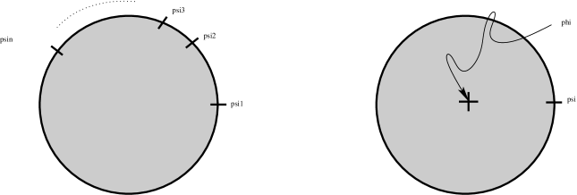
Figure 1: Left: The disk amplitude with $n+1$ boundary insertions captures the higher $A_{\infty}$ products (2.29). Right: The disk amplitude with one bulk and one boundary insertion encodes the bulk to boundary obstruction map (2.33), and will also define the infinitesimal Abel-Jacobi map (2.62).

Not only are open string deformations often obstructed by the non-vanishing of higher products on the ${\rm Ext}$-groups, but the very presence of background D-branes can sometimes obstruct the closed string deformations. Since this will be important later on, let us give a brief worldsheet derivation of this fact.

A basic feature of F-terms in supersymmetric theories is that they are supersymmetric only up to a total derivative. In spacetimes or on worldsheets with boundary therefore, this can lead to a non-vanishing boundary term in the supersymmetry variation. Consider in our framework the deformation of the bulk action as in (2.2). By using the topological descent relations

$$\{G^{+},\phi^{(2)}\}=\partial\phi^{(1)}\,,\qquad\{{\overline{G}}^{+},\phi^{(2)}\}=\bar{\partial}\phi^{(1)}$$ (2.31)

we see that its supersymmetry variation on a worldsheet, $\Sigma$, with non-empty boundary produces a boundary term,

$$\delta_{Q}(\delta S)=\int_{\Sigma}\{G^{+}+{\overline{G}}^{+},\phi^{(2)}\}=\int_{\Sigma}(\partial+\bar{\partial})\phi^{(1)}=\int_{\Sigma}d\phi^{(1)}=\int_{\partial\Sigma}\phi^{(1)}\quad\bigl{(}+{\it c.c.}\bigr{)}$$ (2.32)

In the context of topological field theories, the boundary term on the RHS of (2.32) has come to be known as “the Warner problem” [38].

By using (2.27), the boundary $U(1)$ charge of $\phi^{(1)}|_{\partial\Sigma}$ is $p=2$, and since it is still BRST closed, we obtain a well-defined open string chiral field from ${\cal H}^{2}_{\rm open}$. This defines the bulk-to-boundary obstruction map

$$m_{0}:TM\cong{\cal H}^{1,1}_{\rm closed}\to{\rm Ext}^{2}(B,B)\cong{\cal H}^{2}_{\rm open}$$ (2.33)

which as indicated fits as a zeroth order product into the $A_{\infty}$-framework. (An $m_{1}$ can be identified as the BRST operator itself.) Diagrammatically, $m_{0}$ composed with the open string topological metric can be defined as the disk correlator with one bulk and one boundary insertion, see Fig. 1.

The further fate of the Warner problem depends on whether $m_{0}(\phi)$ vanishes in cohomology or not. If it is zero, this means that there is an open string operator $\psi$ satisfying

$$\phi^{(1)}|_{\partial\Sigma}=\{G^{+}_{\rm bdry},\psi^{(1)}\}$$ (2.34)

where $G^{+}_{\rm bdry}$ is the boundary part of the supercharge. Hence by adding the boundary term

$$\delta S_{\rm bdry}=-\int_{\partial\Sigma}\psi^{(1)}$$ (2.35)

to the action, we can cancel the Warner term in the susy variation, and the brane deforms with the closed string background.

On the other hand, if $m_{0}(\phi)\neq 0\in{\rm Ext}^{2}(B,B)$, we will not be able to deform the brane linearly with the background. However, note that by Serre duality (or worldsheet CPT), ${\rm Ext}^{2}(B,B)\cong{\rm Ext}^{1}(B,B)$, and it can happen that $m_{0}(\phi)$ is in the image of a higher product $m_{n}$ for some $n$. In this case, by locking together an obstructed boundary deformation with the bulk deformation, we can still deform the brane with the closed string.

The basic example to keep in mind is when there is just one bulk deformation, $t$, and one boundary deformation, $u$. The superpotential is now a function of $u$ and $t$, where we can treat the latter as a parameter.

$${\cal W}={\cal W}(u;t)=\mu_{0}tu-\frac{\mu_{n}}{n+1}{u^{n+1}}+{\cal O}(u^{n+2})$$ (2.36)

where $\mu_{0}$ and $\mu_{n}$ are constants. If $\mu_{0},\mu_{n}\neq 0$, then for $t=0$, $u$ is obstructed at order $n$, while for small $t\neq 0$, there are $n$ vacua $u\sim t^{1/n}$, and $u$ is massive around each of them.

Let us bring this discussion to the point. If the D-brane has no marginal deformations, then the bulk-to-boundary obstruction map must be zero because ${\rm Ext}^{2}=0$. If there is a marginal deformation, and a non-trivial $m_{0}$, but the D-brane does not obstruct the bulk deformation, then $\mu_{n}$ must be non-zero for some smallest $n\geq 2$, and the marginal boundary direction is lifted by a small bulk deformation.

2.4 Closed string holomorphic anomaly

As we have mentioned, topologically twisted ${\cal N}=2$ SCFTs can be coupled to 2d (topological) gravity by identifying the supercharges and their conjugates with BRST operators and antighosts of a critical bosonic string in which the ghost and matter fields do not decouple. Indeed, the algebra (2.1) is all that is needed to define string amplitudes by integration over the moduli space of Riemann surfaces.

If ${\cal M}^{(g)}$ denotes the moduli space of Riemann surfaces of genus $g\geq 2$, and $\mu_{a}$, $a=1,\ldots,3g-3$ the Beltrami differentials, we define the topological string amplitude at genus $g$ by the formula,

$${{\cal F}}^{(g)}=\int_{{\cal M}^{(g)}}[dm]\;\bigl{\langle}\prod_{a=1}^{3g-3}\bigl{(}\int\mu_{a}G^{-}\bigr{)}\bigl{(}\int\mu_{\bar{a}}{\overline{G}}^{-}\bigr{)}\bigr{\rangle}_{\Sigma_{g}}$$ (2.37)

where $\mu_{a}G^{-}\equiv(\mu_{a})^{z}_{\;{\bar{z}}}G^{-}_{zz}$ denotes the contraction of the Beltrami’s with the antighosts, and $\langle\cdots\rangle_{\Sigma_{g}}$ the 2d field theory correlator on the worldsheet $\Sigma_{g}$. By this definition, the ${{\cal F}}^{(g)}$ become sections of the line bundle ${\cal L}^{2g-2}$ over the CFT moduli space $M$. The definition has to be modified slightly for $g=0$ and $g=1$ because of the presence of ghost zero modes as usual.

To derive the holomorphic anomaly equation, BCOV consider an infinitesimal deformation of the action by

$$t^{i}\int\phi_{i}^{(2)}+t^{\bar{i}}\int\phi_{\bar{i}}^{(2)}$$ (2.38)

and differentiate (2.37) with respect to $t^{\bar{i}}$. This leads to the insertion of $\int\phi_{\bar{i}}^{(2)}=\int d^{2}z\sqrt{h}\{G^{+},[{\overline{G}}^{+},\phi_{\bar{i}}]\}$ in the topological correlator. By contour deformation, one can move the action of the BRST operators to the Beltrami differentials folded with the anti-ghosts. By using the zero-mode algebra (2.1), the contractions are converted into differentials $\partial\langle\cdots\rangle$, $\bar{\partial}\langle\cdots\rangle$ on ${\cal M}^{(g)}$,

$$\frac{\partial}{\partial t^{\bar{i}}}{{\cal F}}^{(g)}=\int_{{\cal M}^{(g)}}[dm]\sum_{a,{\bar{a}}=1}^{3g-3}4\frac{\partial^{2}}{\partial m^{a}\partial m^{\bar{a}}}\bigl{\langle}\int\phi_{\bar{i}}\prod_{\genfrac{}{}{0.0pt}{2}{\scriptstyle a^{\prime}\neq a}{\scriptstyle{\bar{a}}^{\prime}\neq{\bar{a}}}}\bigl{(}\int\mu_{a^{\prime}}G^{-}\bigr{)}\bigl{(}\int\mu_{{\bar{a}}^{\prime}}{\overline{G}}^{-}\bigr{)}\bigr{\rangle}_{\Sigma_{g}}$$ (2.39)

Thus the anti-holomorphic derivative of ${{\cal F}}^{(g)}$ has been converted into the integral of a total derivative over ${\cal M}^{(g)}$. Naively, this is zero, but a careful analysis reveals that the correlator $\langle\int\phi_{\bar{i}}\cdots\rangle_{\Sigma_{g}}$ exhibits singularities around certain “boundary components” of ${\cal M}^{(g)}$, which correspond to our Riemann surface degenerating in various ways. Two types of degenerations are relevant for the closed string. The Riemann surface can split in two components by developing a long tube, or a handle can pinch without leading to a disconnected $\Sigma_{g}$. See fig. 2.

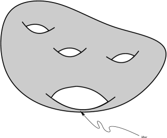
Figure 2: The two degenerations that contribute to the RHS of the holomorphic anomaly for closed strings.

In the derivation, one has to pay close attention to the location of the anti-chiral field in the limit where $\Sigma_{g}$ degenerates. As it turns out, the whole contribution comes from the region where $\phi_{\bar{i}}$ is sitting on the long tube. Thus, one is more nearly considering a Riemann surface which pinches at both ends of the tube. In the limit, the pinches are each repaired by inserting complete sets of chiral fields, $\phi_{j}$, $\phi_{k}$ on the lower-genus Riemann surface. The long tube is replaced with the three-point function on the sphere with insertion of anti-chiral fields, $\phi_{\bar{i}}$, $\phi_{\bar{j}}$, $\phi_{\bar{k}}$. This reduces to the anti-holomorphic Yukawa coupling $C_{{\bar{i}}{\bar{j}}{\bar{k}}}$. The connection between the various pieces of $\Sigma_{g}$ occurs via the inverse of the topological metric $g^{{\bar{j}}j}$, $g^{{\bar{k}}k}$.

Another important aspect of the derivation is that (for $g\geq 2$!), the sums at the location of the pinches are actually only over the marginal fields, i.e., those of charge $(q,{\bar{q}})=(1,1)$. This restriction arises from combining $U(1)$ charge conservation on the sphere, $q_{i}+q_{j}+q_{k}=3$, with the fact that $\phi_{a}^{(2)}=0$ for $q_{a}=0$. Namely, integrated insertion of the identity operator leads to a vanishing contribution. Since $q_{i}=1$ already, the only remaining possibility is $q_{j}=q_{k}=1$.

Taken together, one obtains the holomorphic anomaly equation for ${{\cal F}}^{(g)}$ ($g\geq 2$) as derived in BCOV

$$\partial_{\bar{i}}{{\cal F}}^{(g)}=\frac{1}{2}\sum_{g_{1}+g_{2}=g}C_{{\bar{i}}}^{jk}{{\cal F}}^{(g_{1})}_{j}{{\cal F}}^{(g_{2})}_{k}+\frac{1}{2}C_{{\bar{i}}}^{jk}{{\cal F}}^{(g-1)}_{jk}\,,$$ (2.40)

where the $\frac{1}{2}$ is a symmetry factor, and $C_{\bar{i}}^{jk}\equiv C_{{\bar{i}}{\bar{j}}{\bar{k}}}g^{{\bar{j}}j}g^{{\bar{k}}k}=C_{{\bar{i}}{\bar{j}}{\bar{k}}}{\it e}^{2K}G^{{\bar{j}}j}G^{{\bar{k}}k}$. The ${{\cal F}}^{(g)}$ with subscripts are the topological string amplitudes with insertion of the corresponding chiral fields, and are defined by

$${{\cal F}}^{(g)}_{i_{1},\ldots,i_{n}}=\int_{{\cal M}^{(g)}}[dm]\;\bigl{\langle}\int\phi_{i_{1}}^{(2)}\cdots\int\phi_{i_{n}}^{(2)}\prod_{a=1}^{3g-3}\bigl{(}\int\mu_{a}G^{-}\bigr{)}\bigl{(}\int\mu_{\bar{a}}{\overline{G}}^{-}\bigr{)}\bigr{\rangle}$$ (2.41)

As also shown in BCOV, the amplitudes with insertions can be obtained from the partition functions, ${{\cal F}}^{(g)}$, by covariant differentiation,

$${{\cal F}}^{(g)}_{i_{1},\ldots,i_{n+1}}=D_{i_{n+1}}{{\cal F}}^{(g)}_{i_{1},\ldots,i_{n}}$$ (2.42)

where again $D$ is the Zamolodchikov-Kähler covariant derivative on ${\rm Sym}^{n}T^{*}M\otimes{\cal L}^{2g-2}$.

Note that in (2.40), the sum is restricted to $g_{i}\geq 1$, which is a consequence of the vanishing of the sphere one and two-point function. Namely, we only encounter stable degenerations, with $3g_{i}-3+n_{i}>0$ for $i=1,2$, where $n_{i}\equiv 1$ is the number of marked points on the $i$-th component.

2.5 More on the vacuum bundle. D-branes as normal functions

Let us begin this subsection with a minor comment, which will gain some importance in the one-loop holomorphic anomaly in subsection 2.8. As we have recalled above, topological string amplitudes at genus $g$ are sections of the non-trivial line bundle ${\cal L}^{2g-2}$ over moduli space $M$. This arises because the ambiguity in normalizing the twisted path-integral on the worldsheet is determined by the choice of a canonical closed string vacuum $e_{0}=|0\rangle_{\rm closed}$. It is natural to ask whether the presence of boundaries could introduce new ambiguities, and lead to additional twisting. In fact, there are no new ambiguities, as can be seen from considering the topological path-integral on a disk with a long strip attached (Fig. 3). Given $|0\rangle_{\rm closed}$, this defines a canonical open string vacuum $|0\rangle_{\rm open}$, with a canonical normalization. As a consequence, open topological string amplitudes at genus $g$ with $h$ boundaries will be sections of ${\cal L}^{2g+h-2}$ over $M$.

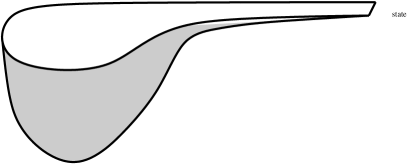
Figure 3: The path-integral on the disk with a long strip attached defines a canonical open string vacuum.

To continue the discussion, it will be helpful to have in mind a more concrete geometric realization of the topological string. So let us consider the B-model on a family of Calabi-Yau manifolds, all denoted by $Y$. The ground states are identified with the cohomology of $Y$ via

$${\cal H}^{p,q}\cong H^{3-p,q}(Y)$$ (2.43)

while the $(c,c)$-ring structure is determined from the identification

$$H^{3-p,q}(Y)\cong H^{q}(\Lambda^{p}TY)$$ (2.44)

given by contraction with the holomorphic 3-form, $\Omega$. The moduli space $M$ is the space of complex structure deformations of $Y$. As $Y$ varies over $M$, the middle dimensional cohomology groups $H^{3}(Y)$ fit together into a holomorphic vector bundle, which is precisely the vacuum bundle ${\cal V}$ we have discussed in subsection 2.2 above. The decomposition (2.9) is now

$${\cal V}_{m}=H^{3,0}(Y)\oplus H^{2,1}(Y)\oplus H^{1,2}(Y)\oplus H^{0,3}(Y)$$ (2.45)

An important point is that the decomposition (2.45) is not compatible with the holomorphic structure on ${\cal V}$. Instead, consider the Hodge filtration on $H^{3}(Y)$,

$$H^{3,0}(Y)=F^{3}H^{3}(Y)\subset F^{2}H^{3}(Y)\subset F^{1}H^{3}(Y)\subset F^{0}H^{3}(Y)=H^{3}(Y)$$ (2.46)

where

$$F^{q}H^{3}(Y)=\oplus_{q^{\prime}\geq q}H^{q^{\prime},3-q^{\prime}}(Y)$$ (2.47)

is the space of three-forms with at least $q$ holomorphic indices. The $F^{q}H^{3}(Y)$ do fit together into holomorphic subbundles of ${\cal V}$ over $M$. In particular, $F^{3}H^{3}(Y)=H^{3,0}(Y)$ is identified with our canonical line bundle ${\cal L}$.

The topological metric on ${\cal V}$ is up to a sign, $(-1)^{q}$, the symplectic pairing between $H^{3-q,q}(Y)$ and $H^{q,3-q}(Y)$, while the Zamolodchikov metric is identified with the Weil-Petersson metric on $M$

$$G_{i{\bar{j}}}=\partial_{i}\partial_{\bar{j}}K\,,\qquad\text{where }\;K=-\log{\it i}\int_{Y}{\overline{\Omega}}\wedge\Omega$$ (2.48)

The structure constants of the chiral ring are given by

$$C_{ijk}=-\int_{Y}\Omega\wedge\partial_{i}\partial_{j}\partial_{k}\Omega$$ (2.49)

The vacuum bundle ${\cal V}$ comes equipped with a real structure, which is induced from the embedding $H^{3}(Y;{\mathbb{R}})\subset H^{3}(Y;{\mathbb{C}})$. Complex conjugation acts by exchanging $H^{q,3-q}$ with $H^{3-q,q}$ and corresponds on the worldsheet to the CPT operator $\Theta$.

It can hardly be overemphasized that the starting point for much of special geometry and in fact the entire story of the holomorphic anomaly is the competition between the holomorphicity of the filtration (2.46), which would make topological string amplitudes holomorphic, and the reality of the decomposition (2.45), which is preferred for maintaining unitarity of the worldsheet CFT. We will see that this is crucial when we add boundaries as well.

Not only do we have a real structure on $H^{3}(Y;{\mathbb{C}})\supset H^{3}(Y;{\mathbb{R}})$, but we also have an integral structure from the embedding $H^{3}(Y;{\mathbb{Z}})\subset H^{3}(Y;{\mathbb{R}})$. The Gauss-Manin connection on $H^{3}(Y;{\mathbb{C}})$ can be characterized by the fact that it preserves this integral structure. Namely, any section of $H^{3}(Y;{\mathbb{Z}})$ is flat with respect to the Gauss-Manin connection. On the Hodge filtration, the Gauss-Manin connection satisfies Griffiths transversality

$$\nabla F^{q}H^{3}(Y)\subset F^{q-1}H^{3}(Y)$$ (2.50)

If $\Gamma\in H_{3}(Y;{\mathbb{Z}})$ is an integral 3-cycle, it defines an element in $H^{3}(Y;{\mathbb{Z}})$ by integration against 3-forms and duality. Of importance are the periods of the holomorphic three-form

$$\Pi(z)=\langle\phi_{0},\Gamma\rangle=\int_{\Gamma}\Omega(z)$$ (2.51)

where $z=(z^{i})_{i=1,\ldots,n}$ is some collection of local coordinates on $M$. The pairings with the $(2,1)$-forms $\chi_{i}$ can be obtained by differentiation,

$$D_{i}\Pi(z)=\partial_{i}\Pi(z)+\partial_{i}K\Pi(z)=\langle\phi_{i},\Gamma\rangle=\int_{\Gamma}\chi_{i}^{(2,1)}(z)$$ (2.52)

while the overlaps with the $(1,2)$ and $(0,3)$-forms follow (for instance) by complex conjugation.

It will be useful for us to introduce at this stage the so-called Griffiths intermediate Jacobian. At any point in moduli space, we consider the complex torus

$$J^{3}(Y)=H^{1,2}(Y)\oplus H^{0,3}(Y)/H^{3}(Y;{\mathbb{Z}})=H^{3}(Y;{\mathbb{C}})/(F^{2}H^{3}(Y)+H^{3}(Y;{\mathbb{Z}}))$$ (2.53)

(The underlying real torus is $H^{3}(Y;{\mathbb{R}})/H^{3}(Y;{\mathbb{Z}})$, the complex structure is determined by the complex structure on $Y$.) Because of the holomorphicity of the filtration (2.46), the $J^{3}(Y)$ fit together into a holomorphic family of complex tori, known as the intermediate Jacobian fibration.

We can now begin to ask more precisely how D-branes fit into the framework of special geometry and the vacuum bundle over $M$. A-branes first.

From the worldsheet perspective, A-branes are essential to define the integral structure on the vacuum bundle. Indeed, while the worldsheet CPT operator defines the real structure, it does not allow the selection of an integral lattice inside of it. But consider two A-branes $A$ and $A^{\prime}$. By general principles, we can express the Witten index in the Hilbert space of $A$–$A^{\prime}$-strings via the overlaps of the boundary states with the Ramond ground states, which for A-branes must be taken from the B-model as we have explained in subsection 2.3

$${\rm tr}_{A-A^{\prime}}(-1)^{F}=\langle A|e_{a}\rangle\eta^{ab}\langle e_{b}|A^{\prime}\rangle$$ (2.54)

where $e_{a}$ is some basis of ${\cal V}$, and $\eta^{ab}$ the inverse topological metric. Geometrically, A-branes wrap (special) Lagrangian three-cycles in $Y$. Their class in $H_{3}(Y;{\mathbb{Z}})$ defines the overlap with ${\cal V}$ via (2.51), (2.52), and their (integral!) intersection number computes the Witten index (2.54). Thus, properly normalized A-brane boundary states define integral sections of ${\cal V}$.

B-branes are more subtle. (Useful references for the geometric statements that will follow below include [39, 40].) As we have mentioned before, the modern perspective is that D-branes are mathematically well accommodated in certain categories endowed with extra structure, such as the $A_{\infty}$-structure we have discussed in subsection 2.3. For our B-model on $Y$, the relevant category is the bounded derived category of coherent sheaves, $D^{b}(Y)$. Essentially, this includes D-branes wrapped on even-dimensional, holomorphic cycles carrying holomorphic vector bundles, as well as all possible “topological bound states” of those that can be obtained by “topological tachyon condensation”.

Our main goal is to extract holomorphic information from objects in the B-brane category, and to relate it to the vacuum bundle ${\cal V}$. It is in any case clear already that the topological classification of B-branes involves ground states from the other model, which are not contained in ${\cal V}$. For reasons that will become completely clear only in subsection 2.7, we want to restrict ourselves to B-branes whose overlaps with those ground states with $q_{\it rgs}=-{\bar{q}}_{\it rgs}$ vanish. The point is that if those overlaps don’t vanish, one is in danger that the corresponding A-model deformations, which are BRST exact in the B-model, will not decouple in loop computations. For this reason, and because it seems plausible that analogous effects can be achieved by (topological) orientifolds, we refer to this condition as “tadpole cancellation”.

Physically, all the holomorphic information one expects to extract from the open string at tree-level is captured in the spacetime superpotential ${\cal W}$ for the massless fields on the brane. The interpretation of the superpotential in $A_{\infty}$-categories is quite well understood, but depends to a large extent on gauge-fixing data of the open string field theory [41, 37]. Gauge invariant physical information contained in the superpotential is for example the tension of BPS domainwalls, ${\cal T}=\Delta{\cal W}$. Since such domainwalls carry no topological D-brane charge, they are precisely the physical objects satisfying the tadpole cancellation condition from the previous paragraph. We will henceforth restrict ourselves to such configurations.

Consider for instance wrapping of a D5-brane on a holomorphic curve $C\subset Y$. This B-brane carries no topological charge if its class in $H_{2}(Y;{\mathbb{Z}})$ vanishes. It can then arise as a domainwall between two D5-branes wrapped on two different holomorphic curves $C_{+}$ and $C_{-}$ in the same class if $C=C_{+}-C_{-}$ holomorphically. The tension of the BPS domainwall is [42]

$${\cal T}=\int_{\Gamma}\Omega$$ (2.55)

where $\Omega(z)$ is the holomorphic three-form and $\Gamma$ is a three-chain in $Y$ with boundary $\partial\Gamma=C=C_{+}-C_{-}$. The domainwall tension depends on complex structure moduli both explicitly through the holomorphic three-form, as well as implicitly through the position of the curve $C$, which must vary in order to remain holomorphic as we vary the complex structure. At this stage, we also allow dependence of ${\cal T}$ on any moduli of $C$ for fixed complex structure of $Y$, but we will drop this freedom in the next subsection.

Because the holomorphic three-form is unique up to scale, formula (2.55) is well-defined even if we think of $\Omega$ just as a representative of a cohomology class in $H^{3,0}(Y)$. Because $\Gamma$ has a boundary, we could not integrate an arbitrary cohomology class over it. However, next to $\Omega$, we can do one more. Consider a class $[\chi^{(2,1)}]$ in $H^{2,1}(Y)$. It is an elementary fact from Hodge theory that $F^{p}H^{k}\cong(F^{p}A^{k})^{c}/dF^{p}A^{k-1}$, where $F^{p}A^{k}$ are the $k$-forms on $Y$ with at least $p$ holomorphic indices, $(\cdot)^{c}$ refers to closed forms, and $d$ is the total differential. Thus we can represent $[\chi^{2,1}]$ by a closed form $\chi^{(2,1)}\in F^{2}A^{3}$ and define the integral

$$\int_{\Gamma}\chi^{(2,1)}$$ (2.56)

The integral does not depend on the choice of representative since under $\chi^{(2,1)}\to\chi^{(2,1)}+d\xi^{(2,0)}$, where $\xi^{(2,0)}$ is a $(2,0)$-form, the integral changes by $\int_{\partial\Gamma}\xi^{(2,0)}$, and since $\partial\Gamma=C$ is a holomorphic curve, the integral of a $(2,0)$-form over it vanishes.

The properties we have just described are part of the definition of a Poincaré normal function, in the sense of Griffiths [13] (see [39] for a pedagogical introduction). Formally, a normal function $\nu$ is a holomorphic section of the intermediate Jacobian (2.53) satisfying the infinitesimal condition for normal functions, or Griffiths transversality, defined as follows. If $\nu$ is any holomorphic section of $J^{3}(Y)=H^{3}(Y)/(F^{2}H^{3}+H^{3}({\mathbb{Z}}))$, one can choose a lift of $\nu$ as a holomorphic section $\tilde{\nu}$ of $H^{3}(Y)$. Then we can apply the Gauss-Manin connection $\nabla$ to $\tilde{\nu}$, and Griffiths transversality for normal functions is the statement

$$\nabla\tilde{\nu}\in F^{1}H^{3}$$ (2.57)

Instead of showing that this condition is independent of the lift (which it is), let us verify that a family of holomorphic curves indeed defines a normal function. Note that by duality, we can identify $H^{3}/F^{2}H^{3}$ with $(F^{2}H^{3})^{*}$ and $J^{3}(Y)$ with $(F^{2}H^{3})^{*}/H_{3}(Y;{\mathbb{Z}})$. Correspondingly, the integrals (2.55), (2.56) define an element of $(F^{2}H^{3})^{*}=(H^{3,0}\oplus H^{2,1})^{*}$, and the three-chain $\Gamma$ with $\partial\Gamma=C$ is only defined up to a three-cycle in $H_{3}(Y;{\mathbb{Z}})$. Thus, $C$ defines a section of the intermediate Jacobian. Finally, Griffiths transversality (2.57) follows from the observation that when we vary the complex structure of $Y$, we can describe the first order variation of $C$ by a normal vector $n\in N_{C/Y}$. If $\delta\Gamma$ is the corresponding first order variation of $\Gamma$, one has

$$\int_{\delta\Gamma}\Omega=\int_{C}\Omega(n)=0$$ (2.58)

which again vanishes by type considerations since $C$ is holomorphic. This is equivalent to $\langle\Omega,\nabla\tilde{\nu}\rangle=0$, and hence to (2.57).

Normal functions also make sense for holomorphic vector bundles, and by splitting distinguished triangles can be defined for the entire derived category $D^{b}(Y)$. The essential device that makes this possible is the notion of algebraic or holomorphic second Chern class. Given for example a holomorphic vector bundle, we can equip it with a hermitian metric, and thus specify a connection, $A$, whose curvature $F=dA+A\wedge A$ is of type $(1,1)$. The second Chern form is $c_{2}(A)={\rm tr}F\wedge F$ and defines a cohomology class in $H^{4}(Y;{\mathbb{Z}})$. If $[c_{2}(A)]=0$, one may write $c_{2}(A)=d{\it CS}(A)$, where ${\it CS}(A)$ is the Chern-Simons form. This way, we identify the domainwall tension with Witten’s holomorphic Chern-Simons functional [43, 41, 44],

$${\cal T}=\int{\it CS}(A)\wedge\Omega$$ (2.59)

and indeed one can show that it depends only on the holomorphic class of the vector bundle.

Further details on the relation of D-branes to normal functions, with an important example, appear in [6].

2.6 Infinitesimal invariant and holomorphic anomaly on the disk

We have just seen that topologically trivial B-branes are holomorphically captured by a normal function, namely a holomorphic section of the intermediate Jacobian (2.53) satisfying Griffiths transversality (2.57). This association is known as the Abel-Jacobi map. It is worthwhile pointing out that in general, one can also consider intermediate Jacobians for 0-cycles, $J^{1}(Y)$, and for four-cycles, $J^{5}(Y)$. However, if $Y$ is simply connected (which we assume), those Jacobians, known as the Albanese and Picard variety, respectively, vanish. The Abel-Jacobi map was first used used for open string disk instanton computations (on non-compact Calabi-Yau) by Aganagic and Vafa [45]. Early speculations on the relevance of the Abel-Jacobi map to mirror symmetry appear in [46]. In this subsection, we study the relation between the Abel-Jacobi map for B-branes and the vacuum bundle ${\cal V}$, especially at the infinitesimal level.

It is clear from the previous subsection that a normal function in itself cannot completely describe the topological boundary state of a B-brane. Granting a lift of the $H^{3}(Y;{\mathbb{Z}})$ ambiguity, $\nu$ only defines the $(0,3)$ and $(1,2)$ components of an element of $H^{3}(Y)$, and this only in the quotient. To get an actual state in ${\cal V}$, we need a lift $\tilde{\nu}$.

A little thought reveals that there is in fact a very natural lift of $\nu$ to all of ${\cal V}$, dictated by worldsheet CPT invariance. Since the latter is simply complex conjugation acting on $H^{3}(Y)$, we see that at the level of the pairing $\langle\Omega,\nu\rangle=\int_{\Gamma}\Omega$, (2.55), we are defining the lift by

$$\langle{\overline{\Omega}},\tilde{\nu}\rangle=\int_{\Gamma}{\overline{\Omega}}=\overline{\int_{\Gamma}\Omega}=\overline{\langle\Omega,\tilde{\nu}\rangle}$$ (2.60)

and similarly for the $(1,2)$-forms. We will henceforth denote this real lift of the normal function also by $\nu$.

Before studying the full consequences of this identification, let us finally clarify our intent to neglect open string moduli that has been lingering since (F1) in the introduction. We have seen already in subsection 2.3 that if bulk deformations are unobstructed by the D-brane and the obstruction map $m_{0}$ is non-zero, we can remove open string moduli by a small bulk deformation.

To deal with the assumption that $m_{0}$ is non-trivial, consider a family of homologically trivial B-branes $B(w)$, which as a function of some local parameter $w$ are all holomorphic with a fixed complex structure of $Y$. We can define the Abel-Jacobi map ${\it AJ}(w)\in J^{3}(Y)$. By considerations similar to those around (2.58), one can show that the first order variation of ${\it AJ}(w)$ satisfies

$$d_{w}{\it AJ}(w)\in F^{1}H^{3}(Y)/F^{2}H^{3}(Y)\cong H^{1,2}(Y)$$ (2.61)

This is similar to (2.57), except that we now vary only the brane for fixed complex structure of $Y$. Since the tangent space to moduli of $B(w)$ is ${\rm Ext}^{1}(B,B)$ as reviewed in subsection 2.3, the infinitesimal Abel-Jacobi map is more abstractly a map

$$\alpha:{\rm Ext}^{1}(B,B)={\cal H}^{1}_{\rm open}\to H^{1,2}(Y)={\cal H}^{2,2}_{\rm closed}$$ (2.62)

Diagrammatically, by using the closed string topological metric, we can identify $\alpha$ with the two point function on the disk with one boundary and one bulk insertion, see Fig. 1. Referring back to subsection 2.3, we see that the infinitesimal Abel-Jacobi map is nothing but the dual of the bulk-to-boundary obstruction map (2.33), $\alpha=m_{0}^{*}$. Thus, if $m_{0}$ vanishes, the image of $B(w)$ in the intermediate Jacobian is independent of $w$, and, if the brane does not obstruct the bulk, the corresponding normal function will also not depend on $w$.

When the B-brane is a holomorphic vector bundle, these statements are reflected in the fact that the holomorphic Chern-Simons functional (2.59) is constant on unobstructed families of holomorphic connections [44]. In fact, the holomorphic Chern-Simons functional (or, more generally, the open string field theory) and its quantization encodes the entire deformation and obstruction theory for B-branes [47]. We are here only concerned with its most elementary application.

An extremely useful concept attached to normal functions in the context of infinitesimal variation of Hodge structure is the so-called Griffiths’ infinitesimal invariant. It was first considered by Griffiths in [14], and later refined by Voisin [15] and Green [16]. If one insists on holomorphicity, defining the infinitesimal invariant requires some ingenuity, because one cannot quite do it without choosing a lift of $\nu$ to $H^{3}(Y)$ (see [39]). But since we have given up on holomorphicity long ago, and work with the real physical lift (2.60), we can be more pedestrian. Our main goal is to explain the identification of the infinitesimal invariant with the disk two-point function, see (F3) in the introduction.

Consider a real normal function $\nu$, and expand in a basis of the vacuum bundle, see eq. (2.13),

$$\nu=\nu^{0}e_{0}+\nu^{i}e_{i}+\nu^{\bar{i}}e_{\bar{i}}+\nu^{\bar{0}}e_{\bar{0}}$$ (2.63)

where reality means $\nu^{\bar{i}}=\overline{\nu^{i}}$, $\nu^{\bar{0}}=\overline{\nu^{0}}$. The domainwall tension is of course ${\cal T}=\langle\Omega,\nu\rangle=\langle e_{0},\nu\rangle=\nu^{\bar{0}}g_{0{\bar{0}}}$. By utilizing the explicit form of the connection matrices in subsection 2.2, we find

$$\nabla_{i}\nu=(\partial_{i}\nu^{0}-\partial_{i}K\nu^{0})e_{0}+\bigl{(}\partial_{i}\nu^{l}+g^{{\bar{k}}l}\partial_{i}g_{m{\bar{k}}}\nu^{m}-\delta_{i}^{l}\nu^{0}\bigr{)}e_{l}+\\ \bigl{(}\partial_{i}\nu^{\bar{l}}-C_{im}^{\;\;\;\;{\bar{l}}}\nu^{m}\bigr{)}e_{\bar{l}}+\bigl{(}\partial_{i}\nu^{\bar{0}}-G_{i{\bar{m}}}\nu^{\bar{m}}\bigr{)}e_{\bar{0}}$$ (2.64)

Griffiths transversality for normal functions is the statement $\langle\Omega,\nabla\nu\rangle=0$, which translates into

$$D_{i}{\cal T}=\partial_{i}{\cal T}+\partial_{i}K{\cal T}=\nu_{i}=g_{i{\bar{j}}}\nu^{\bar{j}}$$ (2.65)

The Griffiths’ infinitesimal invariant can now be defined as the following tensor in $(T^{*}M)^{2}\otimes{\cal L}^{-1}$,

$$\Delta_{ij}:=-\langle\nabla_{i}\Omega,\nabla_{j}\nu\rangle$$ (2.66)

By using Griffiths transversality and the compatibility of the Gauss-Manin connection with the symplectic metric, this is equivalent to

$$\Delta_{ij}=\langle\Omega,\nabla_{i}\nabla_{j}\nu\rangle$$ (2.67)

which makes it obvious that $\Delta_{ij}$ is symmetric in $i$ and $j$, i.e., $\Delta_{ij}\in{\rm Sym}^{2}(T^{*}M)\otimes{\cal L}^{-1}$. From (2.64), we find explicitly

$$\Delta_{ij}=D_{i}D_{j}{\cal T}-C_{ijk}g^{{\bar{k}}k}D_{\bar{k}}\overline{\cal T}$$ (2.68)

From the definition, it is clear that $\Delta_{ij}$ vanishes identically if ${\cal T}$ is a period of the holomorphic three-form over a (closed) three-cycle. To verify this, one has to be careful to insert an actual real period, and not just an arbitrary complex solution of the Picard-Fuchs equation. These notions are not equivalent since (2.68) is not holomorphic in ${\cal T}$. But in any event, we see that the infinitesimal invariant does not depend on how we choose to lift the $H^{3}(Y;{\mathbb{Z}})$ ambiguity in the definition of the normal function. It is also invariant under monodromies in the complex structure moduli space, for the same reason.

To show the identification of $\Delta_{ij}$ with the disk two-point function, we will make use of the holomorphic anomaly. From (2.68) and the special geometry relations, it is not hard to see that our infinitesimal invariant satisfies the distinctive equation

$$\partial_{\bar{i}}\Delta_{jk}=-C_{jkl}g^{{\bar{l}}l}D_{\bar{i}}D_{\bar{l}}\overline{{\cal T}}+C_{jkl}C_{{\bar{i}}{\bar{l}}{\bar{m}}}g^{{\bar{l}}l}g^{{\bar{m}}m}D_{m}{\cal T}=-C_{jkl}g^{{\bar{l}}l}\Delta_{{\bar{i}}{\bar{l}}}$$ (2.69)

where $\Delta_{{\bar{k}}{\bar{l}}}=\overline{\Delta_{kl}}$.

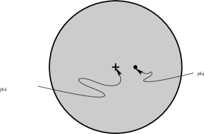
Figure 4: The disk amplitude with two bulk insertions.

On the other hand, the topological string amplitude on the disk with two bulk insertions is defined by

$$\tilde{\Delta}_{jk}=\int_{0}^{1}dr\langle\phi_{j}(0)\phi_{k}^{[1]}(r)\rangle_{(0,1)}$$ (2.70)

where one of the insertions is fixed at $0$, and we are integrating over the radial position of the one-form descendant $\phi_{k}^{[1]}=\frac{1}{2}[G^{-}-{\overline{G}}^{-},\phi_{k}]$ of the other. Taking a derivative of $\tilde{\Delta}_{jk}$ in the anti-holomorphic direction brings down the anti-chiral insertion $\int\phi_{\bar{i}}^{(2)}=\int d^{2}z\sqrt{h}\frac{1}{2}\{G^{+}+{\overline{G}}^{+},[G^{+}-{\overline{G}}^{+},\phi_{\bar{i}}]\}$. This is BRST exact in the presence of the boundary, and similarly to the derivation in subsection 2.4, we can move the BRST operator to the chiral insertion, where $\{G^{+}+{\overline{G}}^{+},\phi_{k}^{[1]}\}=d\phi_{k}$. Thus we are reduced to

$$\partial_{\bar{i}}\tilde{\Delta}_{jk}=\int_{0}^{1}dr\frac{\partial}{\partial r}\langle\int\phi_{\bar{i}}^{[1]}\phi_{j}(0)\phi_{k}(r)\rangle_{(0,1)}$$ (2.71)

where $\phi_{\bar{i}}^{[1]}=\frac{1}{2}[G^{+}-{\overline{G}}^{+},\phi_{\bar{i}}]$. This is now a sum of two boundary terms. When $\phi_{k}$ hits the boundary at $r=1$, we obtain a term similar to the Warner term in the supersymmetry variation of the bulk action (2.32). By our assumptions, the Warner term has been canceled as in (2.34), in other words $\phi_{k}|_{\partial\Sigma}$ is BRST exact on the boundary. So there is no contribution from $r=1$. On the other hand, the boundary term at $r=0$, when $\phi_{j}$ and $\phi_{k}$ collide, can be evaluated by using the bulk chiral ring and $tt^{*}$-fusion. Thus,

$$\partial_{\bar{i}}\tilde{\Delta}_{jk}=-C_{jkl}g^{{\bar{l}}l}\int_{0}^{1}dr\langle\phi_{\bar{l}}(0)\phi_{\bar{i}}^{[1]}(r)\rangle_{(0,1)}=-C_{jkl}g^{{\bar{l}}l}\tilde{\Delta}_{{\bar{i}}{\bar{l}}}$$ (2.72)

where we have made use of the fact that the angular integration of $\phi_{\bar{i}}^{[1]}$ is trivial once $\phi_{j}$ and $\phi_{k}$ have been fused. This shows that $\tilde{\Delta}_{ij}$ satisfies exactly the same holomorphic anomaly equation as $\Delta_{ij}$. Modulo the holomorphic ambiguity, this completes our identification of the two-point function on the disk with the non-holomorphically lifted Griffiths infinitesimal invariant of the normal function. We believe that this identification also holds after the holomorphic ambiguity has been taken into account. We will be able to verify this in the example from independent information in the A-model.

We now have all the machinery in place to extend the holomorphic anomaly to higher worldsheet topologies.

2.7 Holomorphic anomaly with D-branes

In analogy to (2.37), we want to define the open topological amplitude ${{\cal F}}^{(g,h)}$ by an integral over the moduli space ${\cal M}^{(g,h)}$ of Riemann surfaces with genus $g$ and $h$ boundary components. In this subsection, let us assume $2g+h-2>0$. (We have discussed the disk amplitude in the previous subsection, and will return to the annulus amplitude in the next.) Given such a Riemann surface $\Sigma_{g,h}$, we can close off all the boundaries by gluing in a standard centered disk at each boundary component. The data one is forgetting is the length of the boundary component. This describes ${\cal M}^{(g,h)}$ as a fibration over ${\cal M}^{(g)}_{h}$, the moduli space of Riemann surfaces of genus $g$ with $h$ marked points

$$\bigl{(}{\mathbb{R}}^{+}\bigr{)}^{h}\to{\cal M}^{(g,h)}\to{\cal M}^{(g)}_{h}$$ (2.73)

Consequentially, when thinking about the infinitesimal variations of $\Sigma_{g,h}$, we can isolate those which only change the lengths of the boundary components, from those which affect also the bulk of the Riemann surface. We introduce the (real) length moduli by $l^{b}$, and the coordinates on ${\cal M}^{(g)}_{h}$ by $m^{a}$. Let us also denote the Beltrami differentials pulled back from ${\cal M}^{(g)}_{h}$ by $\mu_{a},\mu_{\bar{a}}$, $a,{\bar{a}}=1,\ldots 3g+h-3$, and the other ones by $\lambda_{b}$, $b=1,\ldots h$.

We now define the topological string amplitude ${{\cal F}}^{(g,h)}$ by

$${{\cal F}}^{(g,h)}=\int_{{\cal M}^{(g,h)}}[dm][dl]\;\bigl{\langle}\prod_{a=1}^{3g+h-3}\bigl{(}\int\mu_{a}G^{-}\bigr{)}\bigl{(}\int{\bar{\mu}}_{\bar{a}}{\overline{G}}^{-}\bigr{)}\prod_{b=1}^{h}\lambda_{b}(G^{-}+{\overline{G}}^{-})\bigr{\rangle}_{\Sigma_{g,h}}$$ (2.74)

It is important here that the $\mu_{a}$ are complex and can be localized away from the boundary $\partial\Sigma_{g,h}$. It therefore makes sense to contract them with the $G^{-},{\overline{G}}^{-}$ individually. On the other hand, the $\lambda_{b}$ are real, and supported near $\partial\Sigma_{g,h}$. So we need to contract them with the combination that is preserved at the boundary, $G^{-}+{\overline{G}}^{-}$.

The ${{\cal F}}^{(g,h)}$ are sections of ${\cal L}^{2g+h-2}$ over $M$. Recall that we assume all closed string deformations to be unobstructed by the branes, and do not consider any other independent open string moduli, so $M$ is the same as before. Also as before, taking a derivative with respect to the anti-holomorphic parameter $t^{\bar{i}}$ brings down the BRST trivial operator $\int\phi_{\bar{i}}^{(2)}=\int d^{2}z\sqrt{h}\{G^{+},[{\overline{G}}^{+},\phi_{\bar{i}}]\}$ into the correlator.

When we now pull the action of the BRST operator to the anti-ghosts, we have to distinguish whether we hit the complex Beltramis from ${\cal M}^{(g)}_{h}$ or the real ones corresponding to the variation of the lengths of the boundary components. In the latter case, we can only contract with the BRST charge that is preserved at the boundary, and remain with an insertion of $\phi_{\bar{i}}^{[1]}\equiv\frac{1}{2}[G^{+}-{\overline{G}}^{+},\phi_{\bar{i}}]$ in the correlator [2]. Thus, we obtain

$$\begin{split}\partial_{\bar{i}}{{\cal F}}^{(g,h)}&=\int_{{\cal M}^{(g,h)}}[dm][dl]\Biggl{[}\;\sum_{a,{\bar{a}}=1}^{3g+h-3}4\frac{\partial^{2}}{\partial m^{a}\partial m^{\bar{a}}}\bigl{\langle}\int\phi_{\bar{i}}\prod_{\genfrac{}{}{0.0pt}{2}{\scriptstyle a^{\prime}\neq a}{\scriptstyle{\bar{a}}^{\prime}\neq{\bar{a}}}}\bigl{(}\int\mu_{a^{\prime}}G^{-}\bigr{)}\bigl{(}\int\mu_{{\bar{a}}^{\prime}}{\overline{G}}^{-}\bigr{)}\\[-5.69046pt] &\qquad\qquad\qquad\qquad\qquad\qquad\qquad\qquad\qquad\qquad\prod_{b=1}^{h}\lambda_{b}(G^{-}+{\overline{G}}^{-})\bigr{\rangle}_{\Sigma_{g,h}}+\\ &\qquad\sum_{b=1}^{h}2\frac{d}{dl^{b}}\bigl{\langle}\int\phi_{\bar{i}}^{[1]}\prod_{a=1}^{3g+h-3}\bigl{(}\int\mu_{a}G^{-}\bigr{)}\bigl{(}\int{\bar{\mu}}_{\bar{a}}{\overline{G}}^{-}\bigr{)}\prod_{b^{\prime}\neq b}\lambda_{b^{\prime}}(G^{-}+{\overline{G}}^{-})\bigr{\rangle}_{\Sigma_{g,h}}\Biggr{]}\end{split}$$ (2.75)

(Strictly speaking, there are also terms which mix the base and the fiber directions of ${\cal M}^{(g,h)}$, but those can be shown to lead to a vanishing boundary contribution. The arguments are similar to those at the end of section 3.1 of BCOV.)

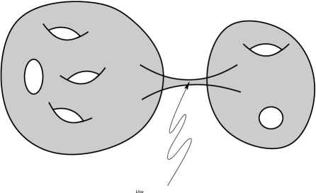
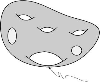
Figure 5: When adding boundaries, the two degenerations from Fig. 2 remain unaffected.

Now we have to analyze the contribution from the boundary of ${\cal M}^{(g,h)}$. As could be expected, the closed string degenerations familiar from subsection 2.4 remain essentially unaffected, see Fig. 5. The only difference is that when we split the Riemann surface in two pieces, we have to keep track of the distribution of the various components of $\partial\Sigma_{g,h}$. This leads to a sum over $(g_{1},h_{1})$, $(g_{2},h_{2})$ with $g_{1}+g_{2}=g$, $h_{1}+h_{2}=h$. The condition to have a stable degeneration imposes the additional restriction that $3g_{i}+3h_{i}/2-2>0$ for $i=1,2$, but in particular allows $g_{i}=0$ as long as $h_{i}\geq 2$.

There are three types of degenerations which are specific to the presence of open strings. The first two arise when the Riemann surface develops a very long strip, which can either split the Riemann surface in two pieces, or lead to the merging of two boundary components. It is not hard to see that those degenerations actually do not contribute. The presence of the very long strip projects the intermediate open strings to their ground states, and we can therefore replace the strip by the insertion of complete sets of chiral boundary fields, $\psi_{a}$ $\psi_{b}$, contracted with the open string topological metric $\eta^{ab}$. But notice that when $2g+h-2>0$, at least one of the boundary fields has to be an integrated insertion, and as in the closed string case, the only contribution could have come from marginal ($p=1$) open string states. Since those are generically absent, we conclude that degenerations with long strips do not contribute.

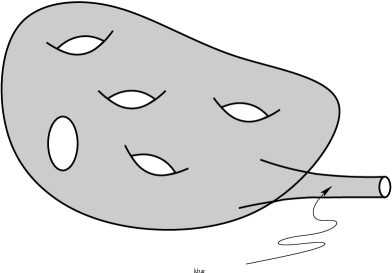
Figure 6: The degeneration with an intermediate open string does not contribute generically. This leaves only the degeneration in which the length of a boundary component shrinks to zero size, or, equivalently, the boundary component is separated by a long tube.

The final degeneration we have to take into account arises when the length of a boundary components shrinks to zero, i.e., $l^{b}\to 0$ in (2.75), see Fig. 6. This is conformally equivalent to pulling the boundary very far from the rest of the Riemann surface via a long tube, at which point it looks more like a closed string degeneration of the type we have seen before. Strictly speaking, however, it would not make sense to pinch off the tube because this would have corresponded to a non-stable degeneration (in real codimension 2!) involving a disk one-point function. Complementarily, we note that as long as the integration of the anti-chiral field $\phi_{\bar{i}}^{[1]}$ is away from the long tube, the intermediate closed string is projected onto the ground states. As explained in the previous subsection, our construction is such that all these one-point functions vanish (by tadpole cancellation or Griffiths transversality).

Thus, we only remain with the integration of $\phi_{\bar{i}}^{[1]}$ over the long tube. Note that the angular position of $\phi_{\bar{i}}^{[1]}$ does not matter after we pull the tube infinitely long. The infinitely long tube projects the closed string onto their ground states which can again be represented by inserting a complete set of chiral fields (only marginal ones contributing). So the rest of the Riemann surface has an additional chiral insertion of $\phi_{j}$, while the long tube becomes nothing but the anti-topological disk two-point function,

$$\Delta_{{\bar{i}}{\bar{j}}}=\int_{0}^{1}\langle\phi_{\bar{i}}^{[1]}(r)\phi_{\bar{j}}(0)\rangle_{0,1}\,,$$ (2.76)

familiar from the previous subsection. The connection to the bulk of the Riemann surface occurs via the inverse topological metric $g^{{\bar{j}}j}$. This way, we arrive at our final expression for the holomorphic anomaly equation in the presence of D-branes,

$$\partial_{\bar{i}}{{\cal F}}^{(g,h)}=\frac{1}{2}\sum_{\genfrac{}{}{0.0pt}{2}{\scriptstyle g_{1}+g_{2}=g}{\scriptstyle h_{1}+h_{2}=h}}C_{{\bar{i}}}^{jk}{{\cal F}}^{(g_{1},h_{1})}_{j}{{\cal F}}^{(g_{2},h_{2})}_{k}+\frac{1}{2}C_{{\bar{i}}}^{jk}{{\cal F}}^{(g-1,h)}_{jk}-\Delta_{{\bar{i}}}^{j}{{\cal F}}^{(g,h-1)}_{j}\,,$$ (2.77)

where we have of course defined

$$\Delta_{{\bar{i}}}^{j}\equiv\Delta_{{\bar{i}}{\bar{j}}}g^{{\bar{j}}j}=\Delta_{{\bar{i}}{\bar{j}}}{\it e}^{K}G^{{\bar{j}}j}$$ (2.78)

and the ${{\cal F}}^{(g,h)}$ with subscripts are the amplitudes with closed string insertions as before.

We call eq. (2.77) the “extended holomorphic anomaly equation”. It would be very interesting to clarify in greater detail the role played by marginal open string operators in this equation. As we have mentioned, it seems reasonable to expect that actual open string moduli do not enter the ${{\cal F}}^{(g,h)}$ at all. Massless open string fields with a higher order superpotential however will lead to additional singularities at isolated points in the moduli space, as we will see in examples in the second half of the paper. But before that, let us conclude this first half by tying up a few loose ends concerning the extended holomorphic anomaly.

2.8 Holomorphic anomaly at one loop

In our derivation so far, we have factored out the one-loop amplitudes, on the torus and the annulus for closed and open strings, respectively. These amplitudes are somewhat exceptional, because information enters which is slightly external to the B-model proper. Nevertheless, they fit in the general framework, as we now explain.

The holomorphic anomaly for the closed string one-loop amplitude was derived in [1]. It takes the form

$$\partial_{\bar{i}}{{\cal F}}^{(1)}_{j}=\partial_{\bar{i}}\partial_{j}{{\cal F}}^{(1)}=\frac{1}{2}{\rm Tr}C_{\bar{i}}C_{j}-\frac{\chi}{24}G_{j{\bar{i}}}$$ (2.79)

Here, negative $\chi$ is the Euler characteristic of the Calabi-Yau manifold under consideration. Since $\chi=2(h^{21}(Y)-h^{11}(Y))$, the holomorphic anomaly knows not only about the vacuum bundle (of rank $2h^{21}+2$), but also about the total number of ground states, which is not part of the special geometry.

In (2.79), the second term comes from the collision of the anti-chiral and the chiral insertion (a special case of the holomorphic anomaly with insertions, see subsection 2.9), while the first comes from the degeneration of the torus to a very long tube. It is important to note that the ${\rm Tr}$ in this first term is over the entire vacuum bundle, and not just over the marginal directions. By using the explicit form of the chiral ring multiplication matrices (2.15), one finds

$$\partial_{\bar{i}}{{\cal F}}^{(1)}_{j}=\frac{1}{2}C_{{\bar{i}}}^{kl}C_{jkl}-\bigl{(}\frac{\chi}{24}-1\bigr{)}G_{j{\bar{i}}}$$ (2.80)

The first term can be viewed as the usual closed string factorization contribution, while the $-1$ in the second term comes from the propagation of the unique ground state of zero charge $(q,{\bar{q}})=(0,0)$. The insertion of the identity operator leads to a non-trivial contribution in this case because after factorization, one is dealing with a sphere correlator with three fixed insertions, and the unintegrated identity operator is non-trivial.

Much the same story holds for the open string as well. The contribution to the holomorphic anomaly of the annulus diagram from factorization in the open string channel was in fact already derived by BCOV. It was found to be

$$\partial_{\bar{i}}\partial_{j}{{\cal F}}^{(0,2)}=\partial_{\bar{i}}\partial_{j}\log\det g_{\rm open}+\cdots$$ (2.81)

where $g_{\rm open}$ is the $tt^{*}$-metric on the space of open string ground states. We have so far been able to neglect the open string ground states because of the assertion that there are generically no open string moduli, and non-marginal open string operators do not contribute to the geometry of the vacuum bundle or the holomorphic anomaly for $2g+h-2>0$. For the one-loop amplitudes, however, the open string identity operator will also propagate for the same reason as in the closed string.

It is not too hard to determine the $tt^{*}$-metric on the open string ground states of zero charge. But before that, let us briefly recall the description of the open string chiral ring and the topological metric. Categorically, we can identify the charge $0$ sector of the open string chiral ring as ${\rm Ext}^{0}(B,B)$. If $B$ corresponds to a holomorphic vector bundle $E$, we have the simpler identification

$${\rm Ext}^{0}(B,B)\cong H^{0}({\rm End}E)$$ (2.82)

We can think physically of the ${\rm Ext}^{0}(B,B)$ as the unbroken generators of the gauge group. Let us also recall that the topological metric (Serre pairing) between $H^{0}({\rm End}E)$ and $H^{3}({\rm End}E)$ is given (up to a sign) by

$$\langle\psi|\psi^{\prime}\rangle=\int{\rm Tr}(\psi\wedge\psi^{\prime})\wedge\Omega\,,\qquad\text{for $\psi\in H^{0}({\rm EndE})$, $\psi^{\prime}\in H^{3}({\rm End}E)$}$$ (2.83)

Let us choose a basis $(f_{a})$, $a=1,\ldots N$ of ${\rm Ext}^{0}(B,B)$, where we allow for a generic $N=\dim{\rm Ext}^{0}(B,B)\geq 1$.

To determine the $tt^{*}$-metric $g_{\rm open}$ in the $p=0$ sector, it is better to work with the supersymmetric (Ramond) ground states. They differ from (2.82) by spectral flow,

$${\cal H}^{0}\cong H^{0}(\sqrt{K_{Y}}\otimes{\rm End}E)$$ (2.84)

where $\sqrt{K_{Y}}$ is the squareroot of the canonical bundle. So as a bundle over $M$, the charge $0$ ground states of the open string live in the bundle ${\cal L}^{1/2}\otimes{\mathfrak{g}}$, where ${\mathfrak{g}}\cong H^{0}({\rm End}E)$ is a trivial rank $N$ bundle. By the arguments at the beginning of subsection 2.5, we do not expect any new ambiguities in the open string sector. Therefore, the $tt^{*}$-metric on this space must be

$$(g_{\rm open})_{a{\bar{b}}}=\langle\Theta f_{b}|f_{a}\rangle=\delta_{a{\bar{b}}}\Bigl{(}\int_{Y}{\overline{\Omega}}\wedge\Omega\Bigr{)}^{1/2}=\delta_{a{\bar{b}}}\bigl{(}g_{0{\bar{0}}}\bigr{)}^{1/2}$$ (2.85)

where $g_{0{\bar{0}}}={\it e}^{-K}$ is the closed string topological metric in the zero charge sector (2.48), and $\delta_{a{\bar{b}}}$ is a constant matrix (independent of the moduli). In particular,

$$\partial_{\bar{i}}\partial_{j}\log\det g_{\rm open}=\frac{N}{2}G_{j{\bar{i}}}$$ (2.86)

where $G_{j{\bar{i}}}$ is the Weil-Petersson metric on $M$.

Returning to the dots in (2.81), there are two possible sources for additional contributions. The first comes from the collision between the chiral and anti-chiral insertion, but this is easily seen to not contribute. The open counterpart of the Euler characteristic $\chi(Y)$ is the Witten index ${\rm tr}(-1)^{F}$ in the space of $B$–$B$ strings, and this vanishes because the intersection pairing is anti-symmetric for $\hat{c}=3$.

The final source of contributions to the right hand side of (2.81) comes from factorization in the closed string channel, in other words from shrinking the inner boundary of the annulus to zero size. This is the contribution that is also present in the higher topologies in the previous subsection. Thus, we arrive at the following holomorphic anomaly equation for the annulus amplitude:

$$\partial_{\bar{i}}{{\cal F}}^{(0,2)}_{j}=\partial_{\bar{i}}\partial_{j}{{\cal F}}^{(0,2)}=-\Delta_{jk}\Delta_{{\bar{i}}}^{k}+\frac{N}{2}G_{j{\bar{i}}}$$ (2.87)

It was also shown in BCOV that the one-loop topological amplitudes are given by holomorphic Ray-Singer torsion, and it was argued that the holomorphic anomalies at one loop are equivalent to the Quillen anomaly. This connection gives a further check on our result (2.87), although it has to be said that most of the issues related to Ray-Singer torsion have apparently not been studied for the most general objects in the derived category. In the following somewhat tentative comments, we consider the open string situation, and tacitly assume that we are dealing with a holomorphic vector bundle.

In general, the Quillen anomaly gives a formula for the curvature of the Quillen metric on the (derived) determinant bundle of a family of hermitian vector bundles ${\cal E}$ over a family of Kähler manifolds ${\cal Y}$. The Quillen metric differs from the Ray-Singer torsion by factors of the $L^{2}$-metric on the cohomology, effectively moving the second term in (2.87) to the LHS of the holomorphic anomaly equation. The formula is [48]

$$\bar{\partial}\partial\log\bigl{(}||\cdot||_{\rm Quillen}\bigr{)}=2\pi{\it i}\int_{Y}{\rm Td}({\cal Y}){\rm ch}({\cal E})|_{(1,1)}$$ (2.88)

and means that we are to compute the Todd and Chern forms of the family with respect to the given metrics on ${\cal E}$ and ${\cal Y}$, integrate over the fiber $Y$ and take the $(1,1)$-piece on the base of the family. In the case of our interest, the bundles ${\cal E}$ are typically endomorphism bundles of topologically trivial holomorphic vector bundles. In this situation, the only contribution to (2.88) is expected to come from the algebraic second Chern class. This is precisely the quantity that we are computing in terms of the normal function and its infinitesimal invariant, as explained in subsection 2.6.

This identifies the RHS of (2.88) with the first term in (2.87). But we can in fact be even more precise about this. It appears (see, e.g., [49, 50]) that the curvature of the Quillen metric on the determinant bundle can often be interpreted as a metric on moduli space of the corresponding geometric objects. The holomorphic anomaly of the torus amplitude (2.79) in this context is computing simply the Weil-Petersson metric (times $\frac{\chi}{24}$) on the complex structure moduli space itself. The moduli space of the Calabi-Yau with a B-brane over it can naturally be viewed geometrically as the image of the normal function as a section of the intermediate Jacobian fibration (2.53). It is not hard to see that the metric on the normal function that is induced from the $tt^{*}$-metric on the vacuum bundle coincides with the RHS of (2.87), in precise agreement with the above mentioned interpretation of the Quillen anomaly.

2.9 Holomorphic anomaly with insertions

As in the closed string case, we can consider open topological string amplitudes with insertions of chiral operators in the bulk of the Riemann surface. These amplitudes are defined by

$${{\cal F}}^{(g,h)}_{i_{1},\ldots,i_{n}}=\int_{{\cal M}^{(g,h)}}\bigl{\langle}\int\phi_{i_{1}}^{(2)}\cdots\int\phi_{i_{n}}^{(2)}\prod_{a=1}^{3g+h-3}\bigl{(}\int\mu_{a}G^{-}\bigr{)}\bigl{(}\int{\bar{\mu}}_{\bar{a}}{\overline{G}}^{-}\bigr{)}\prod_{b=1}^{h}\lambda_{b}(G^{-}+{\overline{G}}^{-})\bigr{\rangle}_{\Sigma_{g,h}}$$ (2.89)

and can also be obtained from the partition functions by covariant differentiation

$${{\cal F}}^{(g,h)}_{i_{1},\ldots,i_{n+1}}=D_{i_{n+1}}{{\cal F}}^{(g,h)}_{i_{1},\ldots,i_{n}}$$ (2.90)

The main reason for introducing these amplitudes here is that they will arise in the next section when we solve the holomorphic anomaly equation. It is then useful to know the holomorphic anomaly equations satisfied by these amplitudes with insertions, and that the relations in (2.90) are consistent with the special geometry.

We have, cf., eq. (3.15) in BCOV

$$\partial_{\bar{i}}{{\cal F}}^{(g,h)}_{i_{1},\ldots,i_{n}}=\frac{1}{2}\sum_{\genfrac{}{}{0.0pt}{2}{\scriptstyle g_{1}+g_{2}=g}{\scriptstyle h_{1}+h_{2}=h}}C_{{\bar{i}}}^{jk}\sum_{s,\sigma}\frac{1}{s!(n-s)!}{{\cal F}}^{(g_{1},h_{1})}_{ji_{\sigma(1)}\ldots,i_{\sigma(s)}}{{\cal F}}^{(g_{2},h_{2})}_{ki_{\sigma(s+1)},\ldots,i_{\sigma(n)}}+\frac{1}{2}C_{{\bar{i}}}^{jk}{{\cal F}}^{(g-1,h)}_{jki_{1},\ldots,i_{n}}\\ -\Delta_{{\bar{i}}}^{j}{{\cal F}}^{(g,h-1)}_{ji_{1},\ldots,i_{n}}-(2g+h-2+n-1)\sum_{s=1}^{n}G_{i_{s}{\bar{i}}}{{\cal F}}^{(g,h)}_{i_{1},\ldots,i_{s-1},i_{s+1},\ldots,i_{n}}$$ (2.91)

The following relations are useful to verify consistency of (2.90) with the relations of special geometry (namely, the curvature formula (2.22)),

$$\begin{split}D_{l}C_{\bar{i}}^{jk}&=0\\ D_{l}\Delta_{\bar{i}}^{j}&=-C_{\bar{i}}^{jk}\Delta_{kl}\end{split}$$ (2.92)

Finally, we note that the holomorphic anomaly on the disk, (2.69) can be viewed as a special case of the general holomorphic anomaly equation (2.91). Thus, just as the holomorphic anomaly for higher-point function $n\geq 4$ on the sphere is equivalent to the statements of special geometry [2], we consider (2.69) as the open string analogue of special geometry.

2.10 Solution of extended holomorphic anomaly

In BCOV, it was shown that the closed string holomorphic anomaly equation can be solved by a recursive procedure that progressively moves the anti-holomorphic derivative to lower and lower genus amplitudes. The resulting expressions allow a very interesting interpretation as Feynman diagrams. However, the number of terms quickly grows exponentially with the genus, and this is not very tractable in practice. More recently, Yamaguchi and Yau [17] have shown that in fact all closed topological string amplitudes are polynomial of a certain degree in a finite number of generators, which is more pleasant for calculations. It seems almost inevitable that a similar statement holds for the extended holomorphic anomaly as well. We will however not attempt this here, and rather solve the extended holomorphic anomaly in the same way as BCOV.

Because of the symmetry of $D_{\bar{i}}C_{{\bar{j}}{\bar{k}}{\bar{l}}}\in{\rm Sym}^{4}(\bar{T}^{*}M)\otimes\bar{\cal L}^{-2}$, one can locally integrate

$$C_{{\bar{i}}{\bar{j}}{\bar{k}}}=D_{\bar{i}}D_{\bar{j}}D_{\bar{k}}\tilde{S}$$ (2.93)

where $\tilde{S}\in\bar{\cal L}^{-2}$. Namely,

$$C_{{\bar{i}}}^{jk}=C_{{\bar{i}}{\bar{j}}{\bar{k}}}{\it e}^{2K}G^{{\bar{j}}j}G^{{\bar{k}}k}=\partial_{\bar{i}}G^{{\bar{m}}j}\partial_{\bar{m}}G^{{\bar{n}}k}\partial_{\bar{n}}S$$ (2.94)

where $S={\it e}^{2K}\tilde{S}\in{\cal L}^{2}$. The relations satisfied by the quantities

$$S\,,\qquad S^{j}=G^{{\bar{j}}j}\partial_{\bar{j}}S\,,\qquad S^{jk}=G^{{\bar{j}}j}\partial_{\bar{j}}S^{k}$$ (2.95)

play the key role in moving the anti-holomorphic derivative to the lower genus amplitudes, necessary for solving the holomorphic anomaly equation. Explicit expressions for the $S$, $S^{j}$ and $S^{jk}$ can be found in BCOV.

We can proceed very similarly in the open string. Since $D_{\bar{i}}\Delta_{{\bar{j}}{\bar{k}}}\in({\bar{T}}^{*}M)^{3}\otimes\bar{\cal L}^{-1}$ is symmetric in all three indices, we can write

$$\Delta_{{\bar{i}}{\bar{j}}}=D_{\bar{i}}D_{\bar{j}}\tilde{\Delta}$$ (2.96)

with $\tilde{\Delta}\in\bar{\cal L}^{-1}$. Then

$$\Delta_{\bar{i}}^{j}=\Delta_{{\bar{i}}{\bar{j}}}{\it e}^{K}G^{{\bar{j}}j}=\partial_{\bar{i}}G^{{\bar{k}}j}\partial_{\bar{k}}\Delta$$ (2.97)

with $\Delta={\it e}^{K}\tilde{\Delta}\in{\cal L}$. The key quantities analogous to (2.95) are

$$\Delta\,\quad\text{and }\;\Delta^{j}=G^{{\bar{j}}j}\partial_{\bar{j}}\Delta$$ (2.98)

Explicit expressions for the $\Delta$ and $\Delta^{j}$ can be obtained as follows. From the holomorphic anomaly of the disk amplitude,

$$\partial_{\bar{i}}\Delta_{jk}=-C_{jkl}\Delta_{{\bar{i}}}^{l}$$ (2.99)

we see that since $C_{jkl}$ is holomorphic,

$$C_{jkl}\Delta^{l}=-\Delta_{jk}+f_{jk}$$ (2.100)

where $f_{jk}$ is a holomorphic ambiguity. As in BCOV, we expect that by a judicious choice of $f_{jk}$, the Yukawa coupling in (2.100) can be inverted, and we can solve for $\Delta^{l}$, given $\Delta_{jk}$. If there is only one modulus as in our main example the quintic, we can set $f_{11}=0$ and obtain

$$\Delta^{1}=-\frac{\Delta_{11}}{C_{111}}$$ (2.101)

To get an expression for $\Delta$ itself, consider

$$\partial_{\bar{i}}D_{k}\Delta^{j} =-C_{{\bar{i}}}^{jm}C_{kml}\Delta^{l}+\delta_{k}^{j}G_{l{\bar{i}}}\Delta^{l}-D_{k}\Delta_{\bar{i}}^{j}$$ (2.102)

where we have just used the special geometry relation, and $$\partial_{\bar{i}}\Delta^{j}=\Delta_{\bar{i}}^{j}$$. Using (2.100) and the second equation in (2.92), this is

$$=-C_{\bar{i}}^{jm}f_{km}+\delta_{k}^{j}\partial_{\bar{i}}\Delta$$ (2.103)

After summing over $j,k$, we get

$$\Delta=\frac{1}{n}\bigl{(}D_{k}\Delta^{k}+S^{mk}f_{mk}+f\bigr{)}$$ (2.104)

where $n={\rm dim}M$, and $f$ is another holomorphic ambiguity. Let us use these results to solve the extended holomorphic anomaly equation in some representative examples.

For the annulus, (2.87) we find

$$\begin{split}\partial_{\bar{i}}\partial_{j}{{\cal F}}^{(0,2)}&=\partial_{\bar{i}}\bigl{(}-\Delta_{jk}\Delta^{k}+\frac{N}{2}\partial_{j}K\bigr{)}-C_{jkl}\Delta_{{\bar{i}}}^{l}\Delta^{k}\\ &=\partial_{\bar{i}}\bigl{(}-\Delta_{jk}\Delta^{k}-\frac{1}{2}C_{jkl}\Delta^{k}\Delta^{l}+\frac{N}{2}\partial_{j}K\bigr{)}\\ &=\partial_{\bar{i}}\bigl{(}-\frac{1}{2}(\Delta_{jk}+f_{jk})\Delta^{k}+\frac{N}{2}\partial_{j}K\bigr{)}\end{split}$$ (2.105)

where we have used (2.100) in the last step. This gives ${{\cal F}}^{(0,2)}$ up to a holomorphic ambiguity.

The next more complicated cases are $(g,h)=(1,1)$ and $(0,3)$. Let’s do ${{\cal F}}^{(1,1)}$.

$$\begin{split}\partial_{\bar{i}}{{\cal F}}^{(1,1)}&=\frac{1}{2}C_{\bar{i}}^{jk}\Delta_{jk}-{{\cal F}}^{(1,0)}_{j}\Delta_{\bar{i}}^{j}\\ &=\partial_{\bar{i}}\bigl{(}\frac{1}{2}S^{jk}\Delta_{jk}-{{\cal F}}^{(1,0)}_{j}\Delta^{j}\bigr{)}+\frac{1}{2}S^{jk}C_{jkl}\Delta^{l}_{\bar{i}}+\bigl{(}\frac{1}{2}C_{jkl}C_{\bar{i}}^{kl}-\bigl{(}{\frac{\chi}{24}}-1\bigr{)}G_{j{\bar{i}}}\bigr{)}\Delta^{j}\\ &=\partial_{\bar{i}}\bigl{(}\frac{1}{2}S^{jk}\Delta_{jk}-{{\cal F}}^{(1,0)}_{j}\Delta^{j}+\frac{1}{2}C_{jkl}S^{kl}\Delta^{j}-\bigl{(}{\frac{\chi}{24}}-1\bigr{)}\Delta\bigr{)}\end{split}$$ (2.106)

For ${{\cal F}}^{(0,3)}$, the result is

$${{\cal F}}^{(0,3)}=-{{\cal F}}^{(0,2)}_{j}\Delta^{j}+\frac{N}{2}\Delta-\frac{1}{2}\Delta_{jk}\Delta^{j}\Delta^{k}-\frac{1}{6}C_{jkl}\Delta^{j}\Delta^{k}\Delta^{l}+{\it hol.\ amb.}$$ (2.107)

These results admit an interpretation in terms of Feynman graphs similar to the ones in BCOV.

$$=\frac{1}{2}\;\;\psfig{width=42.67912pt}-\psfig{width=42.67912pt}+\frac{1}{2}\;\;\psfig{width=28.45274pt}-\psfig{width=42.67912pt}+{\it hol.\ amb.}$$ (2.108)

$$=-\psfig{width=42.67912pt}+\psfig{width=42.67912pt}-\frac{1}{2}\;\;\psfig{width=42.67912pt}-\frac{1}{6}\psfig{width=42.67912pt}+{\it hol.\ amb.}$$ (2.109)

where

$$\psfig{width=28.45274pt}=S^{ij}\,,\qquad\psfig{width=28.45274pt}=\Delta^{i}\,,\qquad\psfig{width=28.45274pt}=\Delta$$ (2.110)

and all other conventions are as in BCOV. It should not be hard to show that such a graphical expansion is valid for all, $(g,h)$.

3 Open Topological String Amplitudes on the Real Quintic

$$X:=\{P(z)=0\}\subset{\mathbb{P}}^{4}$$ (3.1)

where $P$ is a homogeneous polynomial of degree $5$ in $5$ variables $z_{1},\ldots,z_{5}$. Our interest is in the A-model on $X$, which depends on the complexified Kähler parameter $t$ of $X$. Assume that $X$ is real in the sense that all coefficients of $P$ are real (or have the same phase). Then the real locus

$$L=\{z_{i}=\bar{z}_{i}\}\subset X$$ (3.2)

is a Lagrangian submanifold. If $X$ is Fermat, $P(z)=\sum z_{i}^{5}$, we find $L\cong{\mathbb{R}}{\mathbb{P}}^{3}$. To wrap an A-brane on $L$, we need to specify a flat gauge field, for which there are two choices because $H_{1}(L;{\mathbb{Z}})={\mathbb{Z}}_{2}$. The BPS domainwalls between the corresponding worldvolume vacua are classified by those classes in $H_{2}(X;L)\cong{\mathbb{Z}}$ with non-trivial image in $H_{1}(L;{\mathbb{Z}})$. Modulo $H_{2}(X;{\mathbb{Z}})$, the tension of those domainwalls is for large $t$ given by [4]

$${\cal T}(t)=\frac{t}{2}\pm\bigl{(}\frac{1}{4}+\frac{15}{\pi^{2}}q^{1/2}+\cdots\bigr{)}$$ (3.3)

where $q\equiv{\it e}^{2\pi{\it i}t}$ and the dots, which are of higher order in $q$, correspond to corrections from worldsheet (disk) instantons.

The domainwall tension ${\cal T}(t)$ effectively computes the topological string amplitudes on the disk, as we have explained in the previous section. More precisely, the relation of ${\cal T}(t)$ to topological amplitudes is similar to the relation between the genus $0$ prepotential ${{\cal F}}^{(0)}$ and topological amplitudes on the sphere, which can be obtained by differentiation. We will here compute topological string amplitudes for higher worldsheet topologies, with boundary on the real quintic, by using the extended holomorphic anomaly equation and the tree-level data (3.3).

3.1 Conventions

There is also a B-model description of the above situation. The mirror quintic $Y$ is obtained from the one-parameter family of quintics

$$\{W=x_{1}^{5}+x_{2}^{5}+x_{3}^{5}+x_{4}^{5}+x_{5}^{5}-5\psi x_{1}x_{2}x_{3}x_{4}x_{5}=0\}\subset{\mathbb{P}}^{4}$$ (3.4)

after a $({\mathbb{Z}}_{5})^{3}$ quotient. The B-model can be equivalently described as a Landau-Ginzburg model with worldsheet superpotential $W$. The mirror of $L$ with its two vacua is a twin family of matrix factorizations of $W$, described in [23, 6].

For the appropriate choice of holomorphic three-form, the Picard-Fuchs operator for the family $Y$ is

$${\cal L}=\theta^{4}-5z(5\theta+1)(5\theta+2)(5\theta+3)(5\theta+4)$$ (3.5)

where $z=(5\psi)^{-5}$, and $\theta=zd/dz$. As shown in [4, 5, 6], the domainwall tension satisfies the inhomogeneous Picard-Fuchs equation

$${\cal L}{\cal T}(z)=\frac{15}{16\pi^{2}}\sqrt{z}$$ (3.6)

This equation of course determines ${\cal T}$ only up to a solution of the homogeneous Picard-Fuchs equation. This is more ambiguity than we can tolerate when we lift the normal function from the intermediate Jacobian $J^{3}(Y)=H^{3}(Y;{\mathbb{C}})/(F^{2}H^{3}(Y)+H^{3}(Y;{\mathbb{Z}}))$ to $H^{3}(Y;{\mathbb{R}})\subset H^{3}(Y;{\mathbb{C}})$, see subsection 2.6. Indeed, not any arbitrary complex linear combination of solutions of the Picard-Fuchs equation can be obtained by integrating $\Omega$ over an actual real three-cycle of $Y$. However note that the disk information enters the extended holomorphic anomaly via the infinitesimal invariant (2.68), which is invariant under adding to ${\cal T}$ a solution of the homogeneous Picard-Fuchs equation corresponding to an arbitrary real (but not necessarily integral) combination of periods. In any case, we know from (3.3) exactly which solution of (3.6) we want around large volume, and by analytical continuation we will know the reality properties of ${\cal T}(z)$ also around other points in moduli space.

When analyzing the physical interpretation of topological string amplitudes in various regions of moduli space, one should do so by expanding in the so-called canonical coordinates appropriate for the region of interest. In this “holomorphic limit”, the ${{\cal F}}^{(g,h)}$ become holomorphic function of the canonical coordinates, which is indeed required for interpreting the amplitudes in terms of a 4-dimensional effective action.

Consider a point $m\in M$ defined by some local coordinates $z={\bar{z}}=0$. Canonical coordinates and an accompanying canonical gauge for the holomorphic three-form [2] are defined by the property that the connection coefficients and all their holomorphic derivatives vanish to order $O({\bar{z}})$ around $m$. Canonical coordinates always exist and are the Kähler analogue of geodesic normal coordinates in Riemannian geometry. (Around singular points in $M$, some care is required to remove the most divergent terms, but this can always be done.)

To take the holomorphic limit of open topological string amplitudes, we proceed as follows. We note again that the infinitesimal invariant (2.68) is invariant under modifying ${\cal T}$ by a real linear combination of periods. If $n={\rm dim}M$, there are $(2n+2)$ real periods, $\varpi_{i}$, $i=1,\ldots,2n+2$. Around a generic point in $M$, this freedom is enough to find a real linear combination

$$\tilde{\cal T}={\cal T}+\alpha^{i}\varpi_{i}\qquad\text{$\alpha^{i}$ real}$$ (3.7)

such that $\tilde{\cal T}$ together with all its first holomorphic derivatives vanish to first order at $m$. Therefore, $D_{\bar{k}}\overline{\tilde{\cal T}}=O({\bar{z}})$ and the holomorphic limit of (2.68) is simply

$$\lim_{{\bar{z}}\to 0}\Delta_{ij}=\lim_{{\bar{z}}\to 0}D_{i}D_{j}\tilde{\cal T}=\partial_{i}\partial_{j}\tilde{\cal T}$$ (3.8)

where the latter equality holds with respect to canonical coordinates and three-form gauge. This is how we will do our calculations below.

Let’s summarize what we know already. The Yukawa coupling on the quintic is in the Candelas gauge given by

$$C_{\psi\psi\psi}=\frac{5^{4}\psi^{2}}{1-\psi^{5}}$$ (3.9)

and the Euler character is

$$\chi\equiv\chi(X)=-200$$ (3.10)

We can use the same propagators as in BCOV,

$$S^{\psi\psi} =\frac{1}{C_{\psi\psi\psi}}\partial_{\psi}\log\bigl{(}G^{\bar{\psi}\psi}(\psi{\it e}^{K})^{2}\bigr{)}$$

$$S^{\psi} =\frac{1}{C_{\psi\psi\psi}}\bigl{[}\bigl{(}\partial_{\psi}\log(\psi{\it e}^{K})\bigr{)}^{2}-D_{\psi}\partial_{\psi}\log(\psi{\it e}^{K})\bigr{]}$$ (3.11)

$$S =\bigl{[}S^{\psi}-\frac{1}{2}D_{\psi}S^{\psi\psi}-\frac{1}{2}(S^{\psi\psi})^{2}C_{\psi\psi\psi}\bigr{]}\partial_{\psi}\log(\psi{\it e}^{K})+\frac{1}{2}D_{\psi}S^{\psi}+\frac{1}{2}S^{\psi\psi}S^{\psi}C_{\psi\psi\psi}$$

while our terminators are given by the expressions in subsection 2.10

$$\begin{split}\Delta^{\psi}&=-\frac{\Delta_{\psi\psi}}{C_{\psi\psi\psi}}\\ \Delta&=D_{\psi}\Delta^{\psi}\end{split}$$ (3.12)

The solutions of the extended holomorphic anomaly for low $(g,h)$ are,

$$\begin{split}{{\cal F}}^{(0,2)}_{\psi}&=-\Delta_{\psi\psi}\Delta^{\psi}+\frac{1}{2}\partial_{\psi}K+f^{(0,2)}_{\psi}\\ {{\cal F}}^{(1,1)}&=-{{\cal F}}^{(1,0)}_{\psi}\Delta^{\psi}-\bigl{(}\frac{\chi}{24}-1\bigr{)}\Delta+f^{(1,1)}\\ {{\cal F}}^{(0,3)}&=-{{\cal F}}^{(0,2)}_{\psi}\Delta^{\psi}+\frac{1}{2}\Delta-\frac{1}{3}\Delta_{\psi\psi}\Delta^{\psi}\Delta^{\psi}+f^{(0,3)}\\ \end{split}$$ (3.13)

Here $f^{(0,2)}_{\psi}$, $f^{(1,1)}$, and $f^{(0,3)}$ are holomorphic ambiguities which for reasons explained in more detail below, we parametrize as follows

$$\begin{split}f^{(0,2)}_{\psi}&=A^{(0,2)}_{0}\partial_{\psi}\log(\psi^{-5}-1)\\ f^{(1,1)}&=\sqrt{5}A^{(1,1)}_{0}\psi^{-5/2}+\sqrt{5}A^{(1,1)}_{1}\frac{\psi^{5/2}}{1-\psi^{5}}\\ f^{(0,3)}&=\sqrt{5}A^{(0,3)}_{0}\psi^{-5/2}+\sqrt{5}A^{(0,3)}_{1}\frac{\psi^{5/2}}{1-\psi^{5}}\end{split}$$ (3.14)

3.2 Large volume expansion

The large complex structure point $\psi\to\infty$, $z\to 0$ is a point of maximal unipotent monodromy and the most convenient for finding an integral basis of periods. Such a basis is determined by [3],

$$\begin{split}X^{0}=\varpi_{0}(z)=\sum_{m=0}^{\infty}&\frac{(5m)!}{(m!)^{5}}z^{m}\\ X^{1}=\varpi_{1}(z)=\frac{1}{2\pi{\it i}}&\Bigl{[}\varpi_{0}(z)\log z+5\sum_{m=1}^{\infty}\frac{(5m)!}{(m!)^{5}}z^{m}\bigl{[}\Psi(1+5m)-\Psi(1+m)\bigr{]}\Bigl{]}\\ F_{1}=-\frac{5}{2(2\pi{\it i})^{2}}\Bigl{[}\varpi_{0}&\log^{2}z+(1540z+1620450z^{2}+\cdots)\log z\\ &\qquad\qquad+1150z+\frac{4208174}{2}z^{2}+\cdots\Bigr{]}+\frac{25}{12}\varpi_{0}-\frac{11}{2}\varpi_{1}\\ F_{0}=\frac{5}{6(2\pi{\it i})^{3}}\Bigl{[}\varpi_{0}&\log^{3}z+(2310z+2430675z^{2}+\cdots)\log^{2}z+(3450z+\\ \frac{12624525}{2}z^{2}+\cdots)\log&z-6900z-\frac{9895125}{2}z^{2}+\cdots\Bigr{]}+\frac{25}{12}\varpi_{1}-\frac{25{\it i}\zeta(3)}{\pi^{3}}\varpi_{0}\\ \end{split}$$ (3.15)

The canonical coordinate at large complex structure is the special coordinate

$$t=\frac{\varpi_{1}}{\varpi_{0}}$$ (3.16)

and taking the holomorphic limit amounts to putting

$${\it e}^{-K}=\varpi_{0}\,,\qquad\qquad G_{\psi\bar{\psi}}=2\pi{\it i}\frac{dt}{d\psi}$$ (3.17)

in the formulas like (3.11) and (3.13). The prepotential of the quintic is in this gauge and coordinate

$${{\cal F}}^{(0)}=(2\pi{\it i})^{3}\Bigl{[}-\frac{5}{6}t^{3}-\frac{11}{4}t^{2}+\frac{25}{12}t-\frac{25{\it i}\zeta(3)}{2\pi^{3}}+\frac{1}{(2\pi{\it i})^{3}}\bigl{(}2875q+\frac{4876875}{8}q^{2}+\cdots\bigr{)}\Bigr{]}$$ (3.18)

where $q\equiv{\it e}^{2\pi{\it i}t}$. Turning to the real quintic, we have found the domainwall tension to be the solution of (3.6) with asymptotics

$$\frac{\varpi_{1}}{2}-\frac{\varpi_{0}}{4}-\frac{15}{\pi^{2}}\sum_{m=0}^{\infty}\frac{\Gamma(7/2+5m)}{\Gamma(7/2)}\frac{\Gamma(3/2)^{5}}{\Gamma(3/2+m)^{5}}\,z^{m+1/2}$$ (3.19)

The corresponding A-model expansion is

$${\cal T}=(2\pi{\it i})^{2}\Bigl{[}\frac{t}{2}-\frac{1}{4}+\frac{2}{(2\pi{\it i})^{2}}\bigl{(}30q^{1/2}+\frac{4600}{3}q^{3/2}+\cdots\bigr{)}\Bigr{]}$$ (3.20)

Note that taking the holomorphic limit of the infinitesimal invariant is particularly simple at large volume. Since (3.19) differs from a real (although not integral) period only in exponentially small instanton corrections, we can compute $\Delta_{\psi\psi}$ in the holomorphic limit (cf., (3.8)) simply by forgetting the $\varpi_{0}$ and $\varpi_{1}$ contribution in (3.19). We find

$$\Delta_{tt}=\lim_{\bar{\psi}\to\infty}{\it e}^{K}(G_{\psi\bar{\psi}})^{-2}\Delta_{\psi\psi}=15q^{1/2}+6900q^{3/2}+13603140q^{5/2}+\cdots$$ (3.21)

and can now plug all this data into (3.13).

To fix the holomorphic ambiguity, we can make use of the enumerative interpretation of the topological string amplitudes in terms of BPS invariants [19, 20, 21]. To adapt the general multicover formula from [21] to our situation, we have to take into account that the only one-cycle on $L$ by which we can classify the boundary data of BPS invariants is a torsion cycle. A most natural conjecture is that when we expand the ${{\cal F}}^{(g,h)}$ as

$$\sum_{g=0}^{\infty}g_{s}^{2g+h-2}{{\cal F}}^{(g,h)}=(-1)^{h-1}\sum_{g=0}^{\infty}\sum_{\genfrac{}{}{0.0pt}{2}{\scriptstyle d\equiv h\bmod 2}{\scriptstyle k\;{\rm odd}}}n^{(g,h)}_{d}\frac{1}{k}\Bigl{(}2\sin\frac{kg_{s}}{2}\Bigl{)}^{2g+h-2}q^{kd/2}$$ (3.22)

all $n^{(g,h)}_{d}$ should be integer. Notice that this multicover formula (as those in [21]) does not mix worldsheets with different numbers of boundaries. Also note that we have neglected any constant map contributions which would show up at $d=0$. We expect that there are such contributions only at $(g,h)=(0,1)$, where $n^{(0,1)}_{0}=\frac{1}{2}$ (see [4]), and $(g,h)=(0,2)$, where $n^{(0,2)}_{0}$ is given by ordinary (Reidemeister, or analytic Ray-Singer) torsion of $L$. Both contributions drop out of the higher-loop computations. The statement that the expansion (3.22) is regular means that the holomorphic ambiguities should all vanish as $\psi\to\infty$. This is satisfied by our ansatz (3.14).

A correction

It has recently become clear [51] that an ansatz of the form (3.22) is probably too optimistic. Let us briefly summarize the main objection in the current context. Naively, one would attempt to identify the $n^{(g,h)}_{d}$ as BPS invariants enumerating oriented Riemann surfaces of genus $g$ with $h$ boundary components in the class $d\in H_{2}(X,L;{\mathbb{Z}})\cong{\mathbb{Z}}$, such that each boundary component is mapped to the non-trivial class of $H_{1}(L;{\mathbb{Z}})\cong{\mathbb{Z}}_{2}$. At the level of Gromov-Witten invariants, it should indeed be possible to distinguish different topologically non-trivial boundary components by coupling to Wilson line observables on an appropriate stack of D-branes. When some boundary components are trivial in $H_{1}(L;{\mathbb{Z}})$, one expects a mixing with unoriented Riemann surfaces. The physics definition of the integral invariants, however, makes explicit reference to a certain supersymmetric string background. As a consequence, it appears that when $H_{1}(L;{\mathbb{Z}})$ is torsion (or, more generally, when open string vacua are discrete) one can extract integral invariants from the topological string amplitudes only when unoriented worldsheets are included from the beginning and the number of D-branes is fixed, thus precluding the measurement of indivual $n^{(g,h)}_{d}$. See [51] for a complete discussion of these issues, as well as the relationship to real enumerative invariants.

In retrospect, it is somewhat surprising that with the naive ansatz (3.22), the ambiguities parameterized in (3.14) can in fact be fixed in such a way that the expansion coefficients are nevertheless integer, and moreover satisfy the low-degree vanishing relation that $n^{(g,h)}_{d}$ must vanish whenever $n^{(2g+h-1,0)}_{d}$ does. This constraint arises from the observation that since our Lagrangian $L$ is defined as the fixed point set of an anti-holomorphic involution, we can by complex conjugation complement any curve of genus $g$ with $h$ boundaries on $L$ to a holomorphic curve of genus $2g+h-1$ with no boundaries. If some given curve contributes to $n^{(g,h)}_{d}$, the doubled curve would have to contribute to $n^{(2g+h-1,0)}_{d}$. We have found that for $(g,h)=(0,2)$, $(1,1)$ and $(0,3)$, these conditions are sufficient to completely determine the holomorphic ambiguity, and the rest of the expansion (3.22) is then integral. The holomorphic ambiguities in (3.14) take the values

$$\begin{split}A^{(0,2)}_{0}=-&\frac{3}{250}\,,\qquad A^{(1,1)}_{0}=\frac{211}{1250}\,,\qquad A^{(1,1)}_{1}=\frac{9}{5000}\\ &A^{(0,3)}_{0}=\frac{1887}{312500}\,,\qquad A^{(0,3)}_{1}=\frac{3}{78125}\end{split}$$ (3.23)

but we refrain from presenting the explicit results for the $n^{(g,h)}_{d}$.

We now proceed to the expansion of the topological amplitudes around the other special points in the moduli space, first the Gepner point, and then the conifold.

3.3 Orbifold expansion

A basis of solutions of the homogeneous Picard-Fuchs equation ${\cal L}\varpi=0$ around the Gepner point $\psi=0$ is given by ($k=1,2,3,4$)

$$\pi^{\rm orb}_{k}=\psi^{k}\sum_{m=0}^{\infty}\frac{\Gamma(k/5+m)^{5}}{\Gamma(k/5)^{5}}\frac{\Gamma(k)}{\Gamma(k+5m)}(5\psi)^{5m}$$ (3.24)

This basis is neither integral nor real, but the relation to the integral basis at large volume (3.15) is well-understood. We will not need the details here. A particular solution of the inhomogeneous Picard-Fuchs is

$$\tau^{\rm orb}=-\frac{4}{3}\sum_{m=0}^{\infty}\frac{\Gamma(-3/2-5m)}{\Gamma(-3/2)}\frac{\Gamma(1/2)^{5}}{\Gamma(1/2-m)^{5}}(5\psi)^{5(m+1/2)}$$ (3.25)

We now come to an important point. In parameterizing the holomorphic ambiguity (3.14), we have allowed for singularities around the Gepner point, whereas all closed string amplitudes are regular there. This is due to an important property of open strings ending on the real quintic that we have already mentioned in the introduction. Recall that when we start out at large volume, the brane wrapped on the real quintic has two vacua, corresponding to the choice of a discrete Wilson line. Based on B-model considerations, it was shown in [23] that those two vacua coalesce as we approach the point $\psi=0$ in Kähler moduli space. The vacuum structure can be described locally around $\psi=0$ by a superpotential [22]

$${\cal W}=\psi\varphi-\frac{1}{3}\varphi^{3}$$ (3.26)

where $\varphi$ is the open string field that becomes massless at $\psi=0$. This is just as in (2.36) with $n=2$. This behavior should be accompanied by the appearance of a tensionless domainwall in the BPS spectrum of the 4d theory. Indeed, it was shown in [4] that after analytic continuation of (3.19), ${\cal T}-\tau^{\rm orb}$ is an integral period. Since $\tau^{\rm orb}\sim\psi^{5/2}$ vanishes faster than the two lightest periods $\pi^{\rm orb}_{1}$ and $\pi^{\rm orb}_{2}$, this implies that $\tau^{\rm orb}$ indeed corresponds to a tensionless domainwall. By the same token, one should work with $\tilde{\cal T}=\tau^{\rm orb}$ in (3.8) in order to take the holomorphic limit of the infinitesimal invariant at $\psi=0$.

Via the connection to 4d physics, the existence of a tensionless domainwall will lead to singularities in the topological string amplitudes. This is similar to the appearance of a massless BPS state at the conifold in the closed string story. The singularity due to a tensionless domainwall is slightly milder in the sense that at least some of the massless states appear on the string worldsheet. In terms of the tensionless domainwall $\tau^{\rm orb}$, the leading singularity of the ${{\cal F}}^{(g,h)}$ is expected to be

$${{\cal F}}^{(g,h)}\sim(\tau^{\rm orb})^{2-2g-h}$$ (3.27)

This is precisely the singularity we have allowed in our ansatz for the holomorphic ambiguity.

To quantify the structure of the ${{\cal F}}^{(g,h)}$ around the Gepner point more explicitly, we use the canonical coordinates and Kähler gauge [18]

$$s=\frac{\pi^{\rm orb}_{2}}{\pi^{\rm orb}_{1}}\,,\qquad\qquad{\it e}^{-K}=5^{-3/2}\pi^{\rm orb}_{1}$$ (3.28)

With these definitions, we obtain the following expansions

$$\begin{split}{\cal T}_{0}&=-\frac{20}{3}s^{3/2}-\frac{4955}{108108}s^{13/2}-\frac{1007347465}{124547601024}s^{23/2}+\cdots\\[5.69046pt] \Delta_{ss}&=-5s^{-1/2}-\frac{4955}{3024}s^{9/2}-\frac{1007347465}{1031450112}s^{19/2}+\cdots\\[5.69046pt] {{\cal F}}^{(0,2)}_{s}&=\frac{103}{50}s^{-1}+\frac{34921}{37800}s^{4}+\frac{4345923475}{8122669632}s^{9}+\cdots\\[5.69046pt] {{\cal F}}^{(1,1)}&=-\frac{67}{150}s^{-3/2}+\frac{4523}{7200}s^{7/2}+\frac{207513043}{1628605440}s^{17/2}+\cdots\\[5.69046pt] {{\cal F}}^{(0,3)}&=-\frac{4616}{9375}s^{-3/2}-\frac{457217}{1181250}s^{7/2}-\frac{1069164825109}{5076668520000}s^{17/2}+\cdots\end{split}$$ (3.29)

where we have used the values of the holomorphic ambiguity obtained at large volume.

3.4 Conifold expansion

The expansion around the conifold point, $\psi=1$, is the hardest because it cannot be done completely analytically. In the local coordinate $x=5^{-5}z^{-1}-1$, the Picard-Fuchs operator is

$${\cal L}^{\rm c}=(1+x){\cal L}=x(1+x)^{4}\partial_{x}^{4}+2(1+x)^{3}(1+3x)\partial_{x}^{3}+\frac{1}{5}(1+x)^{2}(23+35x)\partial_{x}^{2}+(1+x)^{2}\partial_{x}-\frac{24}{625}$$ (3.30)

and has as a basis of solutions [18],

$$\begin{split}\pi^{\rm c}_{0}&=1+\frac{2}{625}x^{3}+\cdots\\ \pi^{\rm c}_{1}&=x-\frac{3}{10}x^{2}+\frac{11}{75}x^{3}+\cdots\\ \pi^{\rm c}_{2}&=x^{2}-\frac{23}{30}x^{3}+\cdots\\ \pi^{\rm c}_{3}&=\pi^{\rm c}_{1}\log(x)+\frac{9}{20}x^{2}-\frac{169}{450}x^{3}+\cdots\end{split}$$ (3.31)

It is not known analytically what linear combinations of those solutions correspond to integral (or even real) periods. But the change of basis between (3.31) and the large volume symplectic basis (3.15) can be determined numerically [18], and this knowledge is sufficient for studying the holomorphic limit at the conifold, both for the closed and for the open string.

From the monodromy around the conifold, it at least follows that $\pi^{\rm c}_{1}$ is an integral period and that the intersection with the cycle corresponding to $\pi^{\rm c}_{3}/(2\pi{\it i})$ is one. This is enough to conclude that the Kähler potential has an expansion of the form

$${\it e}^{-K(x,{\bar{x}})}=\omega_{0}+{\bar{x}}\omega_{1}+{\bar{x}}\log{\bar{x}}\pi^{\rm c}_{1}+O({\bar{x}}^{2})$$ (3.32)

where $\omega_{0}$ and $\omega_{1}$ are some linear combinations of $\pi^{\rm c}_{0}$, $\pi^{\rm c}_{1}$ and $\pi^{\rm c}_{2}$. Thus, the leading behavior of the metric at ${\bar{x}}\to 0$ is a logarithmic divergence

$$G_{x{\bar{x}}}=\partial_{x}\partial_{\bar{x}}K=-\partial_{x}\Bigl{(}\frac{\pi^{\rm c}_{1}}{\omega_{0}}\Bigr{)}\log{\bar{x}}+O({\bar{x}}^{0})$$ (3.33)

Note that the higher order terms drop out of the Christoffel connection. Thus, taking the holomorphic limit at the conifold amounts to working with

$${\it e}^{-K}=\omega_{0}\,,\qquad t_{D}=\frac{\pi^{\rm c}_{1}}{\omega_{0}}$$ (3.34)

For the open string, the inhomogeneous Picard-Fuchs equation around the conifold is, cf., eq. (3.6)

$${\cal L}^{\rm c}{\cal T}=\frac{15}{16\pi^{2}}5^{-5/2}\sqrt{1+x}$$ (3.35)

with particular solution $\tau^{\rm c}$ given by

$$4\pi^{2}\tau^{\rm c}=\frac{1}{80\sqrt{5}}x^{3}-\frac{13}{800\sqrt{5}}x^{4}+\frac{5421}{320000\sqrt{5}}x^{5}$$ (3.36)

As for the periods, one can determine numerically precisely which solution corresponds to the analytic continuation of ${\cal T}$ from (3.19). But to take the holomorphic limit of the infinitesimal invariant, we better find a solution $\tilde{\cal T}^{\rm c}$ which is equivalent to ${\cal T}$ modulo real periods such that $C_{xx}^{\;\;\;{\bar{x}}}D_{\bar{x}}\overline{\tilde{\cal T}^{\rm c}}\to 0$ as ${\bar{x}}\to 0$ (see the discussion around eq. (3.8)). Because of the singularity in the metric, it is in fact sufficient to have $\tilde{\cal T}^{\rm c}\sim x$ as $x\to 0$.

At the end, this only leaves one parameter $\alpha$ whose precise value needs to be determined numerically. We find that the requisite solution is

$$\tilde{\cal T}^{\rm c}=4\pi^{2}\tau^{\rm c}+\frac{\alpha}{\sqrt{5}}\pi^{\rm c}_{2}=\frac{\alpha}{\sqrt{5}}x^{2}+\frac{\sqrt{5}(3-184\alpha)}{1200}x^{3}+\cdots$$ (3.37)

with $\alpha\approx-0.002396$. Note that despite appearances, (3.37) is not a tensionless domainwall, because we have been working modulo real, not integral periods.

With all this in hand, we obtain the following expansion of the open topological string amplitudes around the conifold:

$$\begin{split}{{\cal F}}^{(0,2)}_{t_{D}}&=-\frac{3}{250t_{D}}+\frac{21-1280b_{1}}{2500}+\cdots\\ \sqrt{5}{{\cal F}}^{(1,1)}&=-\frac{9}{1000t_{D}}+\frac{12633+56500\alpha}{15000}+\cdots\\ \sqrt{5}{{\cal F}}^{(0,3)}&=-\frac{3}{15625t_{D}}+\frac{9423+64000\alpha}{312500}+\cdots\end{split}$$ (3.38)

where $b_{1}\approx 0.1641$ is a numerical parameter from [18].

Acknowledgments I owe special thanks to Andrew Neitzke for extensive discussions and many helpful suggestions. I would also like to thank Simeon Hellerman, Manfred Herbst, Juan Maldacena, Marcos Mariño, David Morrison, Tony Pantev, Jake Solomon, Jörg Teschner, and Cumrun Vafa for valuable discussions and communications. I thank Albrecht Klemm for bringing ref. [49] to my attention. This work was supported in part by the Roger Dashen Membership at the Institute for Advanced Study and by the NSF under grant number PHY-0503584.

References

- [1] M. Bershadsky, S. Cecotti, H. Ooguri and C. Vafa, “Holomorphic anomalies in topological field theories,” Nucl. Phys. B 405, 279 (1993) [arXiv:hep-th/9302103].
- [2] M. Bershadsky, S. Cecotti, H. Ooguri and C. Vafa, “Kodaira-Spencer theory of gravity and exact results for quantum string amplitudes,” Commun. Math. Phys. 165, 311 (1994) [arXiv:hep-th/9309140].
- [3] P. Candelas, X. C. De La Ossa, P. S. Green and L. Parkes, “A Pair Of Calabi-Yau Manifolds As An Exactly Soluble Superconformal Theory,” Nucl. Phys. B 359, 21 (1991).
- [4] J. Walcher, “Opening Mirror Symmetry on the Quintic,” To appear in Comm. Math. Phys. [arXiv:hep-th/0605162]
- [5] R. Pandharipande, J. Solomon and J. Walcher, “Disk enumeration on the Quintic 3-fold,” arXiv:math/0610901
- [6] D. R. Morrison and J. Walcher, “D-branes and Normal Functions,” arXiv:0709.4028 [hep-th].
- [7] W. Lerche, P. Mayr and N. Warner, “Holomorphic N = 1 special geometry of open-closed type II strings,” arXiv:hep-th/0207259; “N = 1 special geometry, mixed Hodge variations and toric geometry,” arXiv:hep-th/0208039.
- [8] I. Antoniadis, K. S. Narain and T. R. Taylor, “Open string topological amplitudes and gaugino masses,” Nucl. Phys. B 729, 235 (2005) [arXiv:hep-th/0507244].
- [9] M. Marino, “Open string amplitudes and large order behavior in topological string theory,” arXiv:hep-th/0612127.
- [10] B. Eynard, M. Marino and N. Orantin, “Holomorphic anomaly and matrix models,” arXiv:hep-th/0702110.
- [11] M. Aganagic, R. Dijkgraaf, A. Klemm, M. Marino and C. Vafa, “Topological strings and integrable hierarchies,” Commun. Math. Phys. 261, 451 (2006) [arXiv:hep-th/0312085].
- [12] M. Aganagic, A. Neitzke and C. Vafa, “BPS microstates and the open topological string wave function,” arXiv:hep-th/0504054.
- [13] P. A. Griffiths, “On the periods of certain rational integrals. I, II,” Ann. Math. 90, 460–541 (1969)
- [14] P. A. Griffiths, “Infinitesimal variations of Hodge structure. III. Determinantal varieties and the infinitesimal invariant of normal functions,” Compositio Math. 50, no. 2-3, 267–324 (1983)
- [15] C. Voisin, “Une remarque sur l’invariant infinitésimal des fonctions normales,” C. R. Acad. Sci. Paris Sér. I Math 307, no. 4, 157–160, (1988)
- [16] M. L. Green, “Griffiths’ infinitesimal invariant and the Abel-Jacobi map,” J. Differential Geom. 29, no. 3, 545–555 (1989)
- [17] S. Yamaguchi and S. T. Yau, “Topological string partition functions as polynomials,” JHEP 0407, 047 (2004) [arXiv:hep-th/0406078].
- [18] M. x. Huang, A. Klemm and S. Quackenbush, “Topological String Theory on Compact Calabi-Yau: Modularity and Boundary Conditions,” arXiv:hep-th/0612125.
- [19] R. Gopakumar and C. Vafa, “M-theory and topological strings. I, II,” arXiv:hep-th/9809187, arXiv:hep-th/9812127.
- [20] H. Ooguri and C. Vafa, “Knot invariants and topological strings,” Nucl. Phys. B 577, 419 (2000) [arXiv:hep-th/9912123].
- [21] J. M. F. Labastida, M. Marino and C. Vafa, “Knots, links and branes at large N,” JHEP 0011, 007 (2000) [arXiv:hep-th/0010102].
- [22] I. Brunner, M. R. Douglas, A. E. Lawrence and C. Romelsberger, “D-branes on the quintic,” JHEP 0008, 015 (2000) [arXiv:hep-th/9906200].
- [23] K. Hori and J. Walcher, “D-branes from matrix factorizations,” Talk at Strings ’04, June 28–July 2 2004, Paris. Comptes Rendus Physique 5, 1061 (2004) [arXiv:hep-th/0409204].
- [24] W. Lerche, C. Vafa and N. P. Warner, “Chiral Rings in N=2 Superconformal Theories,” Nucl. Phys. B 324, 427 (1989).
- [25] S. Cecotti and C. Vafa, “Topological antitopological fusion,” Nucl. Phys. B 367 (1991) 359.
- [26] K. Hori et al., “Mirror Symmetry,” Clay Mathematics Monographs, Vol. 1, AMS 2003.
- [27] H. Ooguri, Y. Oz and Z. Yin, “D-branes on Calabi-Yau spaces and their mirrors,” Nucl. Phys. B 477, 407 (1996) [arXiv:hep-th/9606112].
- [28] M. R. Douglas, “D-branes, categories and N = 1 supersymmetry,” J. Math. Phys. 42, 2818 (2001) [arXiv:hep-th/0011017].
- [29] T. Bridgeland, “Stability conditions on triangulated categories,” arXiv:math/0212237
- [30] R. P. Thomas, S.-T. Yau, “Special Lagrangians, stable bundles and mean curvature flow,” Comm. Anal. Geom. 10 (2002), no. 5, [arXiv:math/0104197]
- [31] M. Herbst, C. I. Lazaroiu and W. Lerche, “Superpotentials, A(infinity) relations and WDVV equations for open topological strings,” JHEP 0502, 071 (2005) [arXiv:hep-th/0402110].
- [32] M. Herbst, “Quantum A-infinity structures for open-closed topological strings,” arXiv:hep-th/0602018.
- [33] E. R. Sharpe, “D-branes, derived categories, and Grothendieck groups,” Nucl. Phys. B 561, 433 (1999) [arXiv:hep-th/9902116].
- [34] M. R. Douglas, “D-branes, categories and N = 1 supersymmetry,” J. Math. Phys. 42, 2818 (2001) [arXiv:hep-th/0011017].
- [35] C. I. Lazaroiu, “D-brane categories,” Int. J. Mod. Phys. A 18, 5299 (2003) [arXiv:hep-th/0305095].
- [36] E. Sharpe, “Lectures on D-branes and sheaves,” arXiv:hep-th/0307245.
- [37] C. I. Lazaroiu, “String field theory and brane superpotentials,” JHEP 0110, 018 (2001) [arXiv:hep-th/0107162].
- [38] N. P. Warner, “Supersymmetry in boundary integrable models,” Nucl. Phys. B 450, 663 (1995) [arXiv:hep-th/9506064].
- [39] M. L. Green, “Infinitesimal methods in Hodge theory,” Algebraic cycles and Hodge theory (Torino, 1993), Lecture Notes in Math., vol. 1594, Springer, 1994, pp. 1–92.
- [40] C. Voisin, “Hodge theory and complex algebraic geometry I,II” Cambridge University Press, 2002, 2003
- [41] E. Witten, “Chern-Simons Gauge Theory As A String Theory,” Prog. Math. 133, 637 (1995) [arXiv:hep-th/9207094].
- [42] E. Witten, “Branes And The Dynamics Of QCD,” Nucl. Phys. B 507 658-690 (1997) [arXiv:hep-th/9706109]
- [43] E. Witten, “New Issues In Manifolds Of SU(3) Holonomy,” Nucl. Phys. B 268, 79 (1986)
- [44] S. K. Donaldson and R. P. Thomas, “Gauge theory in higher dimensions,” The geometric universe, Oxford Univ. Press, Oxford, 1998, pp. 31–47
- [45] M. Aganagic and C. Vafa, “Mirror symmetry, D-branes and counting holomorphic discs,” arXiv:hep-th/0012041.
- [46] R. Donagi and E. Markman, “Cubics, integrable systems, and Calabi-Yau threefolds,” Proceedings of the Hirzebruch 65 Conference on Algebraic Geometry, Israel Math. Conf. Proc., 9, 199–221 (1993) [arXiv:alg-geom/9408004].
- [47] H. Clemens, “Cohomology and Obstructions II: Curves on K-trivial threefolds,” with contributions by R. Thomas and C. Voisin arXiv:math/0206219
- [48] J.-M. Bismut, H. Gillet and C. Soulé “Analytic torsion and holomorphic determinant bundles. I,II,III,” Comm. Math. Phys. 115 no. 1, 49–78, no. 1, 79–126, no. 2, 301–351, (1988)
- [49] I. Biswas and G. Schumacher, “Determinant bundle, Quillen metric, and Petersson-Weil form on moduli spaces,” Geom. Funct. Anal. 9, no. 2, 226–255 (1999)
- [50] H. Fang and Z. Lu, “Generalized Hodge metrics and BCOV torsion on Calabi-Yau moduli,” J. Reine Angew. Math. 588, 49–69 (2005) [arXiv:math/0310007]
- [51] J. Walcher, “Evidence for Tadpole Cancellation in the Topological String,” arXiv:0712.2775 [hep-th]