Global magnetohydrodynamical models of turbulence in protoplanetary disks

Abstract

Aims. We present global 3D MHD simulations of disks of gas and solids, aiming at developing models that can be used to study various scenarios of planet formation and planet-disk interaction in turbulent accretion disks.

Methods. We employ the Pencil Code, a 3D high-order finite-difference MHD code using Cartesian coordinates. We solve the equations of ideal MHD with a local isothermal equation of state. Planets and stars are treated as particles evolved with an $N$-body scheme. Solid boulders are treated as individual superparticles that couple to the gas through a drag force that is linear in the local relative velocity between gas and particle.

Results. We find that Cartesian grids are well-suited for accretion disk problems. The disk-in-a-box models based on Cartesian grids presented here develop and sustain MHD turbulence, in good agreement with published results achieved with cylindrical codes.We investigate the dependence of the magnetorotational instability on disk scale height, finding evidence that the turbulence generated by the magnetorotational instability grows with thermal pressure. The turbulent stresses depend on the thermal pressure obeying a power law of $0.24\pm 0.03$, compatible with the value of $0.25$ found in shearing box calculations. The ratio of Maxwell to Reynolds stresses decreases with increasing temperature, dropping from 5 to 1 when the sound speed was raised by a factor 4, maintaing the same field strength. We also study the dynamics of solid boulders in the hydromagnetic turbulence, by making use of $10^{6}$ Lagrangian particles embedded in the Eulerian grid. The effective diffusion provided by the turbulence prevents settling of the solids in a infinitesimally thin layer, forming instead a layer of solids of finite vertical thickness. The measured scale height of this diffusion-supported layer of solids implies turbulent vertical diffusion coefficients with globally averaged Schmidt numbers of 1.0$\pm$0.2 for a model with $\alpha\approx 10^{-3}$ and 0.78$\pm$0.06 for a model with $\alpha\approx 10^{-1}$. That is, the vertical turbulent diffusion acting on the solids phase is comparable to the turbulent viscosity acting on the gas phase. The average bulk density of solids in the turbulent flow is quite low ($\rho_{\rm p}$=$6.0\times 10^{-11}\,\rm{kg\,m^{-3}}$), but in the high pressure regions, significant overdensities are observed, where the solid-to-gas ratio reached values as great as 85, corresponding to 4 orders of magnitude higher than the initial interstellar value of 0.01

1 Introduction

Planets have long been believed to form in disks of gas and dust around young stars (Kant 1755, Laplace 1796), interacting with their surroundings via a set of complex and highly nonlinear processes. In the core accretion scenario for giant planet formation (Mizuno 1980), dust coagulates first into km-sized icy and rocky planetesimals (Safronov 1969, Goldreich & Ward 1973, Youdin & Shu 2002) that further collide, forming progressively larger solid bodies that eventually give rise to cores of several Earth masses. If a critical mass is attained, these cores become gas giant planets by undergoing runaway accretion of gas (Pollack et al. 1996). Otherwise, just a small amount of nebular gas is retained by the core, which ends up as an ice giant.

The success of this picture in explaining the overall shape of the solar system was shaken by the discovery of the extra-solar planets. In less than a decade, the zoo of planetary objects received exotic members such as close-in Hot Jupiters (Mayor & Queloz 1995), pulsar planets (Wolszczan & Frail 1992), highly eccentric giants (Marcy & Butler 1996), free-floating planets (Lucas & Roche 2000), and super-Earths (Rivera et al. 2005). Thus, understanding the diversity of these extra-solar planets is a crucial task in planet formation theory.

Planet-disk interaction seems to be one of the obvious candidates to account for this diversity. Planets exchange angular momentum with the disk, leading to either inward or outward migration (Ward 1981; Lin and Papaloizou 1986; Ward & Hourigan 1989; Masset et al. 2006). An understanding of the physical state of accretion disks is essential to provide a detailed picture of the effect of migration on planetary orbits.

Analytical theory must necessarily contain a number of linearizing simplifications. Therefore, numerical simulations are a major tool to provide advances in the problem. But even then, the large computational demands of such calculations have put some restrictions and limitations in the models presented so far. Because of this, although many of the individual physical processes occurring on circumstellar environments are understood in some detail, state-of-the-art calculations on planet formation still lag behind our current understanding, containing simplifying assumptions needed to reduce the computational effort.

For example, the evolution of temperature is usually neglected in solving the dynamical equations, favoring an imposed temperature profile. Paardekooper & Mellema (2006) showed that in non-isothermal disks, the net torques acting on a forming planet can change sign due to asymmetric heating on the planet’s corotation region, potentially stopping and reversing the migration of the planet. 2D and 3D models of disks with radiative transfer were presented by D’Angelo et al. (2003) and Klahr & Kley (2006), showing that a high-mass planet may carve a cold gap in the disk while retaining a thick circumplanetary cloud. But no radiative global simulation with explicit ray tracing, able to consistently treat optically thin and thick regions and the transition between them, has been presented so far.

Magnetic fields have been shown to play a major role in the structure and evolution of accretion disks. Observational efforts in the detection and analysis of protoplanetary disks show evidence that these disks accrete, with a mass accretion rate of the order $\approx 10^{-8}{\rm M_{\sun}yr^{-1}}$ (e.g., Sicilia-Aguilar et al. 2004). Such a powerful accretion cannot be explained by molecular viscosity, requiring some other mechanism to transport angular momentum outward. Balbus & Hawley (1991) pointed out the importance of the magnetorotational instability (Velikhov 1959, Chandrasekhar 1960, 1961) for accretion disks. In their important work, they show that this magnetorotational instability (MRI) is operative in sufficiently ionized Keplerian disks as long as the magnetic field is subthermal, generating a turbulence powerful enough to explain observed accretion rates in protoplanetary disks.

However, although magnetic fields are ubiquitous in the universe, protoplanetary disks are thought to be “cold” and thus not completely ionized. Cosmic rays can provide the required ionization for the MRI to operate, but they cannot penetrate all the way to the midplane of the disk (a standard value for the penetration depth is a gas column density of $\Sigma=100\,{\rm g\,cm^{-2}}$). The result is that in the region where giant planets are thought to form, only the surface of the disk is sufficiently ionized for the MRI to grow. Turbulence thus likely operates in a surface layer, while the midplane is neutral and laminar, constituting a so called “dead zone” (Gammie 1996, Miller & Stone 2000, Oishi et al. 2007).

As a result of the mentioned difficulties of modeling the coupled interaction between radiation, magnetic fields, dust grains, solids, neutral and ionized gas in the gravitational potential of a star and embedded planets, the numerical works in the field show a heterogeneity of methods, with most works tackling only some aspects of the problem. Particularly, numerical simulations have focused on local Cartesian shearing boxes (e.g., Hawley et al. 1995, Brandenburg et al. 1995) or global disks on cylindrical grids (e.g., Hawley 2001, Armitage et al. 2001, Nelson 2005). As the MRI is a local process, the shearing box has the advantage of capturing much of the physics of the problem while significantly reducing the computational effort and complexity – for instance (shear-) periodic boundary conditions can be used. The global disks on cylindrical grids offer the advantage of having the grid and flow geometry coinciding, but in this case, special care must be taken for the boundary conditions, as reflective boundaries make waves bounce through the computational domain in an unphysical manner and outflow boundary conditions may lead to too much mass loss (Fromang & Nelson, 2006). Fromang & Nelson (2006) have also presented the first simulation of the MRI in global disks with vertical density stratification. A comparison between their models and a stratified version of ours will be addressed in future work.

In a series of articles we aim at constructing global radiative magnetohydrodynamical simulations. In this first paper, we present the features and capabilities of the numerical scheme used by constructing cylindrical disk models of gas and solids with MHD turbulence. These models will be developed in future work to allow for stratification, radiation and a global self-consistent treatment of dead zones.

The simulations presented here are embedded in Cartesian boxes. Although it can be regarded as unpractical for simulating a flow with cylindrical symmetry, such a grid also presents some advantages. First, cylindrical grids are a strong limitation for flows that deviate from cylindrical symmetry, e.g. circumbinary disks or 3D jet simulations, mainly because it is impossible to have a flow across the center of the grid, and at $r$=0 reflection must occur. Second, this approach has proved useful in view of computational simplicity and parallelization efficiency (e.g. Dobler et al. 2006). In particular, by having cells of constant aspect ratio, Cartesian grids have much reduced numerical dissipation when compared to grids with complex geometry (van Noort et al. 2002). Therefore, while cylindrical and spherical grids can explicitly conserve angular momentum w.r.t the origin of the coordinate system, it is of no benefit for systems that do not have the center of mass at the origin. Third, as photons travel in straight lines (in the absence of general relativistic effects), a radiative transfer scheme with ray tracing is simpler to implement in a Cartesian grid in spite of the cylindrical symmetry of the hydrodynamical flow (Freytag et al. 2002).

As a numerical solver we employ the Pencil Code, a high (6th) order finite difference code. Such a numerical tool is highly different from most other astrophysical codes in use in the literature (see de Val-Borro et al. 2006 and references therein), thus also providing an independent check of the results so far obtained in the field.

This paper is structured as follows: we discuss the model in Sect. 2, proceeding to test cases in Sect. 3. In Sect. 4 we discuss the several MHD simulations performed. In Sect. 5 the models with solids are presented, finally leading to the conclusions in Sect. 6.

2 The model

2.1 Gas dynamics

The equations solved are those of ideal MHD in an inertial reference frame with a central gravity source. The equation governing the evolution of density is the continuity equation

$$\frac{D\rho}{Dt}=-\rho{{\bm{\nabla}}\cdot{\bm{u}}}+f_{{}_{D}}(\rho),$$ (1)

where $\rho$ and ${\bm{u}}$ are the density and velocity of the gas. The operator ${D}/Dt=\partial/{\partial}t+{\bm{u}}\cdot{\bm{\nabla}}$ represents the advective derivative.

The equation of motion is the sum of all forces acting on a parcel of gas. It reads

$$\frac{D{\bm{u}}}{Dt}=-\frac{1}{\rho}{\bm{\nabla}}{p}-{\bm{\nabla}}\Phi+\frac{{\bm{J}}\times{\bm{B}}}{\rho}+{\bm{f}}_{\nu}({\bm{u}},\rho),$$ (2)

where $p$ is pressure, $\Phi$ the gravitational potential, ${\bm{B}}$ is the magnetic field, ${\bm{J}}=\mu_{0}^{-1}{\bm{\nabla}}\times{\bm{B}}$ is the volume current density, as defined by Ampère’s Law, and $\mu_{0}$ is the magnetic permeability of vacuum.

The evolution of the magnetic field is governed by the induction equation. The Pencil code, however, works not with the magnetic field itself, but with the magnetic potential ${\bm{A}}$, where ${\bm{B}}={\bm{\nabla}}\times{\bm{A}}$. This automatically guarantees the solenoidality of the magnetic field, as the condition ${\bm{\nabla}}\cdot{\bm{B}}={\bm{\nabla}}\cdot({\bm{\nabla}}\times{\bm{A}})=0$ is always satisfied. The induction equation formulated for the magnetic potential reads

$$\frac{\partial{\bm{A}}}{\partial t}={\bm{u}}\times{\bm{B}}+{\bm{f}}_{\eta}({\bm{A}}).$$ (3)

The equation of state, relating pressure and density, closes the system of equations. We use the ideal gas law

$$p=\rho c_{s}^{2},$$ (4)

with a locally isothermal approximation, where the sound speed $c_{s}$ is a time-independent function of the cylindrical distance $s$ to the $z$-axis. We write cylindrical coordinates as ($s$,$\phi$,$z$) and spherical coordinates as ($r$,$\phi$,$\theta$), where $\theta$ is the polar angle and $\phi$ the azimuthal angle. The $z$ direction is perpendicular to the midplane of the disk.

The gravitational potential $\Phi$ has contributions from the star and the $N-1$ embedded planets,

$$\Phi=-\sum_{i}^{N}{\frac{GM_{i}}{\sqrt{{\mathcal{R}}_{i}^{2}+b_{i}^{2}}}},$$ (5)

where $G$ is the gravitational constant, $M_{i}$ is the mass of particle $i$ and ${\mathcal{R}}_{i}=|{\bm{r}}-{{\bm{r}}}_{p_{i}}|$ is the distance of a gas parcel relative to particle $i$. The quantity $b_{i}$ is the distance over which the gravity field of the particle $i$ is softened to prevent singularities.

The functions $f_{{}_{D}}(\rho)$, ${\bm{f}}_{\nu}({\bm{u}},\rho)$, and ${\bm{f}}_{\eta}({\bm{A}})$ are explicit mass diffusion, viscosity and resistivity terms, needed to stabilize the numerical scheme. They are composed of two terms, where the first one is a conservative sixth-order dissipation. This term is described in detail in Haugen & Brandenburg (2004) as well as in Johansen & Klahr (2005) for the case of isotropic dissipation. A generalization for the anisotropic case, required for non-cubic cells, is shown in Appendix A. The second term is a localized shock-capturing dissipation, activated when large negative divergences, typical of shocks, are formed (Haugen et al. 2004). This is described in Appendix B.

2.2 Planet orbital evolution

The star and the planets are treated as an $N$-body ensemble, evolving due to their mutual gravitational interaction. The equation of motion for particle $i$ is

$$\frac{d{{\bm{v}}}_{p_{i}}}{dt}={{\bm{F}}}_{g_{i}}-\sum_{j\neq i}^{N}\frac{GM_{j}}{{\mathcal{R}}_{ij}^{2}}\hat{{\bm{\mathcal{R}}}}_{ij}$$ (6)

where ${\mathcal{R}}_{ij}=|{\bm{r}}_{p_{i}}-{{\bm{r}}}_{p_{j}}|$ is the distance between particles $i$ and $j$, and $\hat{{\bm{\mathcal{R}}}}_{ij}$ is the unit vector pointing from particle $j$ to particle $i$. The first term of the R.H.S. is the combined gravity of the gas onto the particle $i$

$${{\bm{F}}}_{g_{i}}=-G\int_{V}\frac{\rho({\bm{r}}){\bm{\mathcal{R}}}_{i}}{({\mathcal{R}}_{i}^{2}+b_{i}^{2})^{3/2}}\mathrm{d}V,$$ (7)

where the integration is carried out over the whole disk. As we are not interested in the disk’s self-gravity, but rather on its gravitational effect on one specific point (or a few points in case of multiple planets), calculating the integral above is simpler and faster than using a Poisson solver to find the gravitational potential of the disk everywhere on the grid.

The smoothing distance $b_{i}$ is taken to be as small as possible. It is usually a fraction of the Hill radius. For reasons described in sect. 2.7, the stellar potential can be treated as unsoftened ($b_{\star}$=0). We note that in this formulation there is no distinction between a planet and a star except for the mass. The star evolves dynamically due to the gravity of the planets, wobbling around the center of mass of the system, which is set to the center of the grid. As the disk is not massive compared to the star, we exclude the disk torques from influencing the star. For runs without planets a constant gravity profile with a star at the center of the grid is used instead of solving the equations of the $N$-body code.

2.3 Dynamics of solids

To model the early stages of planet formation where solids grow from cm and m sizes to kilometer-sized planetesimals we consider the dynamics of meter-sized solid boulders, also treated as individual Lagrangian particles. Each of the particles has its own position and velocity, independent of the grid, integrated by the same particle module of the Pencil Code that is used for the planets. The difference is that as the planets interact with the disk and with themselves by gravity, the particles interact with the disk only via a drag force that is proportional to the velocity of the particle with respect to the local gas velocity.

While in our cylindrical models there is no vertical gravity on the gas, the particles do feel this component without which no settling towards the disk midplane would occur. The evolution equation for solid particle $i$ is therefore

$$\frac{d{{\bm{v}}}_{i}}{dt}=-\frac{1}{\tau_{f}}({\bm{v}}_{i}-{\bm{u}})-\frac{GM_{\star}}{r^{3}}{\bm{r}},$$ (8)

where $\tau_{f}$ is the friction time and ${\bm{u}}$ is the gas velocity at the position of a particle. We assume that the friction time is independent of velocity differences between gas and particles. We choose it to be $\tau$=1/$\Omega_{0}$, which for the typical densities and temperatures in the disk (Table 1), corresponds to particle radii between 0.4 and 2.5 meters, depending inversely on the orbital distance. The assumption of linearity of the drag law holds as long as the velocity difference between gas and solids is much smaller than the sound speed (Weidenschilling 1977, Paardekooper 2007, Johansen et al. 2007). The condition is met since the turbulence generated by the MRI is subsonic.

The gas velocity ${\bm{u}}$ at the position of the particle is interpolated from the nearest 27 grid points, using a Triangular Shaped Cloud scheme, as described in Youdin & Johansen (2007).

2.4 The code

The Pencil code is a non-conservative Cartesian finite-difference MHD code that uses sixth order centered spatial derivatives and a third order Runge-Kutta time-stepping scheme, being primarily designed for compressible turbulent hydromagnetic flows.

The Pencil code was recently applied to a 2D global laminar disk calculation, in which the results agreed with those of polar-grid based codes (de Val-Borro et al. 2006). We extend this calculation now to three dimensions with magnetic fields, fully exploiting the capabilities of the Pencil code for handling the problem of numerical hydromagnetic turbulence.

2.5 Units

We adopt dimensionless units such that

$$GM=\rho_{0}=\mu_{0}=1$$

The quantity $GM$ has dimension of $\rm{length^{3}\,time^{-2}}$, so it sets a constraint on [$x$][$t$]. The unit of time follows from this as being the inverse of the Keplerian angular frequency at $s=s_{0}\equiv 1$

$$[t]=\sqrt{\frac{GM}{s_{0}^{3}}}=\Omega_{0}^{-1},$$ (9)

which gives an orbital period $P=2\pi$ at $s_{0}$ in absence of a global pressure gradient.

The unit of velocity

$$[{\bm{u}}]=[x]/[t]=\Omega_{0}s_{0}$$

is therefore the local Keplerian speed at $s_{0}$. The sound speed is set accordingly, through the Mach number (see equation 11). Density is measured relative to the initial density of the box [$\rho$] = $\rho_{0}$.

The unit of magnetic field follows from the Alfvén speed,

$$[{\bm{B}}]=\Omega_{0}s_{0}\sqrt{\mu_{0}\rho_{0}}.$$

It follows from this that the unit of magnetic vector potential is

$$[{\bm{A}}]=[{\bm{B}}][x]=\Omega_{0}s_{0}^{2}\sqrt{\mu_{0}\rho_{0}}.$$

Table 1: Conversion between code and physical units

Quantity	Physical Unit
Length	5.2 AU ($=7.8\times 10^{11}\,{\rm m}$)
Density	$2.0\times 10^{-8}\,{\rm kg\,m^{-3}}$
Velocity	$1.31\times 10^{4}$  ${\rm m\,s}^{-1}$
Energy	$1.60\times 10^{36}\,{\rm J}$
Pressure, Stress	3.41 Pa
Time	1.89 yr ($=6.0\times 10^{7}\,{\rm s}$)
Magnetic Field	$2.07\times 10^{-3}$  T
Viscosity	$1.02\times 10^{16}\,{\rm m^{2}\,s^{-1}}$
Mass	$4.73\times 10^{-3}$ M⊙
Mass accretion rate	$2.51\times 10^{-3}$  M⊙ yr-1
Domain Size ($L_{s}$,$L_{z}$)	2-13 AU, $\pm$1.3 AU
Resolution ($\Delta\,x$)	0.08 AU

As the simulation is dimensionless, it scales with the choice of physical units. By assuming that $s_{0}$ is the semi-major axis of Jupiter, $a_{\rm J}=5.2{\rm AU}$, and considering the typical density of the minimum mass solar nebula at that location, $\rho_{0}\approx 2\times 10^{-8}{\rm kg\,m^{-3}}$, the physical units corresponding to the employed code units are listed in Table 1.

2.6 Initial conditions

We use a Cartesian box with a spatial range $x,y\in[-2.6,2.6]$, and $z\in[-0.26,0.26]$ (see Table 1 for a conversion of the units used to physical units). The number of cells is usually $N_{x}$=$N_{y}$=320, $N_{z}$=32. This ensures that $\Delta\,x$=$\Delta\,y$=$\Delta\,z$, i.e, all cells are cubes of the same size. However, for some models we double the resolution in the vertical direction in order to resolve faster growing wavelengths of the MRI. Doubling the resolution in $x$ and $y$ would keep the cells cubic, but the already expensive computational costs would become unpractical without yielding any other major advantage. We therefore keep it at 320$\times$320 and introduce anisotropic hyperdiffusivity to treat the non-cubic cells (see Appendix A).

As stated before, we use the ideal gas law approximation to evaluate the pressure. The sound speed is set as a power law

$$c_{s}=c_{s_{0}}s^{-q_{{}_{T}}/2}.$$ (10)

We usually set $q_{{}_{T}}$=1, so that the Keplerian flow has a constant Mach number ${\mathcal{M}}$

$${\mathcal{M}}=\frac{\Omega_{K}s}{c_{s}}\equiv{\rm const.},$$ (11)

where $\Omega_{K}$ is the “cylindrical” Keplerian angular velocity profile

$$\Omega_{K}^{2}=\frac{GM_{\star}}{s^{3}}.$$

The Mach number is seen to be the inverse of the aspect ratio $h=H/r$, where $H=c_{s}/\Omega$ is the pressure scale height. We checked the evolution and saturated state of the turbulence for Mach numbers of 5, 10 and 20.

We also perform simulations with radially-varying ${\mathcal{M}}$ where the sound speed follows a steeper power law, with $q_{{}_{T}}$=2.

Accretion disks exhibit a radial density gradient, but this gradient arises due to accretion itself (Shakura & Sunyaev 1973). Therefore, we initialize the midplane density at a constant value $\rho_{0}$, in order to understand the role of the stresses in generating the density gradient.

We start our models in strict equilibrium between gravity, global (thermal and magnetic) pressure gradients and centrifugal forces,

$$\Omega^{2}=\Omega_{\rm K}^{2}+\frac{1}{s\rho}\frac{\partial}{\partial s}\left(p+\frac{B^{2}}{2\mu_{0}}\right).$$ (12)

2.7 Boundary conditions

In this work, we compute models with and without an inner boundary to quantify the advantages/drawbacks of such a feature in a Cartesian grid. As for the external boundary, the box limits at $x=\pm 2.6$ and $y=\pm 2.6$ do not correspond to the physical boundaries of the problem. Indeed, the dynamically evolving disk encompasses a cylinder inside of $s_{\rm ext}\,$$=2.5$. The frozen regions outside of this cylinder play the role of ghost rings in cylindrical codes.

After evolving the dynamical equations, we set the time derivatives of all variables to zero in the region outside $s_{\rm ext}\,$$=2.5$. As the variables cannot evolve outward of $s_{\rm ext}\,$, being effectively frozen in this region, the “real” boundary conditions of the box (e.g., open, reflecting) do not matter if this freezing boundary condition is used.

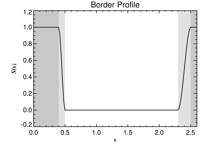
Figure 1: Border profile of the simulations. The step function (Eq. 13) is applied to the derivatives of the dynamical variables. The gas is free to evolve between $s$=0.5 and $s$=2.3, is slowed down between [0.4,0.5] and [2.3,2.5] (light-shaded areas) and is effectively frozen at $s<0.4$ and $s>2.5$ (dark-shaded areas).

To avoid numerical instabilities due to this abrupt jump from frozen to evolving regions, we apply a buffer zone to the derivatives of the variables, that smoothly drives the variable $X$ to a desired value $X_{0}$ in a timescale $\tau$, such that cp

$$\frac{\partial{X}}{\partial{t}}=-\frac{X-X_{0}}{\tau}\mathcal{S}(s).$$ (13)

where $\mathcal{S}(s)$ is the uniquely defined fifth-order step function that is 1 at the domain boundary and 0 at the interior boundary of the buffer zone while maintaining continuous second order derivatives (Dobler, private communication). Its shape is visualized in Fig. 1. We usually take the driving term $X_{0}$ to be the initial condition of the variable, and the driving time $\tau$ being the Keplerian period $2\pi/\Omega_{\rm K}$, the dynamical timescale of the disk. The effect of this border profile is to smooth the transition between the evolving disk and the frozen regions of the grid, thus preventing large gradients and discontinuities that would otherwise arise. As the gas flow is symmetric in the vertical direction, the vertical boundary condition is set to periodic for the purpose of simplicity.

For the runs without an inner boundary, we smooth the quantities containing singularities by replacing

$$s^{-n}\Rightarrow(s^{2}+b^{2})^{-n/2}.$$ (14)

In practice, it is applied to the angular frequency $\Omega$, the gravitational potential $\Phi$ and the sound speed $c_{s}$. We usually take $b=0.1$, so the smoothed gravitational potential deviates from the Newtonian by less than 5% at $s_{\rm int}=0.4$. The physical domain thus runs from $s_{\rm int}\,$to $s_{\rm ext}\,$.

For runs with an inner boundary, we apply inside $s_{\rm int}\,$the same freezing as used outside $s_{\rm ext}\,$. The $N$-body particle code does not participate in the freezing, so although the star lies in a region of frozen gas, it is allowed to move.

As the gas is frozen in the inner and outer parts, the information about the flow in this region is not of interest. Therefore, we exclude these regions from the time-step calculation. As their time derivatives are set to zero at the end of the time-step, they cannot violate causality.

In principle, we could set $s_{\rm int}\,$as close to zero as possible (by not using smoothing but retaining an inner boundary), in order to study the processes that happen in the immediate vicinity of the star, like winds, the magnetic cavity and surface accretion (von Rekowski & Piskunov 2006). However, due to the increasing Keplerian velocity in the advection and the decreasing resolution of the orbits, non-axisymmetric wave modes (particularly the $m$=4 mode) build up in the inner disk as we try to push $s_{\rm int}\,$$\rightarrow 0$. The density fluctuations resulting from the excitation of these modes lead to numerical instabilities.

Finally, the magnetic potential follows the same boundaries as described above. This would be a problem if we solved for the actual magnetic field, as sinks or sources of magnetic flux imply the presence of open magnetic loops (monopoles). By solving for the magnetic vector potential we do not face such problems.

The solid particles obey different boundary conditions, explained in Sect. 5.

3 Influence of free parameters

In order to clarify the influence of the numerical scheme and the approximations made, a series of non-magnetic 2D models were computed, with and without planets. The grid being Cartesian, all our simulations span the whole azimuthal domain. We usually evolve the simulations up to 100 orbits at $s_{0}$, which corresponds to $\approx$25 orbits at the outer edge of the disk and $\approx$400 orbits at its inner edge.

3.1 Viscosity

Explicit hyperviscosity and hyperdiffusion induce dissipation primarily near the grid scale, replacing the usual 2^nd order Laplacian terms. A visual picture of the difference between using the two types of viscosity is seen in Fig. 2. The first model was computed with a Laplacian viscosity $\nu_{1}=10^{-3}$. The radial inflow is significant, and as the outer frozen region behaves like an infinite reservoir of matter, the total mass inside the disk keeps on rising as matter flows in from this reservoir. The radial density profile soon starts to deviate from the flat initial condition . Shown in the figure is the density profile after 100 orbits at $s_{0}$ with $\nu_{1}=10^{-3}$. When using hyperviscosity of similar strength at the grid scale, i.e., $\nu_{3}=10^{-10}$, the overall flow shows no significant deviations from the initial conditions.

The simulation shown using Laplacian viscosity was computed without an inner boundary, using a softened stellar potential with $b$=0.1. Using the damping and freezing profile described in Sect. 2.7, the density is not allowed to deviate much from the initial condition at the boundaries. In the physically evolving part of the disk, however, a density profile of exponent $s^{-0.4}$ evolves.

3.2 Mass diffusion

To evaluate the influence of mass diffusion, we simulate a laminar disk with constant Laplacian viscosity $\nu_{1}=10^{-5}$ in the presence of a gap-opening Jupiter-mass planet. We performed runs of resolution $320\times 320$ with hyperdiffusion coefficients ranging from $D_{3}=5\times 10^{-11}$ to $10^{-14}$. After a hundred orbits, time enough for the planet to open a deep gap, the density profiles are plotted in Fig. 2a, where a run with resolution $640\times 640$ without explicit diffusion is shown for comparison.

It is seen that $D_{3}=5\times 10^{-11}$ constitutes too much diffusion, as the gap is significantly altered. As less diffusion is used, the shape of the gap monotonically approaches the one recovered in the higher resolution run. The walls of the gap are fairly well reproduced for lower diffusion, but its bottom is always shallower even for the lowest coefficient used ($D_{3}=10^{-14}$).

Judging from the gap alone, one could in principle use no diffusion at all, but the inner disk suffers depletion for low diffusion regimes, due to the non-conservative nature of the numerical scheme. Even the higher resolution run seems to have lost mass due to the lack of explicit diffusion.

We adopt a hyperdiffusion coefficient of $D_{3}=5\times 10^{-12}$ as the best compromise between the need for preserving material in the inner disk and for reproducing the overall shape of the gap. Requiring Schmidt and magnetic Prandtl numbers of 1 at the grid scale, we set hyperviscosity and hyperresistivity to the same value.

Figure 2: The radial density profile after 100 orbits for Laplacian viscosity $\nu_{1}=10^{-3}$ is compared to the profile obtained by using sixth-order hyperviscosity ($\nu_{3}=10^{-10}$) of same strength in the small scales. In the hyperviscous case, the global flow is unaffected. Note that the frozen regions behave like infinite reservoirs of matter. The power law describing the resulting density profile for normal viscosity is very close to the $s^{-0.5}$, as expected for constant viscosity (see Pringle 1981 and references therein)

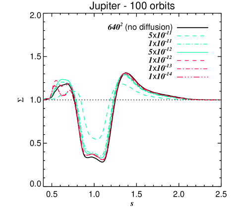
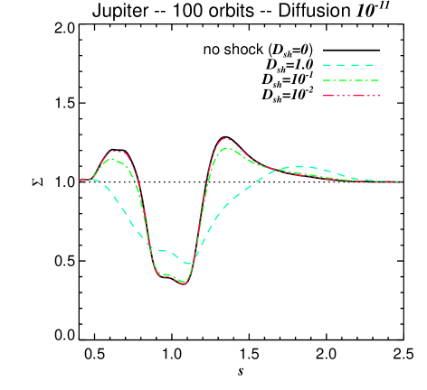
Figure 3: Upper Panel. The gap carved by a 1 $M_{J}$ planet in a 2D disk reveals the influence of explicit diffusion in the calculations. The inner disk loses mass depending on the amount of diffusion. The value of $D_{3}=5\times 10^{-12}$ seems to ensure mass conservation in the inner disk yet not distorting the shape of the gap. The solid line represents a $640\times 640$ run without diffusion, for comparison. Resolution is $320\times 320$ otherwise.
Lower Panel. Same but with hyperdiffusion set to $D_{3}=10^{-11}$ and varying the shock diffusion coefficient from $10^{-2}$ to $1$.

3.3 Shocks

Shock viscosity and shock diffusion are needed for two reasons: (a.) to stabilize the flow near the shock-generating particles in runs with planets and (b.) to treat eventual supersonic motion in the turbulence (arising when the disk is exposed to a strong net vertical field), in which case shock resistivity is also included.

In Fig. 2b we show gap-opening runs with fixed hyperdiffusion coefficient $D_{3}$ but varying the shock diffusion coefficient. From the continuity equation, one can tell that the effect of shock diffusion is to slow down the time evolution of density by smearing out any large divergences. Indeed, one sees that after a hundred orbits, a shock diffusion coefficient of $1$ fails to reproduce the shape of the gap as compared to the higher resolution run without shock diffusion, while $10^{-1}$ shows less accumulation than expected in the Lindblad resonances, also seen as compared to the higher resolution run. We therefore use shock diffusion of $10^{-2}$ for the turbulent runs. The flow around a high-mass planet, however, could only be stabilized with a shock viscosity of 1.

Shock resistivity is also used when the run involves the magnetic potential. The value used was not tuned in 2D runs like shock diffusion and shock viscosity. Instead, in the presence of turbulence, we simply checked what was the lowest shock resistivity coefficient that did not lead to numerical instabilities for model A (see Table 2), finding that it is of the order of unity, like the shock viscosity.

3.4 Non-turbulent runs

To verify the numerical stability of the model in the absence of physical turbulence, we perform tests for cases where the turbulence is not supposed to be present. In these runs, we monitor the evolution of the mass inflow rate $\dot{M}$ defined as the 1D radially dependent surface integral over a surface $\mathcal{A}$ which is a cylinder at a radial distance $s$ from the origin

$$\dot{M}(s) = \varoiint_{\mathcal{A}}\rho\,{\bm{u}}\cdot\hat{{\bm{n}}}\,\mathrm{d}{A}$$ (15)

$$= 2\pi s\int_{{}_{-L_{z}/2}}^{{}^{\,\,L_{z}/2}}\rho(s,z)u_{s}(s,z)\,\mathrm{d}{z}.$$ (16)

We see that in a 2D laminar model, the mass inflow rate is constant through the radial domain once a steady flow is achieved (which simply states that mass is conserved). We thus define the mass accretion rate as the mass inflow rate across the inner boundary,

$\dot{m}=\dot{M}|_{{}_{s=0.4}}$,

meaning that after crossing this boundary, the matter is considered lost (accreted).

We also measure the kinetic alpha parameter of turbulent viscosity, defined as

$$\alpha_{R}=\frac{2}{3}\frac{R^{s\phi}}{\rho c_{s}^{2}},$$

where $R^{s\phi}=\overline{\rho\delta u_{s}\delta u_{\phi}}$ is the Reynolds stress; and its magnetic counterpart

$$\alpha_{M}=-\frac{2}{3}\frac{M^{s\phi}}{\rho c_{s}^{2}},$$

where $M^{s\phi}=\mu_{0}^{-1}\overline{\delta B_{s}\delta B_{\phi}}$ is the Maxwell stress.

In Fig. 4 we show a 2D run where the velocities were perturbed with noise of $u_{\rm rms}=10^{-2}$, but the induction equation is not solved. The turbulence dies out so fast that even before ten orbits at $s_{0}$ the flow is already smooth, showing that the numerical scheme does not spuriously generate or sustain turbulence.

A 3D cylindrical run in which we add a vertical net field of strength $B_{0}=10^{-3}$ (dimensionless), corresponding to plasma $\beta$=5000 at $s_{0}$, 12500 at $s_{\rm int}\,$and 2000 at $s_{\rm ext}\,$(see Eq. [19]), but where the initial flow is not perturbed by noise, does not develop turbulence. We also tested if the MRI would develop in a disk seeded only with noise in both the velocity and magnetic potential ($u_{\rm rms}=A_{\rm rms}=10^{-4}$). There is a short growth in magnetic energy, presumably due to reconnection of the field lines, but without a structured field to maintain the turbulence the Reynolds and Maxwell stresses quickly level down to zero as viscosity and resistivity smooth the imposed noise.

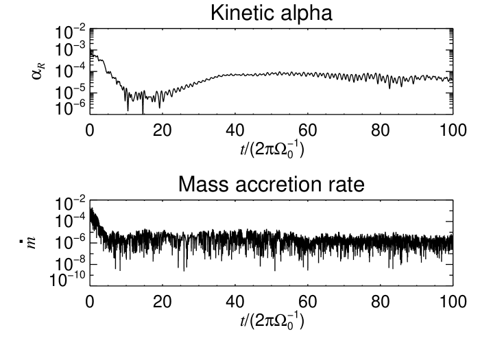
Figure 4: Without solving the dynamical equations for the magnetic field, even initially vigorous random motions of $u_{\rm rms}=0.2c_{s_{0}}$ die out rather quickly. The plots show the time evolution of the globally averaged Reynolds stress and mass accretion rate. Time is quoted in orbits at $s_{0}$.

Table 2: Cylindrical turbulent disk models.

Parameter

Results

Run

$s_{\rm int}\,$

$B_{0}$

$c_{s_{0}}$

$q_{{}_{T}}$

$\beta_{0}$

$N_{z}$

$\chi_{\rm sh}$

$N_{p}$

$R^{s\phi}$

$-M^{s\phi}$

$\alpha_{R}$

$\alpha_{M}$

$B_{\rm rms}$

$\beta_{t}$

$\delta_{t}$

($\times 10^{3}$)

($\times 10^{5}$)

($\times 10^{5}$)

($\times 10^{3}$)

($\times 10^{3}$)

($\times 10^{3}$)

($\times 10^{3}$)

Uniform Field $B_{z}$

A

0.4

1

0.05

1

5000

32

1

$10^{6}$

0.24$\pm$0.04

1.5$\pm$0.3

0.9$\pm$0.2

6$\pm$1

17$\pm$9

13$\pm$3

7$\pm$1

B

0.4

1

0.10

1

20000

32

1

…

1.0$\pm$0.2

2.5$\pm$0.3

0.7$\pm$0.1

1.8$\pm$0.2

16$\pm$5

65$\pm$7

…

C

0.4

1

0.20

1

80000

32

1

…

4$\pm$1

5.3$\pm$0.8

0.9$\pm$0.2

1.3$\pm$0.2

26$\pm$7

81$\pm$7

…

A 2

0.0

1

0.05

1

5000

32

1

…

0.20$\pm$0.04

1.3$\pm$0.1

0.7$\pm$0.1

4.7$\pm$0.3

17$\pm$5

13$\pm$1

…

B 2

0.0

1

0.10

1

20000

32

1

…

0.9$\pm$0.2

2.6$\pm$0.3

0.8$\pm$0.1

2.1$\pm$0.2

20$\pm$11

43$\pm$13

…

C 2

0.0

1

0.20

1

80000

32

1

…

5$\pm$3

5$\pm$1

1.2$\pm$0.8

1.2$\pm$0.3

22$\pm$9

116$\pm$19

-

Radially Varying Field $B_{z}$

D

0.4

20

0.10

2

12

64

2

$10^{6}$

22$\pm$2

78$\pm$7

25$\pm$1

87$\pm$3

71$\pm$9

4$\pm$1

140$\pm$10

E

0.4

20

0.20

2

50

64

2

…

35$\pm$7

87$\pm$15

13$\pm$3

30$\pm$5

60$\pm$23

11$\pm$1

…

Dw

0.4

5

0.10

2

750

64

2

…

4.1$\pm$0.4

13$\pm$2

5.4$\pm$0.6

17$\pm$2

28$\pm$10

13$\pm$2

…

Ew

0.4

5

0.20

2

3000

64

2

…

13$\pm$4

27$\pm$2

4$\pm$1

8.7$\pm$0.7

36$\pm$11

33$\pm$3

…

Uniform Field $B_{\phi}$

F

0.0

30

0.05

1

5.5

32

2

…

0.7$\pm$0.1

2.9$\pm$0.4

2.5$\pm$0.4

11$\pm$1

12$\pm$4

24$\pm$2

…

G

0.0

30

0.20

1

90

32

2

…

5$\pm$2

18$\pm$6

0.9$\pm$0.4

3.3$\pm$1.4

28$\pm$11

107$\pm$22

…

4 Cylindrical disk runs

For the main simulations in this paper we consider flat vertical profiles for the gravity field. Such an approximation is called a “cylindrical” disk and has been often used in order to study the MRI (e.g., Armitage 1998, Hawley 2001). The vertical gravity $g_{z}=-\Omega^{2}{\bm{z}}$ is switched off so that, physically, the star is no longer a point mass at $r$=0, but a rod at $s$=0 extending through the length of the $z$-axis. In such a setup, the pressure scale height $H$ has no hydrostatic meaning, being only a way to write the temperature profile of the disk. We performed simulations with non-zero net flux magnetic fields ${\bm{B}}=B_{0}\hat{{\bm{z}}}$ and ${\bm{B}}=B_{0}\hat{{\bm{\phi}}}$. Models with a radially varying vertical field proportional to $\Omega(s)$ were also computed.

For the turbulence to develop, the unstable wavelengths of the MRI must be resolved. The characteristic vertical wavelength $\lambda_{\rm BH}$ of the hydromagnetic turbulence is given by (Balbus & Hawley 1991, 1998)

$$\lambda_{\rm BH}=2\pi\frac{v_{{}_{\rm A}}}{\Omega},$$ (17)

where $v_{{}_{\rm A}}$ is the Alfvén speed

$$v_{{}_{\rm A}}=\frac{B}{\sqrt{\mu_{0}\rho}}.$$ (18)

The turbulence will be present as long as the critical wavelength $\lambda_{c}$ is resolved. This wavelength is $\lambda_{c}=\lambda_{\rm BH}/\sqrt{3}$, whilst the most unstable wavelength of the MRI is $4\lambda_{\rm BH}/\sqrt{15}$ (Balbus & Hawley, 1991). The plasma $\beta$ parameter - the ratio of thermal to magnetic pressure - can be expressed in terms of the sound and Alfvén speed, by writing the magnetic pressure $P_{M}=B^{2}/(2\mu_{0})$ in terms of the Alfvén speed $P_{M}=B^{2}/(2\mu_{0})=\rho v_{{}_{\rm A}}^{2}/2$, giving

$$\beta=\frac{2c_{s}^{2}}{v_{{}_{\rm A}}^{2}}.$$ (19)

The constant $B_{0}$ is usually set to $10^{-3}$, but runs varying the field from $10^{-4}$ to $10^{-1}$ were also studied. Although the runs reported here are in the local isothermal approximation, we also varied the initial sound speed at $s_{0}$, $c_{s_{0}}$, in order to check how the resulting turbulent viscosity depends on the global gas pressure.

The parameters of the cylindrical models presented here are specified in Table 2.

4.1 Constant vertical field - model A

The evolution of the turbulence in a fiducial run with a net vertical flux of strength $B_{0}=10^{-3}$ and temperature profile corresponding to $c_{s_{0}}=0.05$ is shown in Fig. 5. The absolute value of the Maxwell stress at saturation is always larger than the Reynolds stress, but the latter fluctuates more strongly.

The minimum ratio of stresses is $-M^{s\phi}/R^{s\phi}$=3 (at t$\approx$75 orbits), but it reaches as much as 100 (at t$\approx$58 orbits). After 75 orbits, the average ratio of Maxwell to Reynolds stress is around 5.

In agreement with previous shearing box simulations (Brandenburg et al. 1995, Hawley et al. 1995, Johansen & Klahr 2005), global disks (Hawley 2001, Nelson 2005) and analytical calculations (Balbus & Hawley 1991), a large scale toroidal field is seen to form, which dominates the magnetic energy, being 2 orders of magnitude stronger than the radial and vertical fields. Indeed, one can barely distinguish between the energy stored in the azimuthal field and the total magnetic energy. The kinetic energy is more evenly distributed, but it is not isotropic. The radial component accounts for 45% of the total energy, being $\approx$1.5 bigger than the vertical and twice as big as the azimuthal. The radial structure of the alpha parameter is seen in Fig. 6. The outer disk is more turbulent due to the smaller values of plasma $\beta$ when compared to the inner disk.

Following the time evolution of the turbulence in the midplane, it is seen that different regions of the disk reach saturation at different times. The turbulence starts from the outer disk, propagating inwards. It is expected since, as $\Omega$ decreases with radius, a uniform field implies a Balbus-Hawley wavelength that increases with distance from the star. As longer wavelengths - comparable to the length of the box - are easily resolved, the outer disk goes turbulent first. It is seen that inside $s_{0}$=$1$ the disk did not go turbulent. In this model, the Mach number is constant, ${\mathcal{M}}$=$20$, with a constant field, $B$=$10^{-3}$ through the whole domain, corresponding to plasma $\beta$ running from 2000 at $s_{\rm ext}\,$and 12500 at $s_{\rm int}\,$. The magnetic field determines the value of the critical wavelength, which ranges from $\lambda_{c}$=0.002 at $s_{\rm int}\,$to $\lambda_{c}$=0.025 at $s_{\rm ext}\,$. As we have 32 grid points in the vertical direction, the smallest wavelength resolved with significant accuracy (8 points) by our high-order finite-difference method is $L_{z}$/4$\approx$0.12. From the dispersion relation of the MRI (Hawley & Balbus 1991), this unstable wavelength has a growth rate of $\approx 0.1\Omega$, much lower than the fastest growing wavelength with $\omega=(3/4)\Omega$.

We also computed models where the whole disk goes turbulent (models D & E), but we will use these weak field disk models (models A to C2, see Table 2) in the next subsection for studying the behavior of the turbulence with thermal pressure. Although dissipative and slowly growing, the weak field used in these disks has one major advantage: the turbulence grows slowly and has less spatial variability. Therefore, the damping at the frozen boundaries is more gentle than in other, rapidly growing, violently fluctuating, disks. These issues discussed above reflect the compromise between keeping the disk cold while still retaining the field subthermal and with sufficient resolution to resolve the rapidly growing unstable wavelengths.

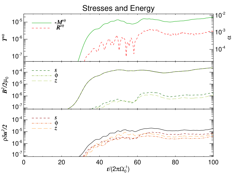
Figure 5: Time evolution of the turbulence for model A (constant net flux vertical field ${\bm{B}}=10^{-3}\hat{{\bm{z}}}$ and constant Mach number). The top panel shows the evolution of the $s\phi$-component of the Maxwell and Reynolds stresses, while the middle and bottom panels show the evolution of magnetic and kinetic energy, respectively. The units are given in Table 1. The solid lines in the two bottom panels show the total energy. The toroidal field dominates the magnetic energy to the point that the energy in the azimuthal component can barely be distinguished from the total energy. The kinetic energy is more evenly distributed among the three dimensions, but the turbulence is not isotropic. The radial component shows 1.5 times more energy than the vertical and 2 times more than the azimuthal. Time is quoted in orbits at $s_{0}$.

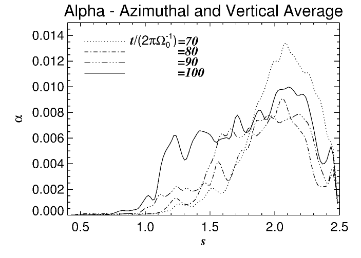
Figure 6: Radial structure of the total alpha parameter $\alpha_{R}+\alpha_{M}$ for model A . The turbulence starts from the outer disk, where plasma $\beta$ is smaller. The different curves correspond to snapshots at 70 (dotted), 80 (dot-dashed), 90 (dot-dot-dot-dashed), and 100 orbits (solid), after saturation is reached. The variability is not monotonic, but highly fluctuating.

The runs with a vertical net field of $B_{0}=10^{-4}$ or lower did not develop turbulence as the field is weaker than needed in the presence of the chosen dissipation parameters (Hawley & Balbus 1991).

4.2 Dependence on sound speed - models B and C

We investigate the dependence of the saturated state on the imposed sound speed profile. We test three different sound speeds of, $c_{s_{0}}$=0.05, 0.10 and 0.20, corresponding to runs A, B and C.

As the runs are locally isothermal, we are mainly investigating how the MRI responds to different radial pressure gradients. The cold model (A) shows a weaker turbulence at saturation than the hotter ones, as shown by the strength of the stresses (Fig. 7a,b) and magnetic/kinetic energies (Fig. 7c,d). The Maxwell stress is three times bigger for model C than for A, the colder version. Such behavior was reported by Sano et al. (2004), indicating a power law of exponent 0.25 for the growth of the Maxwell stress with gas pressure. Our global disk calculations agree well with this value.

The dimensionless magnetic $\alpha_{M}$ parameter, which is a measure of turbulent viscosity, decreases drastically with sound speed (Fig. 8). As seen before, the stresses actually increase with increasing temperature, so this decrease of $\alpha_{M}$ is due to the stresses increasing less rapidly than the temperature. Even though alpha decreases, the effective viscosity $\nu_{\rm t}$=$\alpha c_{s}H$ increases. As seen in Fig. 9 and Fig. 10, a centrally concentrated density profile has developed from the initially flat configuration, a signature of mass accretion due to turbulent angular momentum transport, as also confirmed by the measured stresses. The resulting density profile in model C is smoother overall, but the overdensities seem to be similar in average.

It is clear that alpha per se is not a good measure of viscosity. Since $\nu_{\rm t}=\alpha c_{s}^{2}\Omega^{-1}$, with no reference to the Alfvén speed, the resulting alpha value of turbulent disks where the origin of the turbulence is magnetic may change with sound speed. As most of the analyses of turbulent thin accretion disks have focused on locally isothermal simulations using $c_{s}\approx 0.05$, such dependence of $\alpha$ on sound speed did not receive proper attention. Although protoplanetary disks are thin, this rise in angular momentum transport with temperature suggests that the effects of radiation will be important for high temperature regions around forming planets as well as regions where the turbulence leads to significant Joule and/or viscous heating.

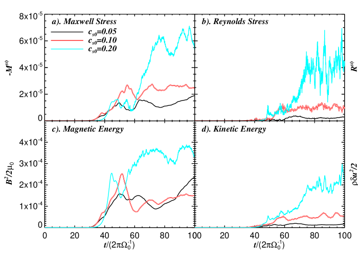
Figure 7: Time evolution of the turbulence for different sound speed profiles. The strength of the angular momentum transport differs with sound speed. The increase in stress observed when the sound speed is raised to $c_{s_{0}}=$0.20 is dramatic. Time is quoted in orbits at $s_{0}$.

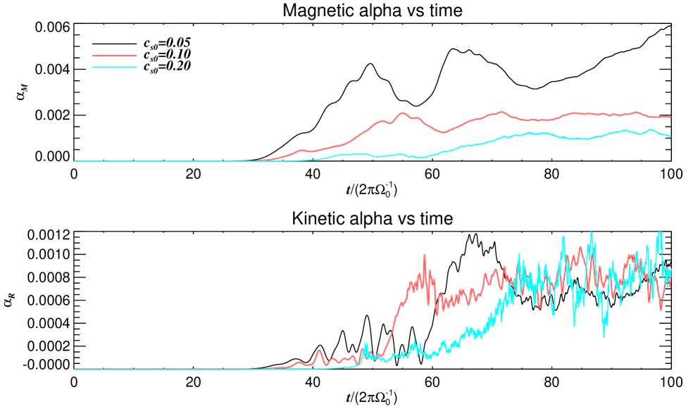
Figure 8: Evolution of the alpha parameters for different sound speed profiles. This quantity, that measures the strength of viscosity through the parametrization $\nu_{\rm t}=\alpha c_{\rm s}H$, decreases with sound speed for the magnetic stresses but stays constant for hydrodynamic stresses. As seen before, the stresses actually increase with increasing temperature, so this decrease of the alpha parameter is due to the stresses increasing less rapidly than the pressure. Time is quoted in orbits at $s_{0}$.

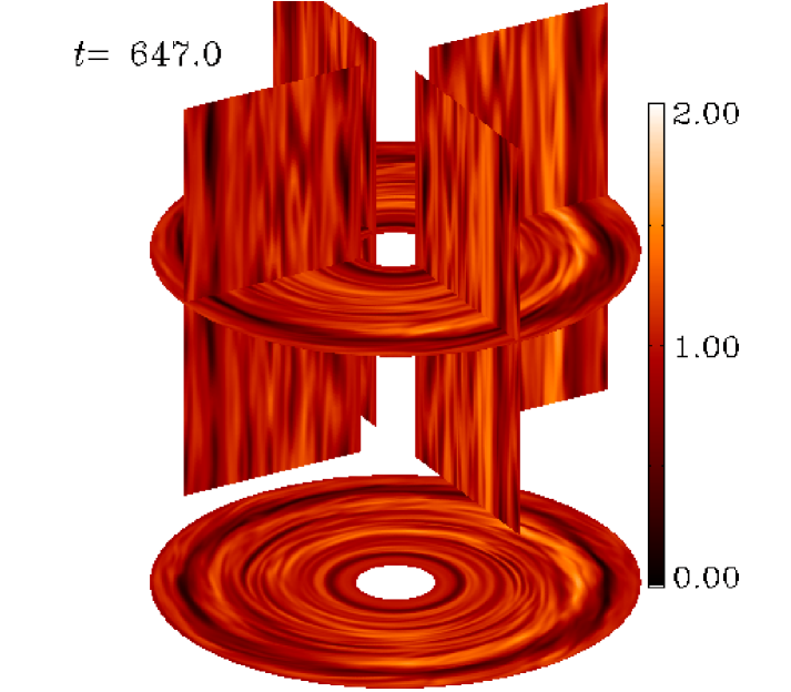
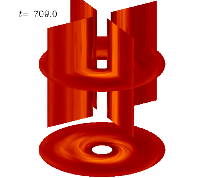
Figure 9: Density contours at selected planes $x$=$0$, $y$=$0$, and $z$=$0$ on saturated turbulent state for sound speed profiles of $c_{s_{0}}=0.05$ (model A, left panel) and $c_{s_{0}}=0.20$ (model C, right panel). The color code is the same for both figures. The stronger stresses for the hotter case lead to a much more effective turbulent viscosity, as seen from the steep density profile resulting from accretion. The vertical planes are stretched to show more detail than the correct aspect ratio would allow. Movies of these simulations can be found at http://www.astro.uu.se/$\sim$wlyra/planet.html.

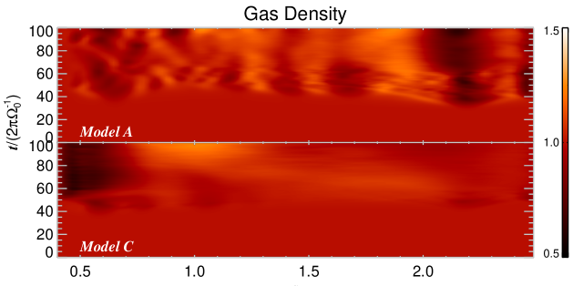
Figure 10: Radial density profiles for models A and C. The lower panels show space-time plots of the vertically and azimuthally averaged density. Model A shows what seems to be a variability around a constant value, model C has developed a smoother radial density gradient. The lower panel shows the two density profiles at the end of the simulation.

4.3 Excluding the inner boundary

The correct treatment of boundaries is a major issue for numerical simulations. In global simulations of disks, outflow or frozen boundaries are usually used, both of them being more realistic than reflective, but also presenting disadvantages. Strictly speaking, a “perfect” boundary might well not exist. The best solution would be, of course, not having to use a boundary at all.

Cylindrical grids only make sense if the center of mass is at the origin of the coordinate system as only then angular momentum transport can be written in a conservative form. If the center of mass is not at the origin or there is more than one massive object the cylindrical coordinate system artificially introduces a reflective boundary at the center. Cartesian grids, as stated before, are not hindered by this, and we can therefore study how the presence or absence of an inner boundary affects the results.

We compute a version of model A where the computational domain extends all the way to $s_{\rm int}\,$=0. Without an inner boundary, the gravitational potential, the angular frequency and the sound speed have to be smoothed according to Eq. (14) to prevent singularities. When taking global averages, we exclude the smoothed region.

The evolution of the turbulence and the globally averaged stresses at saturation are almost identical to those seen at model A. The only noticeable difference is that the highly fluctuating magnetic field observed in the inner boundary of model A (with rms amplitude $\approx$ 2 times seen in the rest of the disk) does not occur in this model.

In model A, the magnetic potential at the inner boundary remains frozen at the initial condition ${\bm{A}}$=$0$. As the MRI builds up the magnetic potential in the freely evolving disk, a sharp radial gradient appears at the boundaries. This sharp radial gradient in the azimuthal and vertical components of the magnetic potential translates into high values of the magnetic field. If we were solving for the magnetic field instead, a similar effect would be seen. The magnetic field would rise in the disk, but is kept frozen at the boundary, thus building up a high magnetic pressure with equally damaging effects for the simulation.

By avoiding the inner boundary altogether, such an effect does not occur. However, other problems arise as the advection on the very inner disk ($s$$<$0.4) happens on tight circular trajectories that are poorly resolved in the Cartesian geometry near the center of the grid. As they behave like highly localized vortices, in most cases the explicit shock dissipation terms ensure numerical stability. But for cases with stronger turbulence (model D, Sec 4.4), a model without an inner boundary could not be treated.

As we did for the models with an inner boundary, we check the dependency of the turbulent stresses with sound speed by computing versions of models B and C without an inner boundary. As for model A2, these models B2 and C2 behave quite similarly to models B and C, saturating at roughly the same stresses.

4.4 Radially varying field - models D and E

With the constant vertical field, it is seen that the inner disk does not go turbulent. This is due to the fact that in this rapidly advecting region, the growth of the MRI is numerically damped.

In view of this, we also compute models with a radially varying $z$-field

$${\bm{B}}=\frac{L_{z}\Omega(s)}{2j\pi}\sqrt{\mu_{0}\rho_{0}}\hat{{\bm{z}}},$$ (20)

such that $j$ Balbus-Hawley wavelengths (Eq. [17]) are resolved through the vertical extent $L_{z}$ of the box at any radius. We computed a model with $j=4$ (model D), and another version, with a weaker field (model Dw) with $j=16$, so that unstable wavelengths are reasonably well resolved. These fields can make the whole disk go turbulent, but they grow so strong in the inner disk of model D that a more pronounced temperature profile ($q_{{}_{T}}$=$2$) had to be used to avoid the magnetic field from going superthermal. For model D, such a setup has plasma $\beta$=20 at $s_{\rm int}\,$and 120 at $s_{\rm ext}\,$. Model Dw has a field with a strength more similar to model A, and therefore would not need this fix. However, to allow a comparison with model D, we also used this steeper temperature gradient, thus having a plasma $\beta$= 300 at $s_{\rm int}\,$and 1850 at $s_{\rm ext}\,$.

As this setup has an inverse $\beta$ profile compared to the models with a constant vertical field, the turbulence starts from the inner disk instead of the outer. Also, as the magnetic field is stronger, wavelengths of faster growth rate are better resolved and the turbulence saturates after a few orbits. Due to the strong stresses, we had to raise shock resistivity to 2 instead of 1 as used before.

The stresses also saturate at higher values, 0.08 for the Maxwell stress, and 0.02 for the Reynolds stress (Fig. 11) for model D. The weaker field yields a total alpha viscosity around $2\times 10^{-2}$ ($\alpha_{M}$=0.017 , $\alpha_{R}$=0.005, see Fig. 11a and Table 2). These values are at least one order of magnitude higher than the ones obtained with a constant field. The radial structure of the alpha value, plotted in Fig. 12, reveals that the stresses follow the radial profile of 1/$\beta$, being stronger in the inner disk. The same was seen in the simulations with a constant field, where the stresses were stronger in the more magnetic outer disk.

The stresses in this model are so high that the alpha viscosity in the saturated state is always of the order $10^{-1}$, reaching $\approx$0.5 in the more magnetized inner disk (Fig. 12). That means that the inner disk approaches magnetically dominated values for plasma $\beta$ as the turbulence saturates. The global average of plasma $\beta$ in the saturated state is 4, although it did not reach superthermal values ($<$1) during the course of the simulation. Model Dw is milder, having a total alpha value of the order $10^{-2}$, reaching a maximum of $\approx$0.08 in the more magnetized inner disk.

The high stresses compared to the cases with constant vertical field stem from the initially stronger magnetic field, not from a pressure effect. Indeed, in this setup, the temperature profile is steeper, but it never rises above the sound speed of model C, with $c_{s_{0}}=0.2$ and power law of exponent $0.5$. However, we still expect the pressure effect seen on models ABC to be present. To check the behavior of this setup with the imposed temperature profile, we compute another model (model E) with the same initial condition for the magnetic field as model D, but with a hotter temperature, with $c_{s_{0}}=0.2$. This setup has a plasma beta value of 80 in the inner disk and 450 in the outer. A weaker version with plasma beta value of 1200 in the inner disk and 7400 (model Ew) was also computed, for comparison with model Dw. The results (Fig 11b) are similar to models ABC: The stresses are indeed larger than those of model D and Dw, but the alpha viscosity values are smaller. Also as seen on models ABC, the kinetic alpha did not change appreciably, but the magnetic alpha was reduced by approximately a factor of 2.

The ratio of stresses varied as well, as seen in models ABC. It is around 4 for model D, but 2 or less for model E. It is around 3 for model Dw, but less than 2 for model Ew.

A final note on the temperature effect; we see that, like alpha, the turbulent plasma beta parameter $\beta_{t}$ does not scale with pressure. As the rise in the turbulent magnetic energy is outpaced by the growth of the pressure, $\beta_{t}$ increases with increasing temperature.

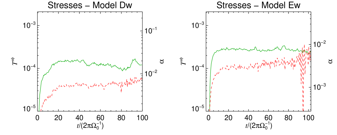
Figure 11: Time evolution of the turbulent stresses for models D and E (upper panels) and Dw and Ew (lower panels). As compared with model A, the stresses saturate at a much earlier time. The ratio of Maxwell to Reynolds stress is around three for model D, and around two for the hotter model E, approaching one at the end of the simulation. Notice that as seen in models ABC, the stresses are bigger for the hotter model, although the alpha viscosity value is smaller. Time is quoted in orbits at $s_{0}$.

Figure 12: Same as Fig. 6, but for models D (left panel) and Dw (right panel). The times corresponding to the snapshots are indicated in the legends, as well as the time average. The inner disk is considerably more turbulent than the outer parts.

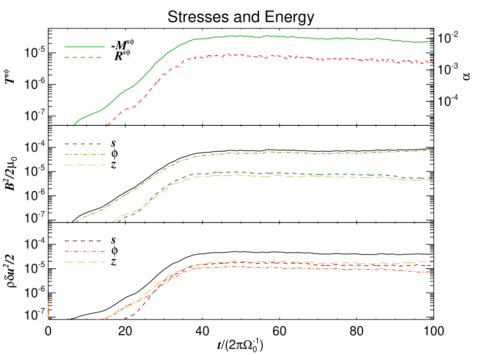
Figure 13: Same as Fig. 5 (constant vertical field), but for model F (constant azimuthal field).

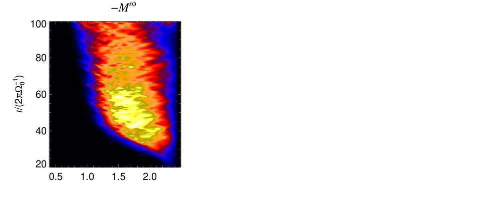
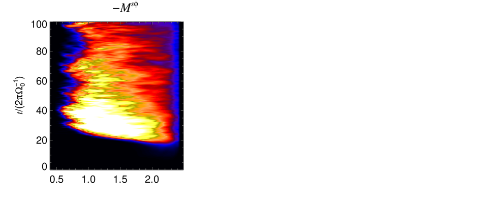
Figure 14: Space-time diagram of the turbulent stresses and alpha viscosity for model F (upper panels) and model G (lower panels). Time is quoted in orbits at $s_{0}$=1.0. Saturation is reached at 40 orbits, but after 60 orbits the stresses seem to start a slow decay. The alpha viscosity appears constant, due to a similar decay in gas pressure in the outer disk, that starts to deplete as the resulting accretion builds a negative density gradient. Model G behaves similarly, but with higher stresses, lower alpha viscosity and being turbulent further inside.

4.5 Constant azimuthal field - models F and G

Analytical treatment (Balbus & Hawley 1992, Ogilvie & Pringle 1996) and numerical simulations (Hawley 2000, Papaloizou & Nelson 2003) show a wealth of evidence that the MRI also exists for a purely toroidal field. In this case, waves of the form $\exp[i(m\phi-\omega t)]$, where $m$=$k_{\phi}s$ is the azimuthal wavenumber, are excited. The maximum growth rates are similar to those observed in purely vertical fields, but reached at much smaller azimuthal wavenumbers.

For an azimuthal field, the maximum growth rate occurs at the wavenumber (Balbus & Hawley 1998)

$$m_{\small{\rm max}}(s)=\frac{\sqrt{15}}{2}\frac{\Omega s}{v_{{}_{\rm A}}}$$ (21)

Such wavelengths are now resolved in the $xy$ plane, instead of in the vertical direction. Without the severe constraint of fitting unstable wavelengths in the tiny vertical scale height of the disk, the azimuthal field can be set at much stronger values than those used in the vertical cases. The only constraint is that we keep the field subthermal. With a temperature gradient of $q_{{}_{T}}$=$1$ and $c_{s_{0}}$=0.05, a constant azimuthal field of $B_{0}$=$3\times 10^{-2}$ (model F) corresponds to plasma $\beta$ of 12 at $s$=0.4, 5.5 at $s_{0}$ and 2 at $s$=2.5. The wavenumbers are $m_{\small{\rm max}}$=65 at $s_{0}$, 102 at $s$=0.4 and 41 at the outer boundary. A hotter version, with $c_{s_{0}}$=0.20, yielding plasma $\beta$=220 at $s$=0.4, 90 at $s_{0}$ and 35 at $s$=2.5 (model G), was also computed for comparison.

Following the time evolution of model F, we see that the turbulence actually saturates at $t$=200 at $s$=2.0 ($\approx$ 11 orbits), $t$=300 at $s$=1.5 ($\approx$ 30 orbits) and is still growing linearly at $s$=1.0 at the end of the simulation at $t$=628 (100 orbits). The global average (fig. 13), and a space-time $(s,t)$ inspection (fig. 14) of the stresses reveals that after reaching saturation at $t$=250 (40 orbits at $s_{0}$), a steady state is maintained for 20 orbits, after which the turbulence starts decaying slowly. But as a small growth is observed near the end of the simulation, it is not clear if this decay would continue to zero or if it constitutes just a unusually long fluctuation of the turbulence. Moreover, the magnetic and kinetic energies (fig. 13) show no signs of decaying.

On the right panel of fig. 14, we plot the total alpha viscosity parameter $\alpha_{M}+\alpha_{R}$. Curiously, it does not show the decaying effect seen on the stresses, implying that a decrease in gas pressure accompanied the decrease in Maxwell stress. Such a behavior is expected, since a negative density gradient is arising from the accretion process. Therefore, a depleted outer disk has a larger value of alpha viscosity for the same Maxwell stress.

The global average yields $R^{s\phi}$=(0.7$\pm$0.1)$\times 10^{-5}$, $M^{s\phi}$=(2.9$\pm$0.4)$\times 10^{-5}$ and total alpha viscosity $\alpha$=(1.3$\pm$0.1)$\times 10^{-2}$.

Model G shows Maxwell stresses that go further towards the inner disk, and Reynolds stresses that extend to inside $s$=$0.4$ as seen in Fig. 14. The outer disk attains a turbulent state first, at $t$=100 (15 orbits), and the inner disk at $t$=200 (30 orbits). The turbulent alpha parameter peaks at $8\times 10^{-3}$ ($\alpha_{M}$=$6\times 10^{-3}$, $\alpha_{R}$=$2\times 10^{-3}$) at 30 orbits and starts a long decay until leveling after other 30 orbits at $\alpha_{M}$=$3\times 10^{-3}$ and $\alpha_{R}$=$7.5\times 10^{-4}$. The global averages are $R^{s\phi}$=(5$\pm$2)$\times 10^{-5}$, $M^{s\phi}$=(1.8$\pm$0.6)$\times 10^{-4}$ and total alpha viscosity $\alpha$=(4.2$\pm$1.5)$\times 10^{-3}$.

The referee, Dr. Ulf Torkelsson, pointed out to us that the non-zero tension of the constant azimuthal field,

$$\mu^{-1}({\bm{B}}\cdot{\bm{\nabla}}){\bm{B}}=-\mu^{-1}B_{0}^{2}s^{-1}\,\hat{{\bm{s}}}\,,$$

leads to an increase in the centripetal force that is not taken into account by Eq. (12), so the models with azimuthal flux are not started in strict magnetohydrostatical equilibrium. We therefore performed a set of 2D tests to assess how this out-of-equilibrium initial condition could modify our results. First we ran a 2D disk without noise in the velocity field, so although a magnetic field is present, the spectrum of wavelengths is not excited. The departure from equilibrium launches a sound wave starting from the inner disk and propagating outwards. At time $t$=30 ($\approx$5 orbits) in model F the sound wave reaches the outer boundary and is damped by the buffer zone. After that, the oscillations slowly damp through the next orbits as the disk settles into centrifugal equilibrium between gravity, thermal pressure, and magnetic tension forces. We followed the evolution until time $t$=90. At this time, the amplitude of the perturbation dropped to 3% of the initial density and 1% of the reference sound speed $c_{s0}$.

In model G, with a sound speed 4 times faster, the sound wave reaches the outer boundary much earlier, at time $t$=12 (about 2 orbits). By including noise we see the same results, so we conclude that in a 2D case, even though the non-vanishing magnetic tension leads to an out of equilibrium initial configuration, the discrepancy is slight and the system quickly relaxes in a timescale that is much smaller than the time the MRI takes to saturate (20 orbits).

5 Disks with solid boulders

Having presented the gaseous disk models, we now proceed to study the behavior of solid boulders inserted in these disks we have constructed. Meter-sized boulders are an important step towards kilometer-sized planetesimals. They are also interesting from a gas-dynamical point of view because they are only marginally coupled to the gas (on approximately a Keplerian shear time-scale) and can thus experience concentrations in vortices and transient gas high pressures (Barge & Sommeria 1995, Fromang & Nelson 2005, Johansen et al. 2006)

Our models are usually evolved for $\approx$75 orbits at $s_{0}$ before we add the particles, to allow for the turbulence to develop and saturate. A large number of particles ($10^{6}$) is used, which allows us to trace the swarm of particles onto the grid as a density field. The initial condition is such that the particles are concentrated in an annulus of constant bulk density $\rho_{p}$, ranging from $s_{\rm int}\,$to $s_{\rm ext}\,$, with a solids-to-gas ratio of 0.01, typical of the interstellar medium. Their velocity is initially the Keplerian angular velocity for their radial location.

As boundary conditions, we do not allow the particles to leave the computational domain as they drift inwards due to gas drag from the slightly sub-Keplerian gas. Instead, a particle that crosses the inner radius $s_{\rm int}\,$will be relocated to the outer radius $s_{\rm ext}\,$, where it will reappear at the same azimuthal location, thus mimicking periodic boundary conditions. Its velocity, however, will be reset to the Keplerian angular velocity at $s_{\rm ext}\,$. A particle that tries to cross the outer radius will simply have its velocity reset to Keplerian without changing its radial or azimuthal location.

We include particles at the later stages of models A and D. For model A, where the inner disk does not go turbulent, it was noticed that by allowing the particles to move through all the radial range, they eventually got trapped in the several local density maxima between the concentric rings that the inner disk breaks into. As such a loss of particles is undesirable, we keep them where the turbulence is saturated by setting the inner radius of the boundary conditions for particles outwards of $s_{0}$. In model D, where the Balbus-Hawley wavelength is resolved at all radii, such correction is not needed. We discuss the results of model D first.

5.1 Particles on model D

The particles soon fall to the disk midplane due to the vertical gravity. At the same time they get trapped in high pressure regions in the turbulent flow due to the drag force (Klahr & Lin 2001, Johansen et al. 2006). In Fig. 15 we plot a slice of the bulk density of solids profile 10 orbits after the insertion of the particles into the simulation. A pile-up of solids in the inner disk is seen to have occurred, because particles have concentrated in a pressure maximum in the gas (we discuss this further in Sect. 5.2; see also Fig. 18).

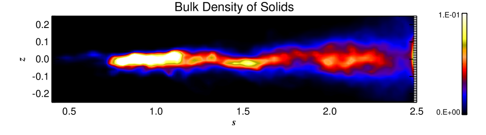
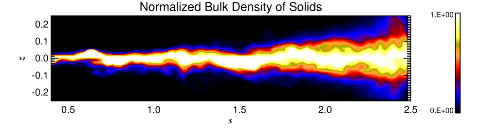
Figure 15: Vertical slice of the bulk density of solid particles (upper) and the same quantity normalized by the midplane density. A midplane layer forms in equilibrium between sedimentation and turbulent diffusion. The scale height of this layer follows a linear dependence with radius.

As discussed by Johansen & Klahr (2005), while solid particles are pulled towards the midplane by the stellar gravity, turbulent motions stir them up again. A sedimentary layer in equilibrium between turbulent diffusion and gravitational settling is formed. The thickness of this layer is therefore a measurement of the turbulent diffusion acting on the solid particles.

Under the influence of gravity, the solids settle with a profile similar to the one generated by a pressure force (Dubrulle et al. 1995)

$$\ln\rho_{\rm p}(s,z)=\ln\rho_{\rm p}(s,z=0)-\frac{z^{2}}{2H_{\rm p}^{2}}.$$ (22)

By comparing this profile with the analytical expression for a pressureless fluid under diffusion, gas drag and vertical gravity (Johansen & Klahr, 2005)

$$\ln\rho_{\rm p}=\ln\rho_{\rm p}(s,z=0)-\frac{\tau_{f}}{D_{z}^{(t)}}\int g_{z}\,{\mathrm{d}}z,$$ (23)

and recalling that $g_{z}=-\Omega^{2}z$, we have

$$D_{z}^{(t)}=\Omega^{2}H_{\rm p}^{2}\tau_{f}$$ (24)

From Eq. (22), we see that the scale height of the solids is the vertical distance in which the bulk density falls by a factor $1/\sqrt{\mathrm{e}}\approx 0.6$ relative to the value at midplane. We plot in Fig. 15b the bulk density normalized by its value in the midplane. In this figure, the quantity plotted is in fact identical to the exponential term in Eq. (22). Where it reaches 0.6, the vertical distance $z$ gives the diffusion scale height $H_{\rm p}$.

We fit the points where the exponential term equals 0.6 with a power law $H_{\rm p}=ar^{n}$. A linear regression in logarithm yields $a=0.042$ and $n=0.97$, with an rms of 0.04. This translates into a diffusion coefficient (Eq. [24]) of $D^{(t)}\approx 1.7\times 10^{-3}\,s^{-1}$. As this model has a sound speed profile $c_{s}$=$0.1\,s^{-1}$, the diffusion coefficient in dimensionless units corresponds to $\delta^{(t)}=D^{(t)}c_{s}^{-2}\Omega=0.17\,s^{-1.5}$, or 0.14 if globally averaged. The rms of 0.04 in the logarithm fit yields an uncertainty of 0.01 in this global average. As the total alpha viscosity is 0.112$\pm$0.003, the globally averaged vertical Schmidt number, i.e., the strength of viscosity when compared to vertical diffusion, is 0.78$\pm$0.06.

5.2 Particles in model A

For model A, the alpha viscosity ($\alpha\sim 10^{-3}$) is much lower than in model D ($\alpha\sim 10^{-1}$), so according to Eq. (24) and assuming that the diffusion coefficient is of the same order of the turbulent viscosity, we expect the sedimentary layer of solid particles to have a scale height of $H_{\rm p}=\alpha/\Omega^{2}\tau_{f}\approx 0.03H$. At $s_{\rm ext}\,$, the gas scale height $H$ equals 0.08 for $c_{s_{0}}=0.05$, then $H_{\rm p}=2.5\times 10^{-3}$. With a grid resolution $\Delta z=0.02$, this layer will not be resolved. It means that the interpolation of the particle density back to the grid will not allow for a grid-based measurement of the diffusion acting in the turbulent layer as we did for model D.

But as the particles are Lagrangian, we can plot their real positions and trace the scale height of solids in a grid-independent way. The diffusion process operates in much the same way, nearly independent of grid resolution, since the large scale velocities of the gas are well resolved. In order to do this, we define 128 bins in the radial direction and measure the individual vertical positions of the swarm of particles with respect to the midplane of the disk within these bins. The standard deviation $z_{\rm rms}$ of the vertical positions of particles with respect to the midplane in each bin immediately gives the scale height of the sedimentary layer. The result of this process is shown in Fig. 16a, where we average $z_{\rm rms}$ as measured on 17 snapshots, from orbits 4 to 20 at $s_{0}$ after the insertion of the particles. The initial time is chosen at 4 orbits because it is the time it takes for the drag force to couple the particles to the gas at $s_{\rm ext}\,$, thus making sure that the sedimentary layer is in equilibrium between gravitational settling and turbulent diffusion through the whole radial extent of the disk.

The dashed line in Fig. 16a represents the power law fit $H_{\rm p}$=$ar^{n}$ to the measured scale height. It yields $a$=$0.003$ and $n$=$2.48$. The rms of the logarithmic fit is $0.09$. In Fig. 16b we plot the resulting diffusion coefficient $D_{z}^{(t)}$=$\Omega^{2}H_{\rm p}^{2}\tau_{f}$. It can be approximated by a power law of $\approx 9\times 10^{-6}\,s^{2}$. In dimensionless units it corresponds to $\delta^{(t)}$=$3.6\times 10^{-3}\,s^{-1.5}$, or 0.007 if globally averaged. The uncertainty is 0.001. This behavior of the turbulent diffusion that acts on solids is quite similar to the one shown by the turbulent viscosity arising from the stresses on the gas phase (dot-dashed line in Fig. 16b). Checking the radial dependency of the Schmidt number (Fig. 16c), we see that it is of the order of unity all over the radial domain. A slight trend is seen towards smaller Schmidt numbers in the outer disk, but it never gets below 0.6.

In Fig. 17 we explore this radial dependency in more detail. The figure shows the vertical and azimuthal average of the turbulent viscosity $\nu_{t}$, turbulent diffusion $D_{t}$ and their ratio Sc, the Schmidt number, as a function of radial position $s$. On the time axis we show time in orbits at $s_{0}$ since the beginning of the simulations. At 71 orbits the particles are inserted, and quickly fall to the midplane. As seen from the diffusion map, the particles in the innermost radii quickly sediment, settling in a diffusive equilibrium in less than two orbits. After four orbits, $t=75$, the last radius achieves diffusion equilibrium and the situation becomes statistically unchanged until the end of the simulation.

The gas-phase viscosity and the solid-phase diffusion are similar in average, but the diffusion is seen to fluctuate more. Transient patches of high diffusivity are seen to live for some orbits at a constant radial location before decaying. The turbulent viscosity, in turn, appears much smoother in time. The resulting Schmidt number is shown in greyscale in the right panel of Fig. 17. Due to the high variability of diffusion, some short lived bright areas of Sc$>$5 are seen, but overall the Schmidt number is around 1 throughout the space-time domain.

In Fig. 18 we show contours of the gas density (left panel) and the bulk density of solids (right panel) in a snapshot taken after 20 orbits after the insertion of the particles. A correlation is seen as the solids show large concentration at areas of high gas density. Initially, the density increases linearly as the particles sediment towards the midplane. As seen before, the sedimentation is complete at the outer radius after $\approx$4 orbits. After that, the growth is only due to the particles being concentrated in transient gas high pressures.

The average bulk density is quite low ($\rho_{\rm p}$=0.003, or $6.0\times 10^{-11}\,\rm{kg\,m^{-3}}$ in physical units, see Table 1), and several areas devoid of particles are seen in the disk. However, the overdensities observed as bright clumps in the snapshot are several standard deviations above average. By plotting the maximum solid density (which is roughly the solids-to-gas ratio) throughout the simulation (Fig. 19), we see that its value is usually around 30, but it can reach values as high as 85. Such a behavior was seen in shearing box simulations by Johansen et al. (2006), who report local enhancements of the solids-to-gas ratio by a factor of 100, also pointing that such concentrations are gravitationally unstable, thus being able to collapse to form km-sized bodies.

As a control, we also simulated the settling for a non-turbulent, purely laminar, unperturbed disk. Without high pressure regions, the particles simply sedimented towards the midplane forming a thin homogeneous layer of solids.

Figure 16: Time-averages of the dispersion of vertical positions of particles w.r.t. the disk midplane, revealing the scale height of the sedimentary layer that forms due to the equilibrium between sedimentation and turbulent diffusion for model A. The dotted line is a power law fit, yielding an exponent of $\approx$ 2.5. This radial profile is a time average between orbits 4 and 20 (see text). The resulting diffusion coefficient resulting from this scale height is shown as solid line in the middle panel. The time averaged gas-phase viscosity is shown in dot-dashed line for comparison. It is seen that these two coefficients have similar strength. The right panel shows the Schmidt number of the flow. It is indeed close to unity through the radial domain.

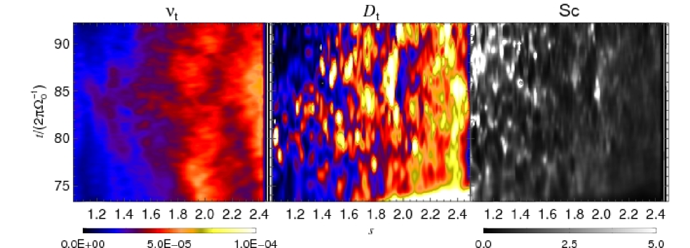
Figure 17: Azimuthally and vertically averaged turbulent viscosity $\nu_{t}$, turbulent diffusion $D_{t}$ and the resulting Schmidt number Sc as a function of radial position and time for model A. Time is quoted in orbits at $s_{0}$. Viscosity and diffusion are shown in the same units and color-code. Some localized overdensities in diffusion last for some orbits, while viscosity shows a smoother evolution in time. The quantities have approximately the same strength, as the Schmidt number is overall around unity, and seldom greater than 5.

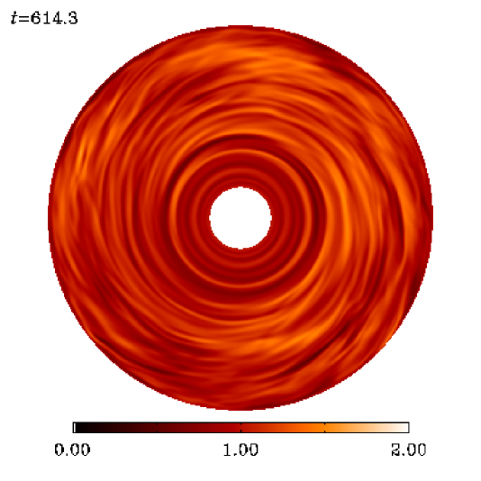
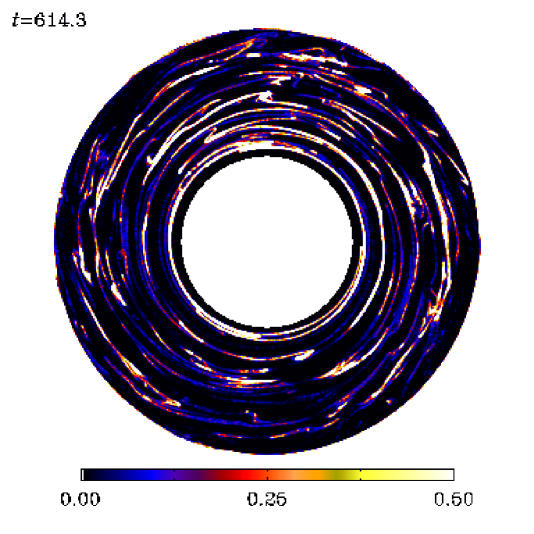
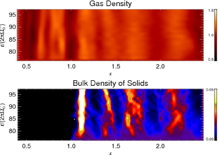
Figure 18: Density contours at midplane of the gas and solid phases of the disk (left and right panel, respectively). The snapshots were taken at 20 orbits at $s_{0}$ after the insertion of the particles. The color code for the solid phase is selected to represent 2 sigma (0.25) above the average bulk density of 0.03. The bright areas are saturated as the maximum density reaches as far as 85. A movie of this simulation can be found at http://www.astro.uu.se/$\sim$wlyra/planet.html. A correlation with gas density is seen, since the bright clumps of solids correspond to pressure maxima, i.e, areas of high gas density.

Figure 19: Maximum bulk density of solids, in units of the mean gas density as a function of time for model A. Time is quoted in orbits at $s_{0}$. The maximum density rises as the particles sediment towards the midplane. After the sedimentation that lasts for four orbits, the particles are coupled with the gas and trapping in transient gas high pressures raise their maximum density well above average. The maximum density is usually around 30, but between orbits 12 and 13, it reached values as high as 85.

6 Summary and conclusions

We have considered MHD models of global Keplerian disks in Cartesian grids. These disk-in-a-box models are able to develop and sustain MHD turbulence, in good agreement with published results achieved with cylindrical codes and shearing boxes. In this first article of the series, we investigated the dependence of the MRI with disk scale height and the dynamics of solid boulders in the global hydromagnetic turbulence.

As a numerical solver we have used the Pencil Code. This finite-difference code solves the non-conservative form of the dynamical equations using sixth-order spatial derivatives, achieving spatial resolution that approaches that of spectral methods. The numerical scheme is stabilized by using hyperdissipation and shock dissipation terms, which enter as free parameters in the dynamical equations. The effect of hyperdissipation is to quench unstable modes in the small scales of the grid, while affecting the large scale motion as little as possible, whereas shock dissipation is invoked to smear out large divergences in the flow field. We choose these parameters by performing series of 2D gap opening simulations with a Jupiter mass planet and comparing them with a higher resolution calculation without explicit dissipative terms.

We find evidence that the turbulence generated by the magnetorotational instability grows with the thermal pressure. The turbulent stresses depend on thermal pressure obeying a power law of $0.24\pm 0.03$, compatible with the value of $0.25$ found in shearing box calculations by Sano et al. (2004). We extend this result to a global disk showing that the rise in pressure increases the turbulent stresses, thus raising the angular momentum transport (and therefore the mass accretion rate) although the alpha viscosity value drops.

We also notice two curious effects. First, the dominance of the radial component of the turbulent kinetic energy increases with temperature. The percentage of the total kinetic energy stored in the radial component is 40% for the cold model A, and 60% for the hotter model C. Second, the ratio of stresses $-M^{s\phi}/R^{s\phi}$ diminished with increasing temperature. It is 5 for model A, and just 1.3 for model C. The same is seen in the model without inner boundary, where the ratio is 6.5 for model A2 and very close to 1 for model C2. This effect is unexpected since it is believed that the shear parameter alone controls the ratio of stresses (Pessah et al. 2006, Ogilvie & Pringle 1996). From the shearing box data of Sano et al. (2004) the stress ratio seems to be constant with temperature.

One explanation could be that, according to Eq. 12, the angular velocity is sub-Keplerian and the increasing effects of pressure from the colder to the hotter models modifies the shear. Quantitatively, however, one sees that the pressure correction is too small to account for the decrease in the stress ratio and, more importantly, would have the opposite effect. According to the linearized equations for the evolution of the turbulent fluctuations, the Maxwell stress couples with shear $q\Omega$, and the Reynolds stress couples with the large scale vorticity $w=(2-q)\Omega$ (Balbus & Hawley 1998), where $q=-\partial\ln\Omega/\partial\ln r$ is the shear rate. The pressure-corrected angular velocity of the gas can be approximated from Eq. (12) as

$$\Omega\simeq\Omega_{\rm K}(1-\eta)\,,$$ (25)

where $\eta=(1/2)(\partial\ln P/\partial\ln r)(H/s)^{2}>0$ is a parameter often used to parameterize the strength of the global pressure gradient (see e.g. Nakagawa et al. 1986). Typical values of $\eta$ lie between $0.001$ and $0.1$.

The reduction of both the angular frequency and shear rate should reduce the Maxwell stress. Our simulations show the opposite, with the Maxwell stress increasing as the pressure is raised. Regarding the stress ratio, reducing the shear increases this quantity since the Reynolds stress falls faster than the Maxwell stress due to the stabilizing effect of the growing vorticity (Abramowicz et al., 1996). Once again, we see the opposite effect.

As most of the analysis of turbulent thin accretion disks have focused on locally isothermal simulations using $c_{s}\approx 0.05$, changing the field configuration while keeping the temperature constant, such behavior has been largely overlooked. Although the disk temperatures considered in this case are quite extreme for disks around T-Tauri stars, circumplanetary disks are thought to be rather thick (Klahr & Kley 2006) and therefore the evolution of the MRI in such disks is expected to be more similar to the hotter cases considered in this paper (models CEG) than the colder ones.

We investigated the effect of an inner boundary in the evolution and outcome of the turbulence. By using a Cartesian grid, an inner boundary can be discarded provided we smooth the gravitational potential to avoid a singularity in the flow. Models without an inner boundary do not show the spurious build-up of magnetic pressure and Reynolds stress seen in the models with boundaries, while the global stresses and alpha viscosities are similar in the two cases.

In treating the solids, we make use of a large number of particles, which allows us to effectively map the particles back into the grid as a density field without using fluid approaches. We monitor the settling of the particles toward the midplane and the formation of a sedimentary layer when the solids are subject to gas drag and the gravity from the central object. The effective diffusion provided by the turbulence prevents further settling of solids, in accordance with the results of Johansen & Klahr (2005). By having the global disk perspective, we could measure the radial dependence of the diffusion scale height of the solid component. The measured scale heights imply turbulent vertical diffusion coefficients with globally averaged Schmidt numbers of 1.0$\pm$0.2 for model A ($\alpha\approx 10^{-3}$) and 0.78$\pm$0.06 for model D ($\alpha\approx 10^{-1}$).

We conclude that the models presented in this first paper of the series are capable of sustaining turbulence and are adequately suited for further studies of planet formation. Future papers will present studies of thermodynamics and radiative transfer in the evolution of the turbulent stresses, planet-planet and planet-disk interaction, the effect of stratification and the dynamics of dead zones.

Appendix A Anisotropic hyperdissipation

Hyperdissipation is used to quench unstable modes at the grid scale, therefore being intrinsically resolution-dependent. Because of this, isotropic dissipation only gives equal dissipation in all spatial directions if $\Delta x=\Delta y=\Delta z$, i.e., if the cells are cubic. For non-cubic cells, anisotropic dissipation is required as different directions may be better/worse sampled, thus needing less/more numerical smoothing. Such a generalization is straightforward. We notice that hyperdiffusion works as a conservative term in the continuity equation such that

$$f_{D}(\rho)={\bm{\nabla}}\cdot{\bm{\mathcal{J}}},$$ (26)

where ${\bm{\mathcal{J}}}=D_{3}{\bm{\nabla}}^{5}\rho$ is the mass flux due to hyperdiffusion. For simplicity, we will drop the subscripts “3” from the coefficients hereafter. This formulation reduces to the usual sixth-order hyperdiffusion under the condition that $D$ is constant. Generalizing it to three dimensions simply involves replacing this mass flow by

$${\bm{\mathcal{J}}}=\left(D_{x}\frac{{\partial{}}^{5}\rho}{{\partial x}^{5}},D_{y}\frac{{\partial{}}^{5}\rho}{{\partial y}^{5}},D_{z}\frac{{\partial{}}^{5}\rho}{{\partial z}^{5}}\right),$$

so that different diffusion operates in different directions. Since $D_{x}$, $D_{y}$ and $D_{z}$ are constants, the divergent of this vector is

$${\bm{\nabla}}\cdot{\bm{\mathcal{J}}}=D_{x}\frac{{\partial{}}^{6}\rho}{{\partial x}^{6}}+D_{y}\frac{{\partial{}}^{6}\rho}{{\partial y}^{6}}+D_{z}\frac{{\partial{}}^{6}\rho}{{\partial z}^{6}}.$$

The formulation for resistivity is strictly the same. For viscosity it also assumes the same form if we consider a simple $n$th order rate of strain tensor operator $S^{(n)}_{ij}=\partial{}^{n}_{j}{u_{i}}$.

Appendix B Shocks

Shock viscosity is taken to be proportional to positive flow convergence, maximum over three zones, and smoothed to second order,

$$\zeta_{\nu}=\nu_{\rm sh}\left<\max_{3}[(-{\bm{\nabla}}\cdot{\bm{u}})_{+}]\right>{\left[\min(\Delta x,\ \Delta y,\Delta z)\right]}^{2},$$ (27)

where $\nu_{\rm sh}$ is a constant defining the strength of the shock viscosity, usually around unity. We refer to it as the shock viscosity coefficient (Haugen et al. 2004). In the equation of motion it takes the form of a bulk viscosity so that now the stress tensor contains

$$\tau_{ij}=[...]+\rho\zeta_{\nu}\delta_{ij}{\bm{\nabla}}\cdot{\bm{u}},$$ (28)

where […] refers to the (hyper) viscous terms described in Appendix A. The acceleration due to shock viscosity is therefore

$$f_{\nu}({\bm{u}},\rho) = \rho^{-1}{\bm{\nabla}}\cdot\tau$$

$$= \zeta_{\nu}\left[{\bm{\nabla}}({\bm{\nabla}}\cdot{\bm{u}})+\left({\bm{\nabla}}\ln\rho+{\bm{\nabla}}\ln\zeta_{\nu}\right){\bm{\nabla}}\cdot{\bm{u}}\right].$$

Such a viscosity scheme ensures that energy is dissipated in regions of the flow where shocks occur, whereas more quiescent regions are left untouched. The formulations for shock diffusion and shock resistivity are similar, yielding

$$f_{D}(\rho)=\zeta_{D}\left(\nabla^{2}\rho+{\bm{\nabla}}\ln\zeta_{D}\cdot{\bm{\nabla}}\rho\right),$$ (30)

and

$$f_{\eta}({\bm{A}})=\zeta_{\eta}\left(\nabla^{2}{\bm{A}}+{\bm{\nabla}}\ln\zeta_{\eta}{\bm{\nabla}}\cdot{\bm{A}}\right),$$ (31)

where $\zeta_{D}$ and $\zeta_{\eta}$ are analogous to $\zeta_{\nu}$ in Eq. (27), containing their respective shock diffusion and shock resistivity coefficients $D_{\rm sh}$ and $\eta_{\rm sh}$.

References

- (1) Abramowicz, M., 1996, in Physics of Accretion Disks, edited by S. Kato, S. Inagaki, S. Mineshige, and J. Fukue (Gordon and Breach, Amsterdam), p. 1
- (2) D’Angelo, G., Henning, T., & Kley, W., 2003, ApJ, 599, 548
- (3) Armitage, P. J., 1998, ApJ, 501, 189
- (4) Armitage, P. J., Reynolds, C. S., & Chiang, J., 2001, ApJ, 548, 868
- (5) Balbus, S.A., & Hawley, J.F., 1998, RvMP, 70, 1
- (6) Balbus, S.A., & Hawley, J.F., 1992, ApJ, 400, 610
- (7) Balbus, S.A., & Hawley, J.F., 1991, ApJ, 376, 214
- (8) Barge, P., Sommeria, J., 1995, A&A, 295, 1
- (9) Brandenburg, A, Nordlund, Å, Stein, R.F., & Torkelsson, U., 1995, ApJ, 446, 741
- (10) Chandrasekhar, S., 1960, Proc. Nat. Acad. Sci., 46, 253
- (11) -. 1961, Hydrodynamic and Hydromagnetic Stability (Oxford: Clarendon), 384
- (12) Dobler, W., Stix, M., & Brandenburg, A, 2006, ApJ, 638, 336
- (13) Dobler, W., private communication
- (14) Dubrulle, B., Morfill, G., & Sterzik, M., 1995, 114, 237
- (15) Freytag, B., Steffen, M., & Dorch, B., 2002, AN, 323, 213
- (16) Fromang, S., & Nelson, R. P., 2006, A&A, 457, 343
- (17) Fromang, S., & Nelson, R. P., 2005, MNRAS, 364, 81
- (18) Gammie, C. F., 1996, ApJ, 457, 355
- (19) Goldreich, P., & Ward, W. R. 1973, ApJ, 183, 1051
- (20) Haugen, N.E.L., & Brandenburg, A.,2004,PhRvE,70b,6405
- (21) Haugen, N.E.L., Brandenburg, A., & Mee, A. J., MNRAS, 353, 947
- (22) Hawley, J.F., 2000, ApJ, 528, 462
- (23) Hawley, J.F. & Balbus, S.A., 1991, ApJ, 376, 223
- (24) Hawley, J. F., Gammie, C. F., & Balbus, S. A. 1995, ApJ, 440, 742
- (25) Hawley, J.F., 2001, ApJ, 554, 534
- (26) Johansen, A., Oishi, J. S., Mac Low, M.-M., Klahr, H., Henning, Th., & Youdin, A., 2007, Nature, 448, 1022
- (27) Johansen, A., Klahr, H., & Henning, T. 2006, ApJ, 636, 1121
- (28) Johansen, A., & Klahr, H., 2005, ApJ, 634, 1353
- (29) Kant I., 1755, Universal Natural History and Theories of the Heaven
- (30) Klahr, H., & Kley, W., 2006, A&A, 445, 747
- (31) Klahr, H., & Lin, D. N. C., 2001, ApJ, 554, 1095
- (32) Kwok, S., 1975, ApJ, 198, 583
- (33) Laplace P.S., 1796, Mécanique Céleste
- (34) Lin, D.N.C., & Papaloizou, J., 1986, ApJ, 309, 846
- (35) Lucas, P.W., & Roche, P.F., 2000, MNRAS, 314, 858
- (36) Marcy, G.W., & Butler, R.P., 1996, ApJ, 464, 147
- (37) Masset, F., D’Angelo, G., & Kley, W., 2006, ApJ, 652, 730
- (38) Mayor, M., & Queloz, D., 1995, Nature, 378, 355
- (39) Miller, K. A., & Stone, J. M., 2000, ApJ, 534, 398
- (40) Mizuno H., 1980, P.T.Ph., 64, 2
- (41) Nakagawa Y., Sekiya M., & Hayashi C., 1986, Icarus, 67, 375
- (42) Nelson, R.P., 2005, A&A, 443, 1067
- (43) van Noort, M., Hubeny, I., Lanz, T., 2002, ApJ, 568, 1066
- (44) Ogilvie, G. I., Pringle, J. E., 1996, MNRAS, 279, 152O
- (45) Oishi, J. S., Mac Low, M.-M., & Menou, K., 2007, astro-ph/0702549
- (46) Paardekooper, S.-J., 2007, A&A, 462, 355
- (47) Paardekooper, S.-J. & Mellema, G., 2006, A&A, 459, 17
- (48) Papaloizou, J. C. B., Nelson, R. P., 2003, MNRAS, 339, 983
- (49) Pessah, M.E., Chan, C.-K., & Psaltis, D., 2006, MNRAS, 372, 183
- (50) Pollack, J.B, Hubickyj, O., Bodenheimer, P., Lissauer, J. J., Podolak, M., & Greenzweig, Y., 1996, Icarus, 124, 62
- (51) Pringle, J.E., 1981, ARAA, 19, 137
- (52) von Rekowski, B., & Piskunov, N., 2006, AN, 327, 340
- (53) Rivera, E.J., Lissauer, J.J., Butler, R.P., Marcy, G.W., Vogt, S.S., Fischer, D.A., Brown, T.M., Laughlin, G., & Henry, G.W., 2005, ApJ, 634, 625
- (54) Safronov, V.S., 1969, QB, 981, 26
- (55) Sano, T., Inutsuka, S.-I., Turner, N.J., & Stone, J.M., 2004, ApJ, 605, 321
- (56) Shakura, N.I., & Sunyaev, R.A., 1973, A&A, 24, 37
- (57) Sicilia-Aguilar, A., Hartmann, L.W., Briceño, C., Muzerolle, J., & Calvet, N., 2004, AJ, 128, 805
- (58) de Val-Borro, M., Edgar, R.G., Artymowicz, P., Ciecielag, P., Cresswell, P., D’Angelo, G., Delgado-Donate, E.J., Dirksen, G., Fromang, S., Gawryszczak, A., Klahr, H., Kley, W., Lyra, W., Masset, F., Mellema, G., Nelson, R., Paardekooper, S.-J., Peplinski, A., Pierens, A., Plewa, T., Rice, K., Schäfer, C., & Speith, R., 2006, MNRAS
- (59) Velikhov, E. P., 1959, Soviet Phys. - JETP, 36, 1398
- (60) Ward, W. R., 1981, Icarus, 47, 234
- (61) Ward, W.R., & Hourigan, K., 1989, ApJ, 347, 490
- (62) Weidenschilling, S. J. 1977, MNRAS, 180, 5
- (63) Wolszczan, A., & Frail, D.A., 1992, Nature, 355, 145
- (64) Youdin, A., & Johansen, A., 2007, ApJ, 662, 613
- (65) Youdin, A. N., Shu, F. H., 2002, ApJ, 580, 494