Solving ill-conditioned linear algebraic systems bythe dynamical systems method (DSM)

Abstract

An iterative scheme for the Dynamical Systems Method (DSM) is given such that one does not have to solve the Cauchy problem occuring in the application of the DSM for solving ill-conditioned linear algebraic systems. The novelty of the algorithm is that the algorithm does not have to find the regularization parameter $a$ by solving a nonlinear equation. Numerical experiments show that DSM competes favorably with the Variational Regularization.

Keywords: ill-posed problems, ill-conditioned linear algebraic systems, dynamical systems method (DSM).

AMS subject classification: 65F10, 65F22.

1 Introduction

Consider a linear operator equation of the form

$$F(u)=Au-f=0,\quad u\in H,$$ (1)

where $H$ is a Hilbert space and $A$ is a linear operator in $H$ which is not necessarily bounded but closed and densely defined. To solve this equation we apply the Dynamical Systems Method (DSM) introduced in [6]:

$$u^{\prime}=-u+(T+a(s))^{-1}A^{*}f,\quad u(0)=u_{0},$$ (2)

where $T:=A^{*}A$ and $a(t)>0$ is a nonincreasing function such that $a(t)\to 0$ as $t\to\infty$. The unique solution to (2) is given by

$$u(t)=u_{0}e^{-t}+e^{-t}\int_{0}^{t}e^{s}(T+a(s))^{-1}A^{*}fds.$$ (3)

The DSM consists of solving problem (2) with a chosen $a(t)$ and $u_{0}$ and finding a stopping time $t_{\delta}$ so that $u(t_{\delta})$ approximates the solution $y$ to problem (1) of minimal norm. Different choices of $a(t)$ generate different methods of solving equation (1). These methods have different accuracy and different computation time. Thus, in order to get an efficient implementation of the DSM, we need to study the choice of $a(t)$ and of the stopping time $t_{\delta}$. Since the solution to (1) can be presented in the form of an integral, the question arises: how can one compute the integral efficiently? The integrand of the solution is used also in the Variational Regularization (VR) method. The choice of the stopping time $t_{\delta}$ will be done by a discrepancy-type principle for DSM. However, choosing $a(t)$ so that the method will be accurate and the computation time is small is not a trivial task.

This paper deals with the following questions:

1. How can one choose $a(t)$ so that the DSM is fast and accurate?

2. Does the DSM compete favorably with the VR in computation time?

3. Is the DSM comparable with the VR in accuracy?

2 Construction of method

2.1 An iterative scheme

Let us discuss a choice of $a(t)$ which allows one to solve problem (2) or to calculate the integral (3) without using any numerical method for solving initial-value problem for ordinary differential equations (ODE). In fact, using a monotonically decreasing $a(t)$ with one of the best numerical methods for nonstiff ODE, such as DOPRI45, is more expensive computationally than using a step function $\tilde{a}(t)$, approximating $a(t)$, but brings no improvement in the accuracy of the solution to our problems compared to the numerical solution of our problems given in Section 3.1.2.

Necessary conditions for the function $a(t)$ are: $a(s)$ is a nonincreasing function and $\lim_{s\to\infty}a(s)=0$ (see [6]). Thus, our choice of $a(t)$ must satisfy these conditions. Consider a step function $\tilde{a}(t)$, approximating $a(t)$, defined as follows:

$$\tilde{a}(t)=a_{n},\quad t_{n}\leq t<t_{n+1},$$

the number $t_{n}$ are chosen later. For this $\tilde{a}(t)$, $u_{n}=u(t_{n})$ can be computed by the formula:

$$u_{n}=u_{0}e^{-t_{n}}+e^{-t_{n}}\sum_{i=1}^{n}(e^{t_{i}}-e^{t_{i-1}})(T+a_{i-1})^{-1}A^{*}f_{\delta}.$$

This leads to the following iterative formula:

$$u_{n+1}=e^{-h_{n}}u_{n}+(1-e^{-h_{n}})\big{(}T+a_{n}\big{)}^{-1}A^{*}f_{\delta},\quad h_{n}=t_{n+1}-t_{n}.$$ (4)

Thus, $u_{n}$ can be obtained iteratively if $u_{0}$ , $a(t)$ and $t_{n}$ are known.

The questions are:

1. For a given $a(t)$, how can we choose $t_{n}$ or $h_{n}$ so that the DSM works efficiently?

2. With $a_{n}=a(t_{n})$ where $a(t)$ is a continuous function, does the iterative scheme compete favorably with the DSM version in which $u(t)$ is solved by some numerical methods such as Runge-Kutta methods using $a(t)$?

In our experiments, $a_{n}=a(t_{n})$ where $a(t)=\frac{a_{0}}{1+t}$ where $a_{0}>0$ is a constant which will be chosen later, as suggested in [6], with $t_{n}$ chosen so that $t_{n+1}-t_{n}=h_{n}$, $h_{n}=q^{n}$, where $1\leq q\leq 2$. For this choice, if $q>1$ then the solution $u_{n}$ at the $n$-th step depends mainly on $\big{(}T+a_{n}\big{)}^{-1}A^{*}f_{\delta}$ since $e^{-h_{n}}$ is very small when $n$ is large.

Note that $a_{n}$ decays exponentially fast when $n\to\infty$ if $q>1$. A question arises: how does one choose $q$ so that the method is fast and accurate? This question will be discussed in Section 3.

ALGORITHM 2.1 demonstrates the use of the iterative formula (4) and a relaxed discrepancy principle described below for finding $u$ given $a_{0}$, $A$, $f_{\delta}$ and $\delta$.

In order to improve the speed of the algorithm, we use a relaxed discrepancy principle: at each iteration one checks if

$$0.9\delta\leq\|Au_{n}-f_{\delta}\|\leq 1.001\delta.$$ (5)

As we shall see later, $a_{0}$ is chosen so that the condition (7) (see below) is satisfied. Thus, if $u_{0}=T_{a_{0}}^{-1}A^{*}f_{\delta}$, where $T_{a}:=T+a$, then $\delta<\|Au_{0}-f_{\delta}\|$. Let $t_{n}$ be the first time such that $\|Au_{n}-f_{\delta}\|\leq 1.001\delta$. If (6) is satisfied, then one stops calculations. If $\|Au_{n}-f_{\delta}\|<0.9\delta$, then one takes a smaller step-size and recomputes $u_{n}$. If this happens, we do not increase $h_{n}$, that is, we do not multiply $h_{n}$ by $q$ in the following steps. One repeats this procedure until condition (6) is satisfied.

Algorithm 1: DSM$(A,f_{\delta},\delta)$ $q:=2$; $g_{\delta}:=A^{*}f_{\delta}$;   $T:=A^{*}A$; $itermax:=30$;   $u=(T+a_{0})^{-1}g_{\delta}$; $i:=0$;   $t=1$;   $h:=1$;   $halve:=0$; while $(1.001\delta<\|Au-f_{\delta}\|)$ and $(i<itermax)$ do $i:=i+1$;   $t=t+h$;   $a=a_{0}/t$; $v:=(T+aI)^{-1}g_{\delta}$; $\tilde{u}=e^{-h}u+(1-e^{-h})v$; if $0.9\delta<\|A\tilde{u}-f_{\delta}\|$ then $u:=\tilde{u}$; if $halve=0$ then $h:=hq$;   end; elseif $t:=t-h$;   $h:=h/2$;   $halve=1$; endif endwhile

In order to improve the speed of the algorithm, we use a relaxed discrepancy principle: at each iteration one checks if

$$0.9\delta\leq\|Au_{n}-f_{\delta}\|\leq 1.001\delta.$$ (6)

As we shall see later, $a_{0}$ is chosen so that the condition (7) (see below) is satisfied. Thus, if $u_{0}=T_{a_{0}}^{-1}A^{*}f_{\delta}$, where $T_{a}:=T+a$, then $\delta<\|Au_{0}-f_{\delta}\|$. Let $t_{n}$ be the first time such that $\|Au_{n}-f_{\delta}\|\leq 1.001\delta$. If (6) is satisfied, then one stops calculations. If $\|Au_{n}-f_{\delta}\|<0.9\delta$, then one takes a smaller step-size and recomputes $u_{n}$. If this happens, we do not increase $h_{n}$, that is, we do not multiply $h_{n}$ by $q$ in the following steps. One repeats this procedure until condition (6) is satisfied.

2.2 On the choice of $a_{0}$

From numerical experiments with ill-conditioned linear algebraic systems (las) of the form $Au=f_{\delta}$, it follows that the regularization parameter $a_{M}$, obtained from the discrepancy principle $\|Au_{a_{M}}-f_{\delta}\|=\delta$, where $u_{a_{M}}=T_{a_{M}}^{-1}A^{*}f_{\delta}$, is often close to the optimal value $a_{op}$, i.e., the value minimizing the quantity:

$$\|u_{a_{op}}-y\|=\inf_{a}\|u_{a}-y\|,\quad u_{a}=T_{a}^{-1}Af_{\delta}.$$

The letter $M$ in $a_{M}$ stands for Morozov, who suggested to choose $c=1$ in the disrepancy principle.

If $a_{0}$ is chosen smaller than $a_{op}$, the method may converge poorly. Since $a_{M}$ is close to $a_{op}$, only those $a$ for which $\|AT_{a}^{-1}A^{*}f_{\delta}-f_{\delta}\|=c\delta$ with $c$ ’close’ to $1$ yield accurate approximations to the solution $y$. Also, if $a_{0}$ is chosen much greater than $a_{op}$, then the information obtained from the starting steps of the iterative process (4) is not valuable because when $a_{0}$ is far from $a_{op}$, the error $\|u_{a_{0}}-y\|$ is much bigger than $\|u_{a_{op}}-y\|$. If $a_{0}$ is much bigger than $a_{op}$, a lot of time will be spent until $a(t_{n})$ becomes close to $a_{op}$. In order to increase the speed of computation, $a_{0}$ should be chosen so that it is close to $a_{op}$ and greater than $a_{op}$. Since $a_{op}$ is not known and is often close to $a_{M}$, we choose $a_{0}$ from the condition:

$$\delta<\|Au_{a_{0}}-f_{\delta}\|<2\delta.$$ (7)

For this choice, $a_{0}$ is ’close’ to and greater than $a_{M}$. Since there are many $a_{0}$ satisfying this condition, it is not difficult to find one of them.

In the implementation of the VR using discrepancy principle with Morozov’s suggestion $c=1$, if one wants to use the Newton method for finding the regularization parameter, one also has to choose the starting value $a_{0}$ so that the iteration process converges, because the Newton method, in general, converges only locally. If this value is close to and greater than $a_{M}$, it can also be used as the initial value of $a_{0}=a(t)|_{t=0}$ for the DSM.

In our numerical experiments, with a guess $a_{0}=\frac{1}{3}\max\lambda_{i}(A^{*}A)\delta_{rel}$ for $a(0)$, we find $a_{0}$ such that $\delta<\|Au_{a_{0}}-f_{\delta}\|<2\delta$. Here, $\delta_{rel}$ stands for the relative error, i.e., $\delta_{rel}=\frac{\delta}{\|f\|}$. The factor $\frac{1}{3}$ is introduced here in order to reduce the cost for finding $a_{0}$, because $a_{0}$, which satisfies (7), is often less than $\max\lambda_{i}(A^{*}A)\delta_{rel}$. The idea for this choice is based on the fact that the spectrum of the matrix $\frac{1}{\max\lambda_{i}(A^{*}A)}A^{*}A$ is contained in $[0,1]$.

Note that ones has

$$a_{M}\leq\frac{\delta\|A\|^{2}}{\|f_{\delta}\|-\delta}.$$

Indeed,

$$\|f_{\delta}\|-\delta =\|f_{\delta}\|-\|Au_{a_{M}}-f_{\delta}\|\leq\|Au_{a_{M}}\|.$$

Since $A^{*}Au_{a_{M}}+a_{M}u_{a_{M}}=A^{*}f_{\delta}$, one has $a_{M}Au_{a_{M}}=AA^{*}(f_{\delta}-Au_{a_{M}})$. Thus,

$$\|f_{\delta}\|-\delta\|\leq\|Au_{a_{M}}\|=\frac{1}{a_{M}}\|AA^{*}(f_{\delta}-Au_{a_{M}})\|\leq\frac{\|A\|^{2}}{a_{M}}\delta.$$

Similar estimate one can find in [5, p. 53], where $a_{0}=\frac{\delta\|A\|^{2}}{\|f_{\delta}\|-\delta}$ is suggested as a starting value for Newton’s method to determine $a_{M}$ on the basis that it is an upper bound for $a_{M}$. Note that $\frac{\delta\|A\|^{2}}{\|f_{\delta}\|-\delta}\approx\delta_{rel}\|A\|^{2}=\max\lambda_{i}(A^{*}A)\delta_{rel}$. However, in practice Newton’s method does not necessarily converge with this starting value. If this happens, a smaller starting value $a_{1}:=\frac{a_{0}}{2}$ is used to restart the Newton’s method.

In general, our initial choice for $a_{0}$ may not satisfy (7). Iterations for finding $a_{0}$ to satisfy (7) are done as follows:

1. If $\frac{\|Au_{a_{0}}-f_{\delta}\|}{\delta}=c>3$, then one takes $a_{1}:=\frac{a_{0}}{2(c-1)}$ as the next guess and checks if the condition (7) is satisfied. If $2<c\leq 3$ then one takes $a_{1}:=a_{0}/3$.

2. If $\frac{\|Au_{a_{0}}-f_{\delta}\|}{\delta}=c<1$, then $a_{1}:=3a_{0}$ is used as the next guess.

3. After $a_{0}$ is updated, one checks if (7) is satisfied. If (7) is not satisfied, one repeats steps 1 and 2 until one finds $a_{0}$ satisfying condition (7) (see ALGORITHM 2.2).

Algorithm 2: find-$a_{0}$ $a_{0}:=\frac{1}{3}\|A\|^{2}\delta_{rel}$; $c:=\|Au_{a_{0}}-f_{\delta}\|/\delta$; while $(2<c)$ or $(c<1)$ do if $3<c$ then $a_{0}:=0.5a_{0}/(c-1)$; elseif $(2<c\leq 3)$ then $a_{0}:=a_{0}/3$; else $a_{0}:=3a_{0}\kern 2.0pt;~{}~{}~{}\ignorespaces$ end $u_{a_{0}}:=(A^{*}A+a_{0})^{-1}A^{*}f_{\delta}$; $c:=\|Au_{a_{0}}-f_{\delta}\|/\delta$; endwhile

The above strategy is based on the fact that the function

$$\phi(a)=\|A(T+a)^{-1}A^{*}f_{\delta}-f_{\delta}\|$$

is a monotonically decreasing function of $a$, $a>0$. In looking for $a_{0}$, satisfying (7), when our guess $a_{0}\gg a_{M}>0$ or $\|Au_{a_{0}}-f_{\delta}\|\gg\delta$, one uses an approximation

$$\phi(x) \approx\phi(a_{0})+(x-a_{0})\frac{\phi(a_{0})-\phi(a_{M})}{a_{0}-a_{M}}$$

$$\approx\phi(a_{0})+(x-a_{0})\frac{\phi(a_{0})-\phi(a_{M})}{a_{0}}=:\varphi(x).$$

Note that $\phi(a_{0})$ and $a_{0}$ are known. We are looking for $x$ such that $\delta<\varphi(x)<2\delta$. Thus, if $a_{1}$ is such that $\delta<\varphi(a_{1})<2\delta$ and if $2\delta<\phi(a_{0})$, then

$$(\phi(a_{0})-2\delta)\frac{a_{0}}{\phi(a_{0})-\delta}<a_{0}-a_{1}<(\phi(a_{0})-\delta)\frac{a_{0}}{\phi(a_{0})-\delta}.$$

Hence, we choose $a_{1}$ such that

$$a_{0}-a_{1}=(\phi(a_{0})-1.5\delta)\frac{a_{0}}{\phi(a_{0})-\delta},$$

so

$$a_{1}=a_{0}\frac{0.5\delta}{\phi(a_{0})-\delta}.$$

Although this is a very rough approximation, it works well in practice. It often takes 1 to 3 steps to get an $a_{0}$ satisfying (7). That is why we have a factor $\frac{0.5}{c-1}$ in the first case. Overall, it is easier to look for $a_{0}$ satisfying (7) than to look for $a_{0}$ for which the Newton’s method converges. Indeed, the Newton’s scheme for solving $a_{M}$ does not necessarily converge with $a_{0}$ found from condition (7).

3 Numerical experiments

In this section, we compare DSM with VR_i and VR_n. In all methods, we begin with the guess $a_{0}=\frac{1}{3}\|A\|^{2}\delta_{rel}$ and use the ALGORITHM 2.2 to find $a_{0}$ satisfying condition (7). In our experiments, the computation cost for this step is very low. Indeed, it only takes 1 or 2 iterations to get $a_{0}$. By VR_i we denote the VR obtained by using $a=a_{0}$, the intial value for $a(t)$ in DSM, and by VR_n we denote the VR with $a=a_{M}$, found from the VR discrepancy principle with $c=1$ by using Quasi-Newton’s method with the initial guess $a=a_{0}$. Quasi-Newton’s method is chosen instead of Newton’s method in order to reduce the computation cost. In all experiments we compare these methods in accuracy and with respect to the parameter $N_{linsol}$, which is the number of times for solving the linear system $T_{a}u=A^{*}f_{\delta}$ for $u$. Note that solving these linear systems is the main cost in these methods.

In this section, besides comparing the DSM with the VR for linear algebraic systems with Hilbert matrices, we also carry out experiments with other linear algebraic systems given in the Regularization package in [4]. These linear systems are obtained as a part of numerical solutions to some integral equations. Here, we only focus on the numerical methods for solving linear algebraic systems, not on solving these integral equations. Therefore, we use these linear algebraic systems to test our methods for solving stably these systems.

3.1 Linear algebraic systems with Hilbert matrices

Consider a linear algebraic system

$$H_{n}u=f_{\delta},$$ (8)

where

$$f_{\delta}=f+e,\quad f=H_{n}x,\quad H_{n}=\begin{bmatrix}1&\frac{1}{2}&\cdots&\frac{1}{n}\\ \frac{1}{2}&\frac{1}{3}&\cdots&\frac{1}{n+1}\\ \vdots&\vdots&\ddots&\vdots\\ \frac{1}{n}&\frac{1}{n+1}&\cdots&\frac{1}{2n-1}\end{bmatrix},$$

and $e\in\mathbb{R}^{n}$ is a random normally distributed vector such that $\|e\|_{2}\leq\delta_{rel}\|f\|_{2}$. The Hilbert matrix $H_{n}$ is well-known for having a very large condition number when $n$ is large. If $n$ is sufficiently large, the system is severely ill-conditioned.

3.1.1 The condition numbers of Hilbert matrices

It is impossible to calculate the condition number of $H_{n}$ by computing the ratio of the largest and the smallest eigenvalues of $H_{n}$ because for large $n$ the smallest eigenvalue of $H_{n}$ is smaller than $10^{-16}$. Note that singular values of $H_{n}$ are its eigenvalues since $H_{n}$ is selfadjoint and positive definite. Due to the limitation of machine precision, every value smaller than $10^{-16}$ is understood as 0. That is why if we use the function cond provided by MATLAB, the condition number of $H_{n}$ for $n\geq 20$ is about $10^{16}\times\max|\lambda_{i}(H_{n})|$. Since the largest eigenvalue of $H_{n}$ grows very slowly, the condition numbers of $H_{n}$ for $n\geq 20$ are all about $10^{20}$, while, in fact, the condition number of $H_{100}$ computed by the formula, given below, is about $10^{150}$ (see Table 1). In general, computing condition numbers of strongly ill-conditioned matrices is an open problem. The function cond, provided by MATLAB, is not always reliable for computing the condition number of ill-condition matrices. Fortunately, there is an analytic formula for the inverse of $H_{n}$. Indeed, one has (see [2]) $H_{n}^{-1}=(h_{ij})_{i,j=1}^{n}$, where

$$h_{ij}=(-1)^{i+j}(i+j-1)\dbinom{n+i-1}{n-j}\dbinom{n+j-1}{n-i}\dbinom{i+j-2}{i-1}^{2}.$$

Thus, the condition number of the Hilbert matrix can be computed by the formula:

$$cond(H_{n})=\|H_{n}\|\|H_{n}^{-1}\|.$$

Here $cond(H_{n})$ stands for the condition number of the Hilbert matrix $H_{n}$ and $\|H_{n}\|$ and $\|H_{n}^{-1}\|$ are the largest eigenvalues of $H_{n}$ and $H_{n}^{-1}$, respectively. Although MATLAB can not compute values less than $10^{-16}$, it can compute values up to $10^{200}$. Therefore, it can compute $\|H_{n}^{-1}\|$ for $n$ up to 120. In MATLAB, the matrices $H_{n}$ and $H_{n}^{-1}$ can be obtained by the syntax: $H_{n}=\text{hilb}(n)$ and $H_{n}^{-1}=\text{invhilb}(n)$, respectively.

The condition numbers of Hilbert matrices, computed by the above formula, are given in Table 1.

Table 1: The condition number of Hilbert matrices.

$n$	20	40	60	80	100	120
$cond(H_{n})$	$2.5\times 10^{28}$	$7.7\times 10^{58}$	$2.7\times 10^{89}$	$9.9\times 10^{119}$	$3.8\times 10^{150}$	$1.5\times 10^{181}$

From Table 1 one can see that the computed condition numbers of the Hilbert matrix grow very fast as $n$ grows.

3.1.2 Continuous $a(t)$ compared to the step function $\tilde{a}(t)$

In this section, we compare the DSM, which is implemented by solving the Cauchy problem (2) with $a(t)$, and the iterative DSM implemented with $\tilde{a}(t)$ approximating $a(t)$ as described in Section 2.1. Both of them use the same $a_{0}$ which is found by ALGORITHM 2.2. The DSM using a numerical method to solve the Cauchy problem is implemented as follows:

1. One uses the DOPRI45 method which is an embedded pair consisting of a Runge-Kutta (RK) method of order 5 and another RK method of order 4 which is used to estimate the error in order to control the step sizes. The DOPRI45 is an explicit method which requires 6 right-hand side function evaluations at each step. Details about the coefficients and variable step size strategy can be found in [1, 3]. Using a variable step size helps to choose the best step sizes and improves the speed.

2. In solving (2), at the end of each step, one always checks the stopping rule, based on the discrepancy principle

   $$0.9\leq\|Au_{\delta}(t)-f_{\delta}\|\leq 1.001\delta.$$

   If this condition is satisfied, one stops and takes the solution at the final step $u(t_{n})$ as the solution to the linear algebraic system.

Table 2: Numerical results for Hilbert matrices for $\delta_{rel}=0.01$, $n=100$.

	DSM		DSM($q=1$)		DSM-DOPRI45
$n$	$N_{\text{linsol}}$	$\frac{\|u_{\delta}-y\|_{2}}{\|y\|_{2}}$	$N_{\text{linsol}}$	$\frac{\|u_{\delta}-y\|_{2}}{\|y\|_{2}}$	$N_{\text{linsol}}$	$\frac{\|u_{\delta}-y\|_{2}}{\|y\|_{2}}$
10	5	0.1222	10	0.1195	205	0.1223
20	5	0.1373	7	0.1537	145	0.1584
30	7	0.0945	20	0.1180	313	0.1197
40	5	0.2174	7	0.2278	151	0.2290
50	6	0.1620	14	0.1609	247	0.1609
60	6	0.1456	16	0.1478	253	0.1480
70	6	0.1436	13	0.1543	229	0.1554
80	6	0.1778	10	0.1969	181	0.1963
90	6	0.1531	13	0.1535	307	0.1547
100	7	0.1400	23	0.1522	355	0.1481

The DSM version implemented with the DOPRI45 method is denoted DSM-DOPRI45 while the other iterative version of DSM is denoted just by DSM.

Table 2 presents the numerical results with Hilbert matrices $H_{n}$ obtained by two versions of the DSM for $n=10,20,...,100$, $\delta_{rel}=0.01$, $x=(x_{1},...,x_{n})^{T}$, $x_{i}=\sqrt{2\frac{i-1}{100}\pi}$. From Table 2, as well as other numerical experiments, we found out that the accuracy obtained by the DSM-DOPRI45 is worse than that of the iterative DSM. Moreover, the computation time for the DSM-DOPRI45 is much greater than that for the iterative DSM. Also, using $h=$const or $q=1$ does not give more accurate solutions while requires more computation time.

The conclusion from this experiment as well as from other experiments is that the DSM with $q=2$ is much faster and often gives better results than the DSM with $q=1$ and the DSM-DOPRI45. Therefore, we choose the iterative DSM with $q=2$ to compare with the VR_n method.

3.1.3 DSM compared to VR

In this section, we test three methods: the DSM, the VR_i and the VR_n on linear algebraic systems with Hilbert matrices. The first linear system is obtained by taking $H_{100}$ and $x=(x_{1},...,x_{100})^{T}$, where $x_{i}=(\frac{i-1}{100})^{2}$. For the second problem we just change $x_{i}$ to $x_{i}=\sin(2\frac{i-1}{100}\pi)$. Numerical results for these systems are shown in Figure 1.

 

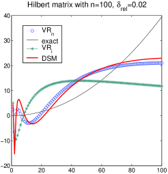
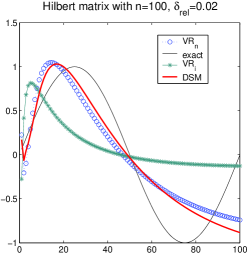
Figure 1: Plots of solutions obtained by the DSM and VR with the exact solution $x$, $x=(x_{i})_{i=1}^{100}$ when $x_{i}=(2\frac{i-1}{100}\pi)^{2}$ (left) and $x_{i}=\sin(2\frac{i-1}{100}\pi)$ (right) with $\delta_{rel}=0.02$.

Looking at Figure 1, one can see that with the same guess $a_{0}$, both the VR_n and DSM give better results than those of VR_i. As it can be seen from Figure 1, the numerical solutions obtained by the DSM in these tests are slightly more accurate than those of the VR_n.

Table 3 presents results with Hilbert matrices $H_{n}$ for $n=10,20,...,100$, $\delta_{rel}=0.01$, $x=(x_{1},...,x_{n})^{T}$, $x_{i}=\sqrt{2\frac{i-1}{100}\pi}$. Looking at this Table it is clear that the results obtained by the DSM are slightly more accurate than those by the VR_n even in the cases when the VR_n requires much more work than the DSM. In this example, we can conclude that the DSM is better than the VR_n in both accuracy and time of computation.

Table 3: Numerical results for Hilbert matrix $H_{n}$ for $\delta_{rel}=0.01$, $n=10,20,...,100$.

	DSM		VRi		VRn
n	$N_{\text{linsol}}$	$\frac{\|u_{\delta}-y\|_{2}}{\|y\|_{2}}$	$N_{\text{linsol}}$	$\frac{\|u_{\delta}-y\|_{2}}{\|y\|_{2}}$	$N_{\text{linsol}}$	$\frac{\|u_{\delta}-y\|_{2}}{\|y\|_{2}}$
10	4	0.2368	1	0.3294	7	0.2534
20	5	0.1638	1	0.3194	7	0.1765
30	5	0.1694	1	0.3372	11	0.1699
40	5	0.1984	1	0.3398	8	0.2074
50	6	0.1566	1	0.3345	7	0.1865
60	5	0.1890	1	0.3425	8	0.1980
70	7	0.1449	1	0.3393	11	0.1450
80	7	0.1217	1	0.3480	8	0.1501
90	7	0.1259	1	0.3483	11	0.1355
100	6	0.1865	2	0.2856	9	0.1937

3.2 A linear algebraic system related to an inverse problem for the heat equation

In this section, we apply the DSM and the VR to solve a linear algebraic system used in the test problem heat from Regularization tools in [4]. This linear algebraic system is a part of numerical solutions to an inverse problem for the heat equation. This problem is reduced to a Volterra integral equation of the first kind with $[0,1]$ as the integration interval. The kernel is $K(s,t)=k(s-t)$ with

$$k(t)=\frac{t^{-3/2}}{2\kappa\sqrt{\pi}}\exp(-\frac{1}{4\kappa^{2}t}).$$

Here, we use the default value $\kappa=1$. In this test in [4] the integral equation is discretized by means of simple collocation and the midpoint rule with $n$ points. The unique exact solution $u_{n}$ is constructed, and then the right-hand side $b_{n}$ is produced as $b_{n}=A_{n}u_{n}$ (see [4]). In our test, we use $n=10,20,...,100$ and $b_{n,\delta}=b_{n}+e_{n}$, where $e_{n}$ is a vector containing random entries, normally distributed with mean 0, variance 1, and scaled so that $\|e_{n}\|=\delta_{rel}\|b_{n}\|$. This linear system is ill-posed: the condition number of $A_{100}$ obtained by using the function cond provided in MATLAB is $1.3717\times 10^{37}$. As we have discussed earlier, this condition number may be not accurate because of the limitations of the program cond provided in MATLAB. However, this number shows that the corresponding linear algebraic system is ill-conditioned.

Table 4: Numerical results for inverse heat equation with $\delta_{rel}=0.05$, $n=10i,i=\overline{1,10}$.

	DSM		VRi		VRn
$n$	$N_{\text{linsol}}$	$\frac{\|u_{\delta}-y\|_{2}}{\|y\|_{2}}$	$N_{\text{linsol}}$	$\frac{\|u_{\delta}-y\|_{2}}{\|y\|_{2}}$	$N_{\text{linsol}}$	$\frac{\|u_{\delta}-y\|_{2}}{\|y\|_{2}}$
10	8	0.2051	1	0.2566	6	0.2066
20	4	0.2198	1	0.4293	8	0.2228
30	7	0.3691	1	0.4921	6	0.3734
40	4	0.2946	1	0.4694	8	0.2983
50	4	0.2869	1	0.4780	7	0.3011
60	4	0.2702	1	0.4903	9	0.2807
70	4	0.2955	1	0.4981	6	0.3020
80	5	0.2605	1	0.4743	10	0.2513
90	5	0.2616	1	0.4802	8	0.2692
100	5	0.2588	1	0.4959	6	0.2757

Looking at the Table 4 one can see that in some situations the VR_n is not as accurate as the DSM even when it takes more iterations than the DSM. Overall, the results obtained by the DSM are often slightly more accurate than those by the VR_n. The time of computation of the DSM is comparable to that of the VR_n. In some situations, the results by VR_n and the VR_i are the same although it uses 3 more iterations than does the DSM. The conclusion from this Table is that DSM competes favorably with the VR_n in both accuracy and time of computation.

Figure 2 plots numerical solutions to the inverse heat equation for $\delta_{rel}=0.05$ and $\delta_{rel}=0.02$ when $n=100$. From the figure we can see that the numerical solutions obtained by the DSM are about the same those by the VR_n. In these examples, the time of computation of the DSM is about the same as that of the VR_n.

 

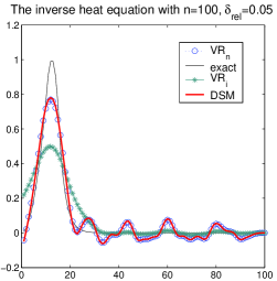
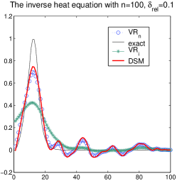
Figure 2: Plots of solutions obtained by DSM, VR for the inverse heat equation when $n=100$, $\delta_{rel}=0.05$ (left) and $\delta_{rel}=0.1$ (right).

The conclusion is that the DSM competes favorably with the VR_n in this experiment.

3.3 A linear algebraic system for the computation of the second derivatives

Let us do some numerical experiments with linear algebraic systems arising in a numerical experiment of computing the second derivative of a noisy function.

The problem is reduced to an integral equation of the first kind. A linear algebraic system is obtained by a discretization of the integral equation whose kernel $K$ is Green’s function

$$K(s,t)=\left\{\begin{matrix}s(t-1),\quad\text{if}\quad s<t\\ t(s-1),\quad\text{if}\quad s\geq t\end{matrix}\right..$$

Here $s,t\in[0,1]$ and as the right-hand side $f$ and the corresponding solution $u$ one chooses one of the following (see [4]):

$$\text{case 1},\quad f(s)=(s^{3}-s)/6,\quad u(t)=t,$$

$$\text{case 2},\quad f(s)=e^{s}+(1-e)s-1,\quad u(t)=e^{t},$$

$$\text{case 3},\quad f(s)=\left\{\begin{matrix}(4s^{3}-3s)/24,&\quad\text{if}\quad&s<\frac{1}{2}\\ (-4s^{3}+12s^{2}-9s+1)/24,&\quad\text{if}\quad&s\geq\frac{1}{2}\end{matrix}\right.,$$

$$u(t)=\left\{\begin{matrix}t,&\quad\text{if}\quad&t<\frac{1}{2}\\ 1-t,&\quad\text{if}\quad&t\geq\frac{1}{2}\\ \end{matrix}\right..$$

Using $A_{n}$ and $u_{n}$ in [4], the right-hand side $b_{n}=A_{n}u_{n}$ is computed. Again, we use $n=10,20,...,100$ and $b_{n,\delta}=b_{n}+e_{n}$, where $e_{n}$ is a vector containing random entries, normally distributed with mean 0, variance 1, and scaled so that $\|e_{n}\|=\delta_{rel}\|b_{n}\|$. This linear algebraic system is mildly ill-posed: the condition number of $A_{100}$ is $1.2158\times 10^{4}$.

Numerical results for the third case is presented in Table 5. In this case, the results obtained by the VR_n are often slightly more accurate than those of the DSM. However, the difference between accuracy as well as the difference between time of computation of these methods is small. Numerical results obtained by these two methods are much better than those of the VR_i.

Table 5: Results for the deriv2 problem with $\delta_{rel}=0.01$, $n=100$ case 3.

	DSM		VRi		VRn
$n$	$N_{\text{linsol}}$	$\frac{\|u_{\delta}-y\|_{2}}{\|y\|_{2}}$	$N_{\text{linsol}}$	$\frac{\|u_{\delta}-y\|_{2}}{\|y\|_{2}}$	$N_{\text{linsol}}$	$\frac{\|u_{\delta}-y\|_{2}}{\|y\|_{2}}$
10	4	0.0500	2	0.0542	6	0.0444
20	4	0.0584	2	0.0708	6	0.0561
30	4	0.0690	2	0.0718	6	0.0661
40	4	0.0367	1	0.0454	4	0.0384
50	3	0.0564	1	0.0565	4	0.0562
60	4	0.0426	1	0.0452	4	0.0407
70	5	0.0499	1	0.0422	5	0.0372
80	4	0.0523	1	0.0516	4	0.0498
90	4	0.0446	1	0.0493	4	0.0456
100	4	0.0399	1	0.0415	5	0.0391

For other cases, case 1 and case 2, numerical results obtained by the DSM are slightly more accurate than those by the VR_i. Figure 3 plots the numerical solutions for these cases. The computation time of the DSM in these cases is about the same as or less than that of the VR_n.

 

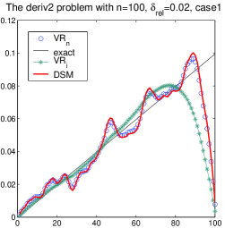
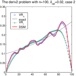
Figure 3: Plots of solutions obtained by DSM, VR for the deriv2 problem when $n=100$, $\delta_{rel}=0.02$ (left) and $\delta_{rel}=0.02$ (right).

The conclusion in this experiment is that the DSM competes favorably with the VR. Indeed, the VR_n is slightly better than the DSM in case 3 but slightly worse than the DSM in cases 1 and 2.

4 Concluding remarks

The conclusions from the above experiments are:

1. The DSM always converges for $a(t)=\frac{a_{0}}{1+t}$ given that $a_{0}>a_{op}$. However, if $a_{0}$ is not well chosen, then the convergence speed may be slow. The parameter $a_{0}$ should be chosen so that it is greater than and close to the optimal $a_{op}$, i.e., the value minimizing the quantity:

   $$\|u_{a_{op}}-y\|=\inf_{a}\|u_{a}-y\|,\quad u_{a}=T_{a}^{-1}Af_{\delta}.$$

   However, since $a_{op}$ is not known and $a_{M}$ is often close to $a_{op}$, we choose $a_{0}$ so that

   $$\delta<\|AT_{a_{0}}^{-1}A^{*}f_{\delta}-f_{\delta}\|<2\delta.$$

2. The DSM is sometimes faster than the VR. In general, the DSM is comparable with the VR_n with respect to computation time.

3. The DSM is often slightly more accurate than the VR, especially when $\delta$ is large. Starting with $a_{0}$ such that $\delta<\|AT_{a_{0}}^{-1}A^{*}f_{\delta}-f_{\delta}\|<2\delta$, the DSM often requires 4 to 7 iterations, and main cost in each iteration consists of solving the linear system $T_{a}u=A^{*}f_{\delta}$. The cost of these iterations is often about the same as the cost of using Newton’s method to solve $a_{M}$ in the VR_n.

4. For any initial $a_{0}$ such that $\delta<\|AT_{a_{0}}^{-1}A^{*}f_{\delta}-f_{\delta}\|<2\delta$, the DSM always converges to a solution which is often more accurate than that of the VR_n. However, with the same initial $a_{0}$, the VR_n does not necessarily converge. In this case, we restart the Newton scheme to solve for the regularization parameter with initial guess $a_{1}=\frac{a_{0}}{2}$ instead of $a_{0}$.

References

- [1] Burrage, K., 1995, Parallel and sequential methods for ordinary differential equations, Oxford University Press, Oxford.
- [2] Choi, M. D., 1983, Tricks or treats with the Hiblbert matrix, American Mathematical Monthly, pp. 301-312.
- [3] Hairer, E. and Nørsett, S.P. and Wanner, G., 1987, Solving ordinary differential equation I, nonstiff problems, Springer, Berlin.
- [4] Hansen, P. C., 1994, Regularization tools, A Matlab package for the analysis and solution of discrete ill-posed problems. Numerical Algorithms, pp. 1-35.
- [5] Kirsch, A., 1986, An introduction to the mathematical theory of inverse problems, Springer-Verlag, Berlin.
- [6] Ramm, A. G., 2007, Dynamical systems method for solving operator equations, Elsevier, Amsterdam.