SNO+: predictions from standard solar models and resonant spin flavour precession

Marco Picariello${}^{a\,b}$ , João Pulido^a
a Centro de Física Teórica das Partículas (CFTP)
Departamento de Física, Instituto Superior Técnico
Av. Rovisco Pais, P-1049-001 Lisboa, Portugal
^b I.N.F.N. - Lecce, and Dipartimento di Fisica
Università di Lecce
Via Arnesano, ex Collegio Fiorini, I-73100 Lecce, Italia
S. Andringa, N.F. Barros, J. Maneira
Laboratório de Instrumentação e Física Experimental de Partículas,
Av. Elias Garcia, 14, 1^∘, 1000-149 Lisboa, Portugal

Time variability of the solar neutrino flux especially in the low and intermediate energy sector remains an open question and, if it exists, it is likely to be originated from the magnetic moment transition from active to light sterile neutrinos at times of intense solar activity and magnetic field. We examine the prospects for the SNO+ experiment to address this important issue and to distinguish between the two classes of solar models which are currently identified as corresponding to a high (SSM I) and a low (SSM II) heavy element abundance. We also evaluate the predictions from these two models for the Chlorine experiment event rate in the standard LMA and LMA+Resonant Spin Flavour Precession (RSFP) scenarios. It is found that after three years of SNO+ data taking, the pep flux measurement will be able to discriminate between the standard LMA and LMA+RSFP scenarios, independently of which is the correct solar model. If the LMA rate is measured, RSFP with $B_{0}\sim 280kG$ for the resonant $\Delta m^{2}_{01}$ can be excluded at more than $4\sigma$. A low rate would signal new physics, excluding all the 90$\%$ allowed range of the standard LMA solution at 3$\sigma$, and a time variability would be a strong signature of the RSFP model. The CNO fluxes are the ones for which the two SSM predictions exhibit the largest differences, so their measurement at SNO+ will be important to favour one or the other. The distinction will be clearer after LMA or RSFP are confirmed with pep, but still, a CNO measurement at the level of SSM I/LMA will disfavour SSM II at about $3\,\sigma$. We conclude that consistency between future pep and CNO flux measurements at SNO+ and Chlorine would either favour an LMA+RSFP scenario or favour SSM II over SSM I.

1 Introduction

Neutrino oscillations in matter [1] with the resonant amplification of a small vacuum mixing angle [2], although a much attractive mechanism, has not proven to be the origin of the solar neutrino deficit. While also an oscillation and resonant effect, the large mixing angle solution (LMA) [3, 4, 5] has instead become generally accepted as the dominant one [6, 7, 8]. In the LMA mechanism the conversion from active electron neutrinos produced in the solar core to weakly interacting ones of another flavour takes place through a strongly adiabatic resonance occuring still at the solar core. The order parameter is a large vacuum mixing of the order of $30^{o}-33^{o}$.

On the other hand, the time variability of the active neutrino event rate had been hinted long ago by the Chlorine collaboration [9] who suggested a possible anticorrelation of active neutrino flux with sunspot activity. It was then interpreted by Voloshin, Vysotskii and Okun [10] as a neutrino magnetic moment effect, such that an intense sunspot activity would induce a conversion of a large fraction of neutrinos into undetectable ones (either steriles or of a different flavour) through the interaction of the magnetic moment with the solar magnetic field. Hence a more intense solar activity would correspond to a smaller flux of detectable neutrinos and viceversa. An interesting evolution of this proposal was the suggestion in 1987 by Lim and Marciano [11] and by Akhmedov [12] that the neutrino spin flavour precession could take place anywhere inside the sun via a resonant process. This enhances the mechanism and allows for a smaller neutrino magnetic moment in order to produce a visible effect. The resonant spin flavour precession (RSFP) bears a resemblance to matter oscillations and is a result of the balance between matter density and the product $\mu_{\nu}B$ (neutrino magnetic moment times the solar field).

The interpretation of solar data is at present still partly ambiguous, with several scenarios involving RSFP [13, 14] and non-standard neutrino interactions [15] being viable. Our knowledge of the solar neutrinos relies essentially on the data from the high energy sector (mainly the ${}^{8}B$ flux), whereas the overwhelming low and intermediate energy one remains vastly unknown, except for the integrated measurements provided by the radiochemical experiments. As pointed out earlier [16], the observed decrease of the Gallium event rate [17] opens the question of whether there is time variability affecting only the low energy sector and has motivated the investigation of RSFP to light sterile neutrinos in combination with LMA . LMA+RSFP thus requires a sizable neutrino magnetic moment and a strong field at times of intense solar activity and a weak field otherwise, which causes the modulations in the neutrino event rate. Low energy solar neutrino experiments like Borexino [18, 19], KamLAND [6, 7] and SNO+ will no doubt help in clarifying the situation within the next few years. The first Borexino data, very recently released [19], are compatible with the RSFP model predictions [13, 16] earlier derived since those data were taken during the present year (2007) when the magnetic solar activity is at a minimum.

Besides our limited knowledge of the low energy neutrino sector, one of the key inputs of solar models, namely the amount of heavy element abundance relative to hydrogen, $Z/X$, is still unclear [20]. This affects the neutrino fluxes, in particular most strongly the CNO ones and to a lesser extent the ${}^{7}Be$ one. Two classes of standard solar models (SSMs) may at present be distinguished [21, 22], one with a ’high’ value of $Z/X$ [23] and another with a ’low’ one [24], hereby denoted by SSM I and SSM II, respectively. In the first the metallicity is consistent with sound speed, convective zone depth and density profiles, in excellent agreement with helioseismology. Such is not the case in the second one which is however based on an improved modeling of the solar atmosphere. As uncertainties are considerable, we will in the present paper take both models into account .

The purpose of this paper is to analyse the possibility of the proposed SNO+ experiment to ascertain on whether RSFP occurs at low and/or intermediate energies. We will also investigate the possible signatures of the two classes of SSMs, in particular whether it is possible to distinguish between them with data from the forthcoming SNO+ and from the Chlorine [25] experiment. For neutrino-electron scattering experiments, sensitivity to neutrino physics depends on the accuracy of solar models, since the calculation of the electron neutrino survival probability relies on the comparison of the measured flux with the total predicted flux. So for the purpose of distinguishing models with different survival probabilities, the best sensitivity lies in the observation of the solar flux component with the smallest error. Above the threshold of liquid scintillator electron scattering experiments, the component with the most accurate prediction is the monoenergetic (1.442 MeV) source of pep neutrinos. The pep flux also has the smallest spread in the predictions from the main solar models, which allows its measurement to be sensitive to Neutrino physics without needing to choose a particular solar model.

The paper is divided as follows: in Section 2 we briefly review the RSFP model and its motivations, and compare its predictions with standard LMA for the existing Chlorine experiment data, in the context of the two SSMs. In Section 3 we briefly describe the SNO+ experiment. In Sec. 4.1 we describe the method and present our results. In Section 4.2 we comment on the sensitivity of the pep measurement to an RSFP effect and we investigate the possibility for SNO+ to distinguish between SSMs of the two types with the CNO measurement in Sec. 4.3. Finally in Section 5 we report our conclusions.

2 Resonant spin flavour precession and solar models

In this Section we describe the RSFP effect from active to light sterile neutrinos and evaluate the survival probability for LMA and LMA+RSFP (non-vanishing $\mu_{\nu}$ with low and high solar magnetic field). We start with a brief review of the model presented in ref. [16] whose predictions for Borexino and LENS were analyzed in [13] and for KamLAND in [26]. We also evaluate the event rates in the Chlorine experiment for standard neutrinos (i.e. massless and with no magnetic moment), for the LMA and LMA+RSFP scenario and for standard LMA (vanishing $\mu_{\nu}$). We use the neutrino fluxes from the type I [23] and II [24] solar models.

2.1 Resonant Spin Flavour Precession

The possible anticorrelation with sunspot activity of the electron neutrino flux in the Ga experiments is most naturally explained in terms of a resonant conversion to neutrinos of other types that are unseen by the weak charged current. As shall be discussed, this requires a mass square difference between the intervening neutrino flavours in the resonance $\Delta m^{2}_{01}=O(10^{-8}eV^{2})$. Such a value implies that conversion to weakly interacting neutrinos is excluded, leaving us the possibility of conversion to sterile neutrinos. The simplest departure from conventional LMA able to generate such a conversion is provided by a model which, in addition to the two flavours involved in LMA, introduces a sterile neutrino with a vanishing vacuum mixing. The active states $\nu_{e},\nu_{\mu}$ communicate to the sterile one via a single magnetic moment. Owing to the large order of magnitude difference between the parameters $\Delta m^{2}_{21}$ and $\Delta m^{2}_{01}$ (associated with the LMA and SFP resonances respectively) the two resonances are located far apart, so that they do not interfere. A straightforward but long calculation leads to the following form of the Hamiltonian [16]

$$\cal{H}_{\rm{M}}=\left(\begin{array}[]{ccc}\frac{-\Delta m^{2}_{10}}{2E}&\mu_{\nu}B&0\\ \mu_{\nu}B&\frac{\Delta m^{2}_{21}}{2E}s^{2}_{\theta}+V_{e}&\frac{\Delta m^{2}_{21}}{4E}s_{2\theta}\\ 0&\frac{\Delta m^{2}_{21}}{4E}s_{2\theta}&\frac{\Delta m^{2}_{21}}{2E}c^{2}_{\theta}+V_{\mu}\end{array}\right)$$ (1)

in the mass matter basis $(\tilde{\nu}_{0}~{}\tilde{\nu}_{1}~{}\tilde{\nu}_{2})$. In this equation $V_{e}$, $V_{x}$ are the matter induced potentials for $\nu_{e}$ and $\nu_{x}$, $B$ is the solar magnetic field and $\theta$ is the vacuum mixing angle.

The important transition with order parameter $\mu_{\nu}B$ and whose time dependent efficiency may determine the possible modulation of neutrino flux is therefore between mass matter eigenstates $\tilde{\nu}_{0}$, $\tilde{\nu}_{1}$. It is expected to resonate in the region where the magnetic field is the strongest in the period of high solar activity. We consider the Landau Zener approximation in dealing with the two resonances. Since the LMA one is strongly adiabatic, we need only to consider the jump probability between $\tilde{\nu}_{0}$, $\tilde{\nu}_{1}$ in the vicinity of the SFP resonance .

In the LMA+RSFP scenario active neutrinos are partially converted to light sterile ones at times of strong solar magnetic field, thus leading to the lower Gallium event rate in the period 1998-2003 [17], while LMA acts alone otherwise and the higher rate is obtained. As in previous publications, throughout our RSFP calculations we use a value for the neutrino magnetic moment $\mu_{\nu}=10^{-12}\mu_{B}$. For a definite neutrino energy the critical density is fixed by the order of magnitude of the corresponding mass squared difference and determines the resonance range. Furthermore it has been noticed [27] that the solar rotation frequency matches the observed neutrino modulation in the equatorial section of the convection zone near the tachocline, at $\simeq(0.7-0.8)R_{S}$. This indicates a field profile whose time dependent peak occurs around this depth. In order that the low and intermediate energy neutrino SFP resonance is located in this range, so as to provide time modulation in this sector, one needs $\Delta m^{2}_{01}=O(10^{-8})eV^{2}$. Hence, owing to the absence of interference between the two resonances (LMA and RSFP) the high energy solar neutrino experiments (SuperKamiokande [28] and SNO [8]) are not expected to exhibit any time modulation in their event rate. On the contrary, of all the experiments so far, Gallium will be the most sensitive of all to variability, while Chlorine may lie in the borderline with some moderate variability which failed to be clearly detected.

Based on the above criteria we chose solar field profiles as in fig.1 of ref. [13]. In our previous publications [16, 13, 30] we performed two separate fits for the high and low Gallium event rates together with all other solar neutrino data. We also investigated the dependence of the results on the choice of solar field profile and on the value of $\Delta m^{2}_{01}$. We will in the present paper use our best choices from ref. [30], namely

$$B=\frac{B_{0}}{cosh[6(x-x_{c})]}~{}~{}~{}0<x<x_{c}$$ (2)

$$B=\frac{B_{0}}{cosh[15(x-x_{c})]}~{}~{}~{}x_{c}<x<1$$ (3)

for the field profile and

$$\Delta m^{2}_{01}=-1.7\times 10^{-8}eV^{2}.$$

Here $B_{0}$ is the peak field value, which for active sun we take to be $280kG$, $x$ is the fraction of the solar radius and $x_{c}=0.71$.

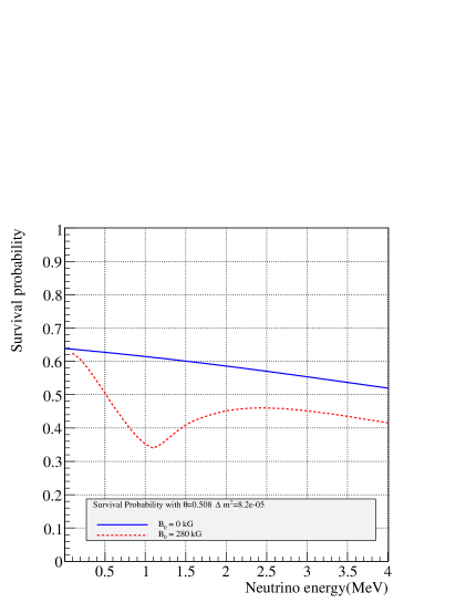
Figure 1: Electron neutrino survival probability for LMA (zero field) and LMA+RSFP for the considered point. For the RSFP case we use a peak field value $B_{0}=280kG$ and a profile as in [29, 30].

Furthermore we use [29, 30]

$$\theta=0.508,~{}~{}\Delta m^{2}=8.2\times 10^{-5}eV^{2}$$ (4)

which lie within $1\sigma$ of the central values for KamLAND[7]. The field profile chosen, together with the value of $\Delta m^{2}_{01}$, will be responsible for a modulation shared by $pp$ and ${}^{7}Be$ neutrinos and a dip at the low and intermediate energy in the survival probability. This is shown in fig.1.

2.2 Chlorine rate, type I and II solar models

	$\phi_{j}(cm^{-2}s^{-1})$		$R_{j}$ (SNU)
	SSM I	SSM II	SSM I	SSM II
pep	$1.42\times 10^{8}(1\pm 0.015)$	$1.45\times 10^{8}(1\pm 0.01)$	0.222 $\pm$0.003	0.226 $\pm$0.002
${}^{7}Be$	$4.84\times 10^{9}(1\pm 0.105)$	$4.34\times 10^{9}(1\pm 0.093)$	1.16 $\pm$0.122	1.043 $\pm$0.097
${}^{8}B$	$5.69\times 10^{6}(1\pm 0.16)$	$4.51\times 10^{6}(1\pm 0.12)$	6.740 $\pm$1.078	5.342 $\pm$0.641
${}^{13}N$	$3.05\times 10^{8}(1\pm^{0.31}_{0.28})$	$2.00\times 10^{8}(1\pm^{0.145}_{0.127})$	0.052 $\pm^{0.016}_{0.014}$	0.034 $\pm^{0.005}_{0.004}$
${}^{15}O$	$2.31\times 10^{8}(1\pm^{0.33}_{0.29})$	$1.44\times 10^{8}(1\pm^{0.165}_{0.142})$	0.154 $\pm^{0.051}_{0.045}$	0.096 $\pm^{0.016}_{0.014}$
$\Sigma R_{Cl}$			$8.33\pm 1.2$1	$6.74\pm 0.73$

Table 1: Predicted total fluxes ($\phi_{j}$) and expected event rates ($R_{j}$) in the Chlorine experiment for standard neutrinos.

Here we analyse the Chlorine event rates in the two scenarios, the one with and the one without neutrino magnetic moment, using the neutrino fluxes from SSM I [23] and SSM II [24]. It will be seen, from the comparison of these predictions with the Chlorine data [25]

$$R_{Cl}=2.56\pm 0.16\pm 0.15~{}SNU,$$ (5)

that RSFP is compatible with both solar models while standard LMA favours SSM II. The predicted fluxes $\phi_{j}$, the partial event rates $R_{j}$ for each flux and the total event rate for the Chlorine experiment $R_{Cl}$ are given in table (1) for both models with standard neutrinos. The errors in the partial event rates $\delta R_{j}$ listed in this table were calculated from

$$R_{j}=\int\,\sigma{{}_{{}_{Cl}}}\,\phi{{}_{{}_{j}}}\left(1\pm\frac{\delta\phi_{j}}{\phi_{j}}\right)dE_{\nu}=\bar{R}_{j}\pm\delta R_{j}$$ (6)

for flux $j$ that is, only the flux errors were considered.

	$R_{LMA}$ (SNU)		$R_{RSFP}$ (SNU)
	SSM I	SSM II	SSM I	SSM II
pep	0.133 $\pm$0.002	0.136 $\pm$0.001	0.088 $\pm$0.001	0.090 $\pm$0.001
${}^{7}Be$	0.710 $\pm$0.075	0.637 $\pm$0.059	0.447 $\pm$0.047	0.401 $\pm$0.037
${}^{8}B$	2.003 $\pm$0.320	1.587 $\pm$0.191	1.888 $\pm$0.302	1.497 $\pm$0.180
${}^{13}N$	0.032 $\pm^{0.010}_{0.009}$	0.021 $\pm{0.003}$	0.019 $\pm^{0.006}_{0.005}$	0.012 $\pm{0.002}$
${}^{15}O$	0.091 $\pm^{0.030}_{0.026}$	0.057 $\pm^{0.009}_{0.008}$	0.059 $\pm^{0.019}_{0.017}$	0.037 $\pm^{0.006}_{0.005}$
$\Sigma R_{Cl}$	2.97$\pm$0.40	2.44$\pm$0.25	2.50$\pm$0.35	2.04$\pm$0.22

Table 2: Expected event rates in the Chlorine experiment for the two SSMs. For the parameter choices used in the LMA and LMA+RSFP cases, see the main text [eq. (4)] and fig. 1.

The results for the event rates are given in table (2) for LMA with parameters as in eq. (4) and LMA+RSFP. The errors in the total Chlorine rate are obtained using the correlation among the flux errors as in tables 16 and 17 of ref. [21]. Comparing the event rates for LMA (zero field) and LMA + RSFP (high field), it is seen that some modulation is expected in both SSMs, due to the time dependence of the solar magnetic field.

Averaging the results

$$SSM~{}I~{}~{}~{}~{}\bar{R}_{Cl}=2.73\pm 0.38SNU,$$ (7)

$$SSM~{}II~{}~{}~{}~{}\bar{R}_{Cl}=2.24\pm 0.23SNU$$ (8)

we see that both SSMs are fully compatible with the data. That is not the case when using for $\theta_{12},~{}\Delta m^{2}_{21}$ the central values of standard LMA, that correspond to a negligible magnetic moment, from global solar analysis and KamLAND [8, 31]:

$$\theta=0.592,~{}~{}\Delta m^{2}=8.0\times 10^{-5}eV^{2}.$$ (9)

In fact, in this case the Chlorine rate is fully compatible with the SSM II model while SSM I is slightly disfavoured at 1.3$\sigma$. The predictions obtained from the solar neutrino and KamLAND global analysis central values are shown in Table (3).

	$R$ (SNU)
	SSM I	SSM II
pep	0.120 $\pm 0.002$	0.123 $\pm 0.001$
${}^{7}Be$	0.638 $\pm 0.067$	0.572 $\pm 0.053$
${}^{8}B$	2.351 $\pm 0.376$	1.864 $\pm 0.224$
${}^{13}N$	0.028 $\pm^{0.009}_{0.008}$	0.019 $\pm^{0.003}_{0.008}$
${}^{15}O$	0.082 $\pm^{0.027}_{0.024}$	0.051 $\pm^{0.002}_{0.007}$
$\sum R_{Cl}$	3.22 $\pm 0.45$	2.63 $\pm 0.27$

Table 3: Expected event rates in Chlorine for standard LMA with Solar+KamLAND bestfit parameters: $\theta=0.592$, $\Delta m^{2}=8.0\times 10^{-5}$.

3 The SNO+ experiment

Among the existing and proposed solar neutrino experiments to come online in the near future, SNO+ will be the only one with the ability to measure a survival probability, as the ratio between the measured and SSM predicted rate of a solar neutrino component, at the precision level of 5%. Due to the depth of SNOLAB, SNO+ will have a low level of ${}^{11}C$ background, allowing for an accurate measurement of the the pep neutrino flux - predicted in the SSM with an error of (1-1.5)%. This is an advantage over the measurement of the ${}^{7}Be$ flux, that can be done earlier in other experiments (Borexino, KamLAND), but is predicted with an error of (9.3-10.5)%. In addition, SNO+ will also be the best experiment to measure the CNO-cycle fluxes. Measurements of the pep and CNO fluxes will be possible also in Borexino[38], although with larger systematic and statistical uncertainties than at SNO+. The expected accuracy on these fluxes will allow for the distinction between different Solar Models accepted by the present data. In addition, SNO+ will measure reactor anti-neutrinos, geo-neutrinos and can later be upgraded to detect neutrinoless double-beta decays, in order to search for the absolute neutrino mass.

3.1 The SNO+ detector

SNO+ [32, 33] is a proposed upgrade of the the Sudbury Neutrino Observatory (SNO) detector [34], in which the heavy water target will be replaced by an organic liquid scintillator. The scintillator was chosen to have a good light yield and transparency, and to be compatible with the existing SNO components: chemical and optical compatibility with the acrylic vessel and emission wavelength peaks close to the PMT response.

SNO+ has a fiducial volume of  1000 tonnes, in a 12m diameter acrylic vessel viewed by 9456 PMTs mounted on an 18 m diameter geodesic structure. The PMTs have a diameter of 20 cm, and are coupled to optical reflectors, increasing the total effective coverage to 54%. The region outside the acrylic vessel is filled with 7000 tonnes of light water (1700 tonnes within the PMT structure), acting as a shield against external radiation. The external regions viewed by additional 114 PMTs, to act as a veto for cosmic ray muons.

The large volume of the detector will allow for an effective veto of external backgrounds (mainly gammas and neutrons) through position reconstruction, while maintaining a large fiducial volume. Concerning internal radioactivity, the purity levels achievable for scintillators can be estimated from the existing KamLAND ones for the U and Th chains, while others such as ${}^{40}K$ and ${}^{210}Bi$ are being studied for several experiments and expected to be reduced by several orders of magnitude.

In addition, the center of the SNO detector is at a depth of 2092m, or 6010 m of water equivalent - it is located in the deepest underground physics facility, SNOLAB. The ${}^{11}C$ contamination produced by cosmic ray muons - which in general prevents or severely hinders the measurement of the pep solar neutrino line - is not a problem at SNO+ since at this depth there are only approximately 70 muons to enter the detector per day, and so the data taken just after can be cut away.

The fact that SNO+ is located in a laboratory whose background conditions are well known and has the same geometry as the SNO detector, allows for accurate estimations of its capabilities even before construction.

3.2 Neutrino Measurements at SNO+

Neutrinos interact in the scintillator through elastic scattering off electrons ($\nu e^{-}\to\nu e^{-}$). In the energy range of pep solar neutrinos, the cross-section is around five times smaller for muon or tau neutrinos than for electron neutrinos, so SNO+ is primarily a ”disappearance experiment” for electron neutrinos, even if there is some sensitivity to the other flavors of active neutrinos.

The high light yield of the scintillator - about 100 times more light than the Cerenkov light in heavy water - allows the detection of recoil electrons with energies as low as tens of keV.

Since the measured energy will be roughly proportional to the number of detected scintillation photons, the main contribution to the energy resolution can be written as:

$$\frac{\sigma(E)}{E}=\frac{1}{\sqrt{N_{ph}}}\times\frac{1}{\sqrt{E}}$$ (10)

where $N_{ph}$ is the detected light yield which, from conservative Monte Carlo simulations [35], was estimated at about $N_{ph}=600$ photons per MeV. This results in an energy resolution of 4% at 1 MeV, better than in other large liquid scintillator detectors – 6.2% at KamLAND[7] and 5% at Borexino[36].

The energy of the incoming neutrino is not directly reconstructed, but the different electron spectra structures - and mainly the Compton edge directly related to the neutrino energy - can be used to statistically separate the neutrino signal from background and the different contributions to the solar neutrino flux, namely the mono-energetic pep line.

The high rate low energy background from ${}^{14}C$ in the scintillator and the gamma background from detector materials can be suppressed with data selection cuts in both energy – threshold of 500 keV – and position. For the pep analysis, an energy window from 800 keV to 1500 keV is expected, to avoid background from fluctuations of the ${}^{7}Be$ signal on the lower side.

Assuming U and Th background levels from KamLAND and the expected levels for ${}^{40}K$ and ${}^{210}Bi$ after purification, SSM shapes for CNO neutrinos and LMA oscillation, a likelihood fit to the energy spectrum allows the separate measurement of the number of pep (CNO) neutrino events with a 4% (6%) uncertainty[35], after three years of data taking. Adding in a global systematic uncertainty on the fiducial volume, estimated at 3%, a total flux measurement error of 5% is obtained for pep.

4 Sensitivity of SNO+ to RSFP and solar models

In this section we calculate the predicted event rates of pep and CNO solar neutrinos in SNO+ for the LMA+RSFP model in the high and low field cases, for the two sets of solar models, SSM I and SSM II (Sec. 4.1). We then use the predicted rates to estimate how sensitive is SNO+ to an RSFP effect (Section 4.2), and to the discrimination between the two solar models, SSM I and SSM II (Section 4.3).

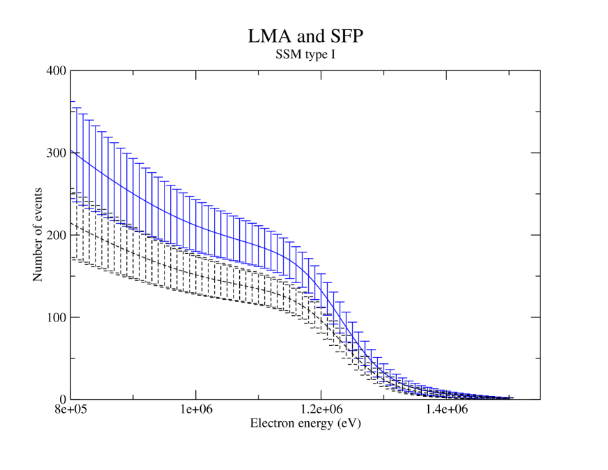
Figure 2: Standard LMA and LMA+RSFP spectra in the active sun period for type I model (SSM I [23]).

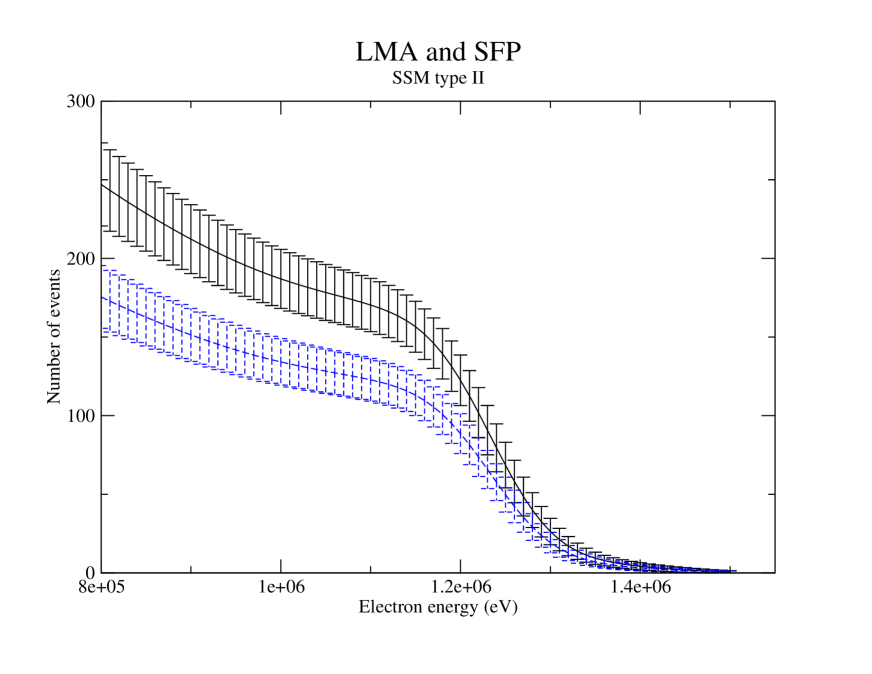
Figure 3: Same as fig.3 for type II model (SSM II [24]).

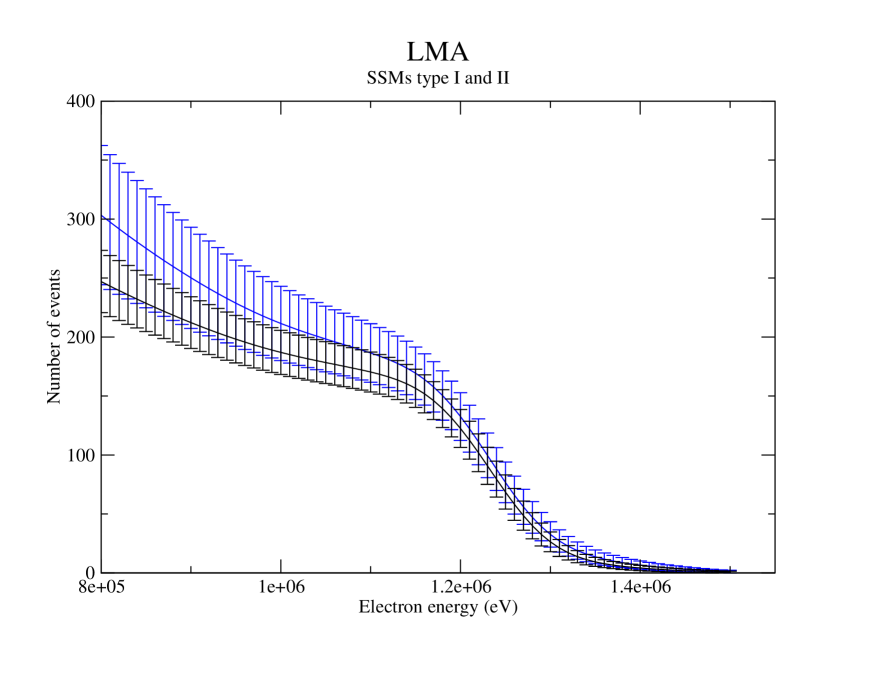
Figure 4: Standard LMA spectrum for models of type I (SSM I [23]) and type II (SSM II [24]).

4.1 Expected rates and spectral analysis

The expected event rate for each solar neutrino component can be given by

$$R(j) = V_{fid}\,\rho_{e}\,\int_{T_{min}}^{T_{max}}dT_{m}\int_{0}^{\infty}dT\,F(T,T_{m})\int_{0}^{E_{max}}dE\,\phi_{j}\Phi_{j}(E)\,P_{\nu_{x}}(E)\,\frac{d\sigma_{\nu_{x}}(E,T)}{dT}.$$ (11)

The total fluxes $\phi_{j}$ for each component $j\in\{pep,N,O\}$ are taken from table (1). $\Phi_{j}(E)$ is the normalized neutrino flux spectrum for flux $j$ (delta function for pep). Eq. (11) includes a sum over $x\in\{e,\mu,\tau\}$. The quantity $T_{m}$ is the observed electron kinetic energy, $T$ is the true electron kinetic energy, $E$ is the neutrino energy with $E_{max}$ given by the kinematics and $T_{min}$, $T_{max}$ are the lower and upper thresholds of the $T_{m}$ analysis energy window, given in Section 3. $\rho_{e}$ is the electron density of the scintillator and $V_{fid}$ is the analysis fiducial volume. $P_{\nu_{x}}(E)$ is the probability for $\nu_{e}$ $\rightarrow$ $\nu_{x}$ conversion, $d\sigma_{\nu_{x}}(E,T)/dT$ is the cross section for $\nu_{x}e$ scattering and $F(T,T_{m})$ is the response function of the detector. This is given by

$$F(T,T_{m}) = \frac{1}{\sigma\sqrt{2\pi}}\exp\left(-\frac{(T-T_{m})^{2}}{2\sigma^{2}}\right)$$ (12)

where $\sigma$ is the detector energy resolution, as described by Eq. 10. For models I and II we compute the contribution from each component of the solar neutrino spectrum: $pep$, ${}^{15}O$, and ${}^{13}N$ (the ${}^{17}F$ contribution is negligible and is not evaluated).

We perform the rate calculation for four scenarios:

SFP

The oscillation probabilities $P_{\nu_{x}}$ are computed with the RSFP effect in addition to LMA as explained in Section 2.1 and in [13, 16]. We consider a high field value of $B_{0}=280kG$, which would correspond to the first three years of data taking, since SNO+ is expected to start during the next period of rising solar activity including its maximum around 2011[37].

SFP0

$P_{\nu_{x}}$ are obtained from the LMA oscillation effects with $\Delta m^{2},~{}\theta$ as in eq. (4), corresponding to $B_{0}=0kG$, the RSFP prediction for low solar activity periods.

LMA

$P_{\nu_{x}}$ are obtained from the LMA oscillation effects with Solar+KamLAND bestfit $\Delta m^{2},~{}\theta$, as in eq. (9).

NOsc

For reference we also evaluated the case for the absence of oscillations, where $P_{\nu_{x}}=\delta_{x,e}$ .

The extraction of the pep and CNO signals from the future experimental data will be based on a fit to the measured energy spectrum, which will require a very accurate knowledge of the detector response, as well as of the residual backgrounds that pass the selection cuts, based on extensive detector calibrations. The SNO+ collaboration has carried Monte Carlo simulations [35] of the expected backgrounds in the pep-CNO energy window, and performed maximum likelihood signal extraction on the simulated signals and backgrounds, mostly from isotopes of the ${}^{238}U$ and ${}^{232}Th$, as well as ${}^{40}K$. The resulting sensitivity strongly depends on the background levels. Assuming the target values for KamLAND, a sensitivity of 4% for pep and 6% for CNO is obtained for three years of data.

This calculation assumed standard LMA oscillations, and might be changed in the case of RSFP, in which the signals are reduced. We carry out a simple spectral analysis, without considering the backgrounds, for all cases.

The energy spectrum, or expected number of events in the spectral bin i is given by:

$$N_{i} = \epsilon\,\int_{T_{i}}^{T_{i+1}}dT_{m}\int_{0}^{\infty}dT\,F(T,T_{m})\int_{0}^{E_{max}}dE\,\phi_{j}\Phi_{j}(E)\,P_{\nu_{x}}(E)\,\frac{d\sigma_{\nu_{x}}(E,T)}{dT}$$ (13)

where $\epsilon=Livetime\times V_{fid}\rho_{e}\,$ is the exposure, and the sum extends over the flux index $j\in\{pep,N,O\}$.

The contributions to uncertainty ($\delta N_{i}$) include:

• the statistical error, considering the number of events N for 3 years;

• the energy scale error (we assumed an error of $10keV$ in the determination of the threshold);

• a global systematic error of 3% from the fiducial volume determination;

• the error in the total flux predictions as given in table (1).

The error for each bin is obtained by adding quadratically these four sources of error:

$$\delta N_{i} = \sqrt{\Big{(}\sqrt{N_{i}}\Big{)}^{2}+\Big{(}\delta N_{i}^{\mbox{scale}}\Big{)}^{2}+\Big{(}N_{i}*3\%\Big{)}^{2}+\Big{(}\delta N_{i}^{\mbox{flux}}\Big{)}^{2}},$$ (14)

where the first three terms are experimental errors (statistical, energy scale, and global systematic uncertainty) and the last is the theoretical one (flux uncertainty). Our extraction uncertainties are in reasonable agreement with the values quoted in [35], before including the theoretical and energy scale errors, and can thus be taken as indicative values. As expected, the CNO extraction uncertainty is increased in the RSFP case, and that is taken into account by this procedure. Equation 13 can be rewritten in matrix form as:

$$N_{i}=F_{ij}\;\phi_{j}.$$ (15)

Here the normalized predicted spectra of each component $F_{ij}$ is a $100\times 3$ matrix. Once the data on $N_{i}$ are known, one can extract $\phi_{j}$ by inverting F:

$$\phi_{j}=F^{-1}_{ji}\;N_{i}$$ (16)

where the $3\times 100$ matrix $F^{-1}=\left(F^{T}\;F\right)^{-1}\;F^{T}$ is the pseudoinverse of $F$ and the transpose of $F$, $F^{T}$, is a $3\times 100$ matrix. The errors are also calculated from this matrix inversion, assuming full correlation (uncorrelation) between the systematic (statistic) errors in each bin.

The spectra used in this analysis are shown in Figures 2-4. The rate results for type I and II models are shown in Tables (4) and (5).

	Number of events (in thousands) from SSM I
Component	RSFP	RSFP0	LMA	NOsc
pep	$4.82\pm 0.28$	$6.55\pm 0.38$	$6.09\pm 0.36$	$9.98\pm 0.58$
	$(\pm 0.11)$	$(\pm 0.15)$	$(\pm 0.14)$	$(\pm 0.23)$
${}^{13}N$	$0.26\pm 0.09$	$0.40\pm 0.14$	$0.38\pm 0.13$	$0.60\pm 0.21$
	$(\pm 0.03)$	$(\pm 0.05)$	$(\pm 0.05)$	$(\pm 0.07)$
${}^{15}O$	$2.61\pm 0.86$	$3.63\pm 1.20$	$3.38\pm 1.11$	$5.52\pm 1.82$
	$(\pm 0.09)$	$(\pm 0.13)$	$(\pm 0.12)$	$(\pm 0.20)$
Total	$7.69\pm 1.04$	$10.58\pm 1.45$	$9.85\pm 1.35$	$16.09\pm 2.20$
	$(\pm 0.23)$	$(\pm 0.33)$	$(\pm 0.31)$	$(\pm 0.50)$

Table 4: Expected number of events in 3 years of SNO+ from $pep$, ${}^{15}O$ and ${}^{13}N$ solar neutrinos for three years of data taking, assuming the type I model, considering LMA+RSFP, at high field (RSFP) and at low field (RSFP0), standard LMA and the no oscillation case. The error in parentheses is from the energy scale uncertainty only. The total error is indicated next to the predicted value and includes also the uncertainties from the model, from statistics and systematics, as stated in the text.

	Number of events (in thousands) from SSM II
Component	RSFP	RSFP0	LMA	NOsc
pep	$4.92\pm 0.29$	$6.68\pm 0.38$	$6.22\pm 0.36$	$10.19\pm 0.58$
	$(\pm 0.11)$	$(\pm 0.16)$	$(\pm 0.15)$	$(\pm 0.24)$
${}^{13}N$	$0.17\pm 0.03$	$0.26\pm 0.05$	$0.25\pm 0.05$	$0.39\pm 0.08$
	$(\pm 0.02)$	$(\pm 0.03)$	$(\pm 0.03)$	$(\pm 0.05)$
${}^{15}O$	$1.63\pm 0.27$	$2.26\pm 0.38$	$2.11\pm 0.35$	$3.44\pm 0.57$
	$(\pm 0.06)$	$(\pm 0.08)$	$(\pm 0.08)$	$(\pm 0.12)$
Total	$6.72\pm 0.48$	$9.25\pm 0.67$	$8.58\pm 0.62$	$14.02\pm 1.01$
	$(\pm 0.19)$	$(\pm 0.27)$	$(\pm 0.25)$	$(\pm 0.41)$

Table 5: Same as Table 4 for SSM II.

4.2 Analysis of the pep results

The most relevant aspect of the pep results is the large difference between the LMA and RSFP predictions, that is not significantly affected by our present uncertainty on the solar model.

In fact, even if the the lowest central value for the best-fit LMA prediction (in SSM I) is measured, it is high enough to exclude the highest RSFP value (in SSM II), at more than 4$\sigma$, and if it would be down by 1$\sigma$ of the prediction, RSFP would still be disfavoured at around 3$\sigma$.

On the other hand, if SNO+ finds a pep flux lower than $1.40\times 10^{8}\,cm^{-2}s^{-1}$, it will necessarily follow that new physics is at work. If the RSFP effect is observed, and the central value predicted in SSM II for $B_{0}=280kG$ is measured, the best fit LMA point is excluded at 3.3$\sigma$. In this case, all the allowed $90\%$ C.L. region of LMA is also excluded at the 3$\sigma$ level.

In addition to a low pep measurement, RSFP predicts significant time variations of the measured flux with a solar cycle periodicity, due to the dependence of the survival probability on the magnetic field peak. This expected variation would allow the distinction between RSFP and other scenarios that predict lower rates regardless of the magnetic field.

The effect is shown for field values different from $B_{0}=280kG$ in figure 5, for $\Delta m^{2}_{01}$ values around the resonant value obtained from [29, 30]. We plot in fig 5 the expected rate reduction for the $pep$ flux in relation to the non-oscillation case as a function of the solar magnetic field and $\Delta m^{2}_{01}$. From tables (4) and (5) it is readily seen that $B_{0}=0$ (the x-axis in fig 5) corresponds to a rate reduction of $65\%$.

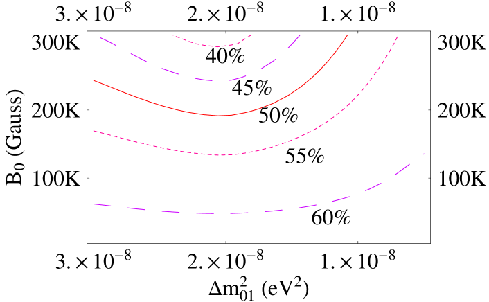
Figure 5: The expected rate reduction for the $pep$ flux with respect to the non-oscillation case, as a function of the peak value $B_{0}$ of the solar magnetic field and $\Delta m^{2}_{01}$.

4.3 Analysis of the CNO results

RSFP would change also the CNO rates in a consistent way, and that could serve as an independent cross-check of the oscillation model. However, the prediction for CNO rates depends strongly on the SSM considered and has a large uncertainty within SSM I.

In fact examining, for example, the ${}^{15}O$ contribution in the LMA case and taking into account both the theoretical and experimental errors, we see that model I predicts $3383\pm 1047$ events, while model II predicts of $2109\pm 361$ events, so that the two results overlap only slightly. This is also the case for the RSFP predictions, so that after the oscillation pattern is established with pep, the distinction between SSMs is improved.

If the central values of SSM I would be measured, SSM II could be excluded at around 2.6$\sigma$, both in LMA and RSFP cases. The $1\sigma$ upper edge of the prediction would allow a full exclusion at more than $4.6\sigma$, while the lower edge is compatible with SSM II. The large uncertainty in SSM I makes is harder to exclude, even if the measurements are in full agreement with SSM II predictions. The results could, in turn, be used to constrain the upper values of CNO fluxes allowed in this model.

We see that SNO+ will be able to determine the ${}^{13}N$ and ${}^{15}O$ fluxes with such a precision that it can discriminate SSM of type I from SSM of type II, or severely constrain SSM I. There is no doubt that the discrimination of the several flux components with this precision will have an impact on our present knowledge of the solar models. However, an answer to the question How well SNO+ discriminates SSM I from SSM II can be obtained only after the experimental data are available.

4.4 SNO+, Borexino and KamLAND

We conclude this section with a brief comparison of the model predictions for these three real time liquid scintillator experiments. We used the parameter values considered before ($\Delta m^{2}_{10}=1.7\times 10^{-8}eV^{2}$, $B_{0}=280kG$), the field profile as in eqs. (2), (3) and $\Delta m^{2}_{21}$, $\theta$ as in eq.(4). The results for the ratio between the predictions of RSFP and LMA with low field are shown in table (6) for Borexino and SNO+ (central values only). For KamLAND the same ratio for $Be$ gives 66.0% (see ref.[26]).

We observe a sizable magnitude difference between $R_{Be}$ and $R_{pep}$. This is due to the fact that the $Be$ and $pep$ neutrino lines resonate at 0.68 and 0.78 of the solar radius where the field is respectively 99% and 61% of its peak value. All other results are consistent between Borexino and SNO+, taking the errors into account.

Component	Borexino	SNO+
$R_{Be}$	65.7%
$R_{pep}$	70.9%	73.6%
$R_{N}$	66.7%	65.0%
$R_{O}$	67.0%	71.9%

Table 6: Ratios between RSFP and LMA event rate predictions for Borexino (evaluated as in [13]) and for SNO+ (from tables 4 and 5).

5 Conclusions

One of the key questions that the SNO+ experiment will be able to address is the distinction between the two classes of SSMs, type I and II. Moreover SNO+ has the potential to distinguish the important issue of variability of the solar neutrino flux for low and intermediate energies. In order to investigate the prospects for the SSM distinction we looked for an event rate prediction whose model dependence leads to two well separated answers. The ⁸B total flux measured by SNO stands in between the SSM predictions and so cannot resolve the ambiguity. Furthermore the Chlorine data can also not provide a clear distinction between the two models, the main reason being that the Chlorine data combine several intermediate and high energy fluxes (⁷Be, CNO and ⁸B). In fact for SSM I, while the LMA+RSFP prediction is fully compatible with the data, the standard LMA one is disfavoured at 1.3$\sigma$. On the other hand for SSM II both scenarios (LMA and LMA+RSFP) are equally consistent with experimental evidence.

SNO+ will be able to accurately measure the pep and CNO fluxes. The former, largely independent of solar models, will supply the survival probability at low energies, essential to distinguish standard LMA from LMA+RSFP. Consequently SNO+ will be able to severely constrain the RSFP interpretation, thus strongly favouring LMA or vice-versa. The CNO measurement will on the other hand favour one SSM with respect to the other. Thus four cases can be classified according to whether LMA+RSFP or standard LMA is favoured by the pep measurement and SSM I or SSM II is favoured by the CNO one. We have seen that, if $\Delta m^{2}_{01}$ is close to $1.7\times 10^{-8}\ eV$, the value corresponding to the most efficient resonances, SNO+ will not only be able to discriminate standard LMA from LMA+RSFP after three years of data taking, but might also discriminate SSM II from SSM I.

Would the RSFP explanation be ruled out - or severely constrained - by the pep measurement, and the LMA interpretation favoured, the Chlorine results favour the SSM II solar model, with low heavy element abundance. The CNO results could then be used to further confirm the consistency of the model. If, on the other hand, RSFP is favoured by the SNO+ pep-data, CNO can then be used to identify the right solar model – indistinguishable from Chlorine and high energy neutrino flux data alone. For the RSFP case considered, if the SSM I prediction for CNO fluxes is found, the SSM II model can be excluded at 3.5$\sigma$. Although it will be harder to discriminate SSM I from SSM II, the allowed regions of SSM I could be severely constrained. In any case, other measurements of low energy solar neutrino rates could complement the identification of the solar model and be used to test its consistency, and the consistency of the favoured oscillation pattern.

In particular, consistency between the future pep and CNO measurements at SNO+ and the Chlorine experiment requires that SNO+ will either favour an LMA+RSFP scenario or indicate a preference for a low CNO flux prediction (as in SSM II).

Acknowledgements

The work of MP was partially supported by Fundação para a Ciência e a Tecnologia (FCT) through the grant SFRH/BPD/25019/2005. The work of NB was supported by FCT through the grant SFRH/BD/28162/2006. The work of NB and JM was supported by the FCT project grant POCI/FIS/56691/2004.

SA, NB and JM would like to thank M.C. Chen for many discussions on the potential of SNO+ and for access to the results of simulations done at Queen’s University.

References

- [1] L. Wolfenstein, “Neutrino oscillations in matter,” Phys. Rev. D 17 (1978) 2369.
- [2] S. P. Mikheev and A. Y. Smirnov, “Resonant amplification of neutrino oscillations in matter and solar neutrino spectroscopy,” Nuovo Cim. C 9 (1986) 17.
- [3] D. Vignaud , “Solar neutrinos observed by Gallex at Gran Sasso”, Proceedings of the XXVI Int. Conf. on High Energy Physics, Dallas, 1992, p.1093.
- [4] J. N. Bahcall, P. I. Krastev and A. Y. Smirnov, “Where do we stand with solar neutrino oscillations?,” Phys. Rev. D 58 (1998) 096016 [arXiv:hep-ph/9807216].
- [5] J. N. Bahcall and C. Pena-Garay, “Global analyses as a road map to solar neutrino fluxes and oscillation parameters,” JHEP 0311 (2003) 004 [arXiv:hep-ph/0305159]
- [6] K. Eguchi et al. [KamLAND Collaboration], “First results from KamLAND: Evidence for reactor anti-neutrino disappearance,” Phys. Rev. Lett. 90 (2003) 021802 [arXiv:hep-ex/0212021].
- [7] T. Araki et al. [KamLAND Collaboration], “Measurement of neutrino oscillation with KamLAND: Evidence of spectral distortion,” Phys. Rev. Lett. 94 (2005) 081801 [arXiv:hep-ex/0406035].
- [8] B. Aharmim et al. [SNO Collaboration], “Electron energy spectra, fluxes, and day-night asymmetries of B-8 solar neutrinos from the 391-day salt phase SNO data set,” Phys. Rev. C 72 (2005) 055502 [arXiv:nucl-ex/0502021].
- [9] J.K. Rowley, B.T. Cleveland and R. Davis, American Institute of Physics, Conf. Proceedings No. 126, p.1 (1985).
- [10] M.B. Voloshin, M.I. Vysotskii and L.B. Okun, Soviet Physics JETP 64 (1986) 446 and references therein.
- [11] C.S. Lim and W.J. Marciano, Phys. Rev. D37 1368 (1988).
- [12] E.K. Akhmedov Phys. Lett. B213 64 (1988).
- [13] B. C. Chauhan, J. Pulido and R. S. Raghavan, “Low energy solar neutrinos and spin flavour precession,” JHEP 0507 (2005) 051 [arXiv:hep-ph/0504069].
- [14] J. Barranco, O. G. Miranda, T. I. Rashba, V. B. Semikoz and J. W. F. Valle, “Confronting spin flavour solutions of the solar neutrino problem with current and future solar neutrino data,” Phys. Rev. D 66 (2002) 093009 [arXiv:hep-ph/0207326].
- [15] M. Guzzo, P. C. de Holanda, M. Maltoni, H. Nunokawa, M. A. Tortola and J. W. F. Valle, “Status of a hybrid three-neutrino interpretation of neutrino data,” Nucl. Phys. B 629 (2002) 479 [arXiv:hep-ph/0112310].
- [16] B. C. Chauhan and J. Pulido, “LMA and sterile neutrinos: A case for resonance spin flavour precession?,” JHEP 0406 (2004) 008 [arXiv:hep-ph/0402194].
- [17] C. M. Cattadori et al., “Results from radiochemical experiments with main emphasis on the gallium ones, Nucl. Phys. B 143 (2005) (Proc. Suppl.) 3. See also http://neutrino2004.in2p3.fr/.
- [18] C. Arpesella et al. [BOREXINO Collaboration], “Measurements of extremely low radioactivity levels in BOREXINO,” Astropart. Phys. 18 (2002) 1 [arXiv:hep-ex/0109031].
- [19] B. Collaboration, “First real time detection of Be7 solar neutrinos by Borexino,” arXiv:0708.2251 [astro-ph].
- [20] S. Basu, W. J. Chaplin, Y. Elsworth, R. New, A. M. Serenelli and G. A. Verner, “Solar abundances and helioseismology: fine structure spacings and separation ratios of low-degree p modes,” Astrophys. J. 655 (2007) 660. [arXiv:astro-ph/0610052].
- [21] J. N. Bahcall, A. M. Serenelli and S. Basu, “10,000 standard solar models: A Monte Carlo simulation,” Astrophys. J. Suppl. 165, 400 (2006) [arXiv:astro-ph/0511337].
- [22] A. M. Serenelli, “Standard solar model calculation of the neutrino fluxes,” Nucl. Phys. Proc. Suppl. 168, 115 (2007).
- [23] N. Grevesse and A. J. Sauval, “Standard Solar Composition,” Space Sci. Rev. 85 (1998) 161.
- [24] M. Asplund, N. Grevesse, A. J. Sauval, “ The Solar chemical composition,” Nucl. Phys. A777 (2006) 1.
- [25] B. T. Cleveland et al., “Measurement of the solar electron neutrino flux with the Homestake chlorine detector,” Astrophys. J. 496 (1998) 505.
- [26] B. C. Chauhan, “Be-7 neutrino signal variation in KamLAND,” JHEP 0602 (2006) 035 [arXiv:hep-ph/0510415].
- [27] D. O. Caldwell and P. A. Sturrock, “Evidence for solar neutrino flux variability and its implications,” Astropart. Phys. 23 (2005) 543.
- [28] S. Fukuda et al. [Super-Kamiokande Collaboration], “Determination of solar neutrino oscillation parameters using 1496 days of Super-Kamiokande-I data,” Phys. Lett. B 539 (2002) 179 [arXiv:hep-ex/0205075].
- [29] J. Pulido, B. Chauhan and M. Picariello, “Gallium data variability and KamLAND,” Nucl. Phys. Proc. Suppl. 168 (2007) 137 [arXiv:hep-ph/0611331].
- [30] B. C. Chauhan, J. Pulido and M. Picariello, “Two Gallium data sets, spin flavour precession and KamLAND,” J. Phys. G 34 (2007) 1803 [arXiv:hep-ph/0608049].
- [31] P. Aliani, V. Antonelli, M. Picariello and E. Torrente-Lujan, “The neutrino mass matrix after Kamland and SNO salt enhanced results,” arXiv:hep-ph/0309156.
- [32] M. C. Chen, “The SNO liquid scintillator project,” Nucl. Phys. B. (Proc. Suppl.) 65 (2005) 145.
- [33] M. C. Chen, “Geo-neutrinos in SNO+,” Earth, Moon and Planets, 99 (2006) 221.
- [34] J. Boger et al [SNO Collaboration], “The Sudbury Neutrino Observatory”, Nucl. Instrum. Meth. A 449 (2000) 172.[arXiv:nucl-ex/9910016].
- [35] M. C. Chen, private communication (2006).
- [36] G. Alimonti et al [Borexino Collaboration], “Science and technology of BOREXINO: A Real time detector for low-energy solar neutrinos.”, Astropart. Phys. 16 (2002) 205. [arXiv:hep-ex/0012030]
- [37] See http://www.dxlc.com/solar/solcycle.html.
- [38] H. Back et al [Borexino Collaboration], “CNO and pep neutrino spectroscopy in Borexino: Measurement of the deep-underground production of cosmogenic C11 in an organic liquid scintillator”, Phys. Rev. C 74 (2006) 045805.