Can a charged dust ball be sent through the Reissner–Nordström wormhole?

Abstract

In a previous paper we formulated a set of necessary conditions for the spherically symmetric weakly charged dust to avoid Big Bang/Big Crunch, shell crossing and permanent central singularities. However, we did not discuss the properties of the energy density, some of which are surprising and seem not to have been known up to now. A singularity of infinite energy density does exist – it is a point singularity situated on the world line of the center of symmetry. The condition that no mass shell collapses to $R=0$ if it had $R>0$ initially thus turns out to be still insufficient for avoiding a singularity. Moreover, at the singularity the energy density $\epsilon$ is direction-dependent: $\epsilon\to-\infty$ when we approach the singular point along a $t=$ const hypersurface and $\epsilon\to+\infty$ when we approach that point along the center of symmetry. The appearance of negative-energy-density regions turns out to be inevitable. We discuss various aspects of this property of our configuration. We also show that a permanently pulsating configuration, with the period of pulsation independent of mass, is possible only if there exists a permanent central singularity.

N. Copernicus Astronomical Center, Polish Academy of Sciences

Bartycka 18, 00 716 Warszawa, Poland

email: akr@camk.edu.pl

1 The problem

In our previous paper [1] (Paper I) we formulated a set of necessary conditions for the spherically symmetric weakly charged dust to avoid Big Bang/Big Crunch, shell crossing and permanent central singularities. In fact, it had already been proven by Ori [2, 3] that weakly charged dust with no central singularity necessarily evolves toward a shell crossing. However, Ori assumed that the absolute value of the charge density (in geometric units) is strictly smaller than the mass density throughout the volume, including the center. His proof did not include the subcase when the values of these two densities at the center of symmetry are equal. We discussed precisely this subcase. We found that shell crossings are still unavoidable when the energy function $E\geq 0$, but the conditions did not lead to a contradiction when $E<0$. We also provided an example of a solution of these conditions, which was in fact incorrect (see below). However, we did not discuss the properties of the energy density. While we started to investigate more properties of the numerical example presented in Paper I, it turned out that this density was becoming negative in a vicinity of the center of symmetry, for a brief period around the bounce instant. Then, exact consideration showed that this is a general problem – a weakly charged spherically symmetric dust ball will always have such a negative-energy-density region if the charge and mass densities become equal in absolute value at the center. This fact is hidden in the equations in a rather tricky way. In the general case treated by Ori this problem can be avoided by an appropriate choice of the arbitrary functions.

The explicit example we gave in Paper I had a problem - it did not obey the condition that the ratio $R/{\cal M}^{1/3}$ must have a finite nonzero limit at the center of symmetry. For our example, this limit was zero, which means that there was a permanent central singularity in it (the limit of the mass density at the center was actually $-\infty$). The permanent infinity is easily cured by changing $x^{4/3}$ to $x^{5/3}$ in the formulae for $\Gamma$ and $E$. The whole subsequent reasoning then applies with only little quantitative changes, but a direction-dependent point singularity at the center necessarily appears at the instant of maximal compression.

In the present paper we fill in the gaps left out by previous investigation. We show that the energy density of the charged dust must become negative within a finite time-interval containing the instant of maximal compression. We also show that the point on the world line of the center of symmetry that is the limit of the points of maximal compression is a direction-dependent singularity of infinite energy density. The energy density tends to minus infinity when we approach the singular point along the hypersurface of maximal compression, and to plus infinity when we approach the same point along the center of symmetry. Thus, the condition that the areal radius $R(t,r)$ never goes down to zero if it was nonzero initially turns out to be still insufficient for avoiding singularities. These are the most striking and most important results of the present paper.

In order to make the paper independently readable, we quote the basic results of Paper I in the next section, without proof. All the proofs (or references to the proofs) and details of the calculation can be found in Paper I. Section 2 also contains remarks on the interpretation of the energy density, which is nontrivial in the presence of charges, and was not properly discussed in the earlier papers. In section 3 we show that the quantity $u=\Gamma-QQ,_{N}/R$ must become negative in a vicinity of the instant of maximal compression whenever the conditions ${Q,_{N}}^{2}=G/c^{4}$ at the center and ${Q,_{N}}^{2}<G/c^{4}$ elsewhere are obeyed. In section 4 we discuss the various consequences of this fact and show that this necessarily implies a negative energy density for a certain period around the bounce instant. In section 6 we show that the negative energy density regions cannot be eliminated by assuming that the charged dust ball contains an empty (Minkowski) vacuole around the center of symmetry because such a vacuole cannot exist. In section 7 we prove the existence of the point-singularity on the world line of the center of symmetry. In section 9 we show that, even with negative energy density allowed, a solution with the period of oscillation independent of mass does not exist. A permanently nonsingular configuration of nonstatic weakly charged dust is thus impossible, unless one allows a permanent central singularity. We also compare our conclusion with the properties of the uncharged case. Section 10 summarizes the conclusions.

2 Basic formulae and results of Paper I

For a spherically symmetric spacetime in comoving coordinates, the metric can be put in the form

$${\rm d}s^{2}={\rm e}^{C(t,r)}{\rm d}t^{2}-{\rm e}^{A(t,r)}{\rm d}r^{2}-R^{2}(t,r)\left[{\rm d}\vartheta^{2}+\sin^{2}(\vartheta){\rm d}\varphi^{2}\right].$$ (2.1)

In the generic case $R,_{r}\neq 0$, assuming there are no magnetic charges, the Einstein–Maxwell equations yield the following result [1, 4, 5]. The only independent nonzero component of the electromagnetic field is

$$F^{01} = Q(r){\rm e}^{-(A+C)/2}/R^{2},$$ (2.2)

$$Q,_{r} = (4\pi/c)\rho_{e}{\rm e}^{A/2}R^{2},$$ (2.3)

where $Q(r)$ is an arbitrary function – the electric charge within the $r$-surface, and $\rho_{e}$ is the electric charge density;

$$\frac{\kappa}{2}\epsilon R^{2}{\rm e}^{A/2}=\frac{G}{c^{4}}\ N,_{r},\qquad\kappa\ {\overset{\rm def}{=}}\ 8\pi G/c^{4},$$ (2.4)

where $\epsilon$ is the energy density and $N,_{r}$ is an arbitrary function of integration. The $N$ so defined corresponds, in the electrically neutral case, to the energy equivalent to the sum of rest masses within the $r$-surface. With charges present, this interpretation involves a subtle point, see below after eq. (2.10). The ratio $Q,_{r}/N,_{r}=\rho_{e}/(c\epsilon)$ is time-independent.

$${\rm e}^{A/2}=\frac{R,_{r}}{\Gamma(r)-QQ,_{N}/R},$$ (2.5)

where $Q,_{N}$ is just an abbreviation for $Q,_{r}/N,_{r}$;

$$C,_{r}=2\frac{{\rm e}^{A/2}}{R^{2}}QQ,_{N};$$ (2.6)

$${\rm e}^{-C}{R,_{t}}^{2}=\Gamma^{2}-1+\frac{2M(r)}{R}+\frac{Q^{2}\left({Q,_{N}}^{2}-G/c^{4}\right)}{R^{2}}-\frac{1}{3}\Lambda R^{2},$$ (2.7)

where $\Lambda$ is the cosmological constant, and $M(r)$ is an arbitrary function. By analogy with the uncharged Lemaître – Tolman model, $(\Gamma^{2}-1)/2$ is often denoted as $E(r)$.

The function $M(r)$ is the effective mass, and it need not be positive. It is connected with the previously defined arbitrary functions by

$$\frac{G}{c^{4}}\Gamma N,_{r}=\left(M+QQ,_{N}\Gamma\right),_{r}.$$ (2.8)

The quantity

$${\cal M}\ {\overset{\rm def}{=}}\ M+QQ,_{N}\Gamma,$$ (2.9)

is the active gravitational mass. Thus, via (2.8), $\Gamma$ determines by how much ${\cal M}$ increases when a unit of rest mass is added to the source, i.e. $\Gamma$ is a measure of the gravitational mass defect/excess.

The energy density of the dust is:

$$\kappa\epsilon=\frac{2GN,_{r}}{c^{4}R^{2}R,_{r}}\ \left(\Gamma-\frac{QQ,_{N}}{R}\right).$$ (2.10)

Now note the subtle point. In the electrically neutral case, $Q=0$, the quantity $\epsilon$ is the density of rest-mass (in energy units), so that the 3-space integral $\int_{V}\sqrt{-g}\epsilon{\rm d}_{3}x$ simply equals the sum of rest masses in the volume $V$ divided by $c^{2}$. However, with charges present, $\epsilon$ contains a contribution from the charges. As will be shown later in this paper, $QQ,_{N}\equiv\frac{1}{2}\left(Q^{2}\right),_{r}/N,_{r}$ must be positive in a vicinity of the center of symmetry, and $R>0$ everywhere for geometrical reasons. Thus, the presence of charges always decreases the energy density. It will turn out later that, in the class of models considered here, $\epsilon$ necessarily becomes negative for a brief period around the instant of maximal compression along each world-line except the central one.

The functions $R(t,r)$ and $C(t,r)$ are implicitly defined by the set (2.6) – (2.7), which can in general be solved only numerically.

If the configuration considered here is matched to the Reissner – Nordström (R–N) metric across a hypersurface $r=r_{b}$, then the following must hold [4, 5, 1]:

$$e=\frac{\sqrt{G}}{c^{2}}Q(r_{b}),\qquad m=\left(M+QQ,_{N}\Gamma\right)_{r=r_{b}},$$ (2.11)

where $e$ and $m$ are the R–N charge and mass parameters, respectively.

Unlike in the electrically neutral case, in charged dust the Big Bang/Big Crunch (BB/BC) singularity can be avoided, i.e. there exist solutions of (2.6) – (2.7) in which the function $R(t,r)$ never goes down to zero if it was nonzero initially. We give the conditions for the existence of such solutions only in the case $\Lambda=0$. One of those conditions is

$$M^{2}\geq 2EQ^{2}\left({Q,_{N}}^{2}-G/c^{4}\right),$$ (2.12)

which is fulfilled identically when $E=0$. With (2.12) fulfilled and $E\neq 0$, the right-hand side of (2.7) has two roots, given by

$$R_{\pm}=-\frac{M}{2E}\pm\frac{1}{2E}\sqrt{M^{2}-2EQ^{2}\left({Q,_{N}}^{2}-G/c^{4}\right)}.$$ (2.13)

The second condition for avoiding the BB/BC singularity depends on $E$:

(a) When $E\leq 0$, the condition is

$${Q,_{N}}^{2}<G/c^{4}\qquad{\rm and}\qquad M>0.$$ (2.14)

With (2.14) fulfilled and $E<0$, $R$ oscillates between the nonzero minimum at $R=R_{+}$ and the maximum at $R=R_{-}$. With (2.14) and $E=0$, $R$ goes down from infinity to the finite minimal value $R_{\rm min}=Q^{2}\left(G/c^{4}-{Q,_{N}}^{2}\right)/(2M)$ and then increases to infinity again.

(b) When $E>0$ and $M>0$, the BB/BC singularity does not occur if ${Q,_{N}}^{2}<G/c^{4}$. When $E>0$ and $M<0$, nonsingular solutions exist with no further conditions, provided $R>R_{+}$ initially. The bounce with $M<0$ is nonrelativistic, since it occurs also in Newton’s theory, under the same conditions ($M<0$ means that the electric repulsion of the charges spread throughout the volume of the dust prevails over the gravitational attraction of the mass).

The inequality ${Q,_{N}}^{2}<G/c^{4}$ translates into $\left|\rho_{e}\right|<\sqrt{G}\epsilon/c$, which means that, in geometric units, the absolute value of the charge density is smaller than the mass density.

There is another subtle point here. The conditions (2.14) guarantee that a particle that had $R>0$ initially will not hit the set $R=0$ in the future or in the past. But, as we will see in Sec. 7, the configurations obeying (2.14) contain a cleverly hidden singularity of a type hitherto unknown in dust solutions. On the world line of the center of symmetry, where $R(t,r)=0$ permanently, there is a point in which $\epsilon\to+\infty$ for a single instant. This instant is the limit at $R\to 0$ of the hypersurface $S_{\rm min}$ consisting of the instants in which the mass shells with $R>0$ attain their minimal sizes. However, if we approach the same spacetime location along the hypersurface $S_{\rm min}$, then $\epsilon\to-\infty$.

The surface of the charged sphere obeys the equation of radial motion of a charged particle in the Reissner–Nordström spacetime. Thus, the surface of a collapsing sphere must continue to collapse until it crosses the inner R–N horizon $r_{-}$, and can bounce at $R\leq r_{-}$. Then, however, it cannot re-expand back into the same spacetime region from which it collapsed, as this would require motion backward in time. The surface would thus continue through the tunnel between the singularities and re-expand into another copy of the asymptotically flat region.

At small charge density (${Q,_{N}}^{2}<G/c^{4}$ throughout the volume) a shell crossing is unavoidable, and it will block the passage through the R–N tunnel, as shown by Ori [2, 3]. A nonsingular bounce might be possible only if ${Q,_{N}}^{2}>G/c^{4}$ everywhere or if ${Q,_{N}}^{2}\to G/c^{4}$ at the center, while ${Q,_{N}}^{2}<G/c^{4}$ elsewhere. The first case was dealt with by Ori (unpublished [6]). We consider the second case in Section 3, and the result is that a nonsingular bounce might happen only if the energy density becomes negative for a period around the bounce instant.

Shell crossings are most conveniently discussed in the mass-curvature coordinates $({\cal M},R)$, first introduced by Ori [2]. Details of the transformation can be found in Ref. [4]. The $({\cal M},R)$ coordinates allow the Einstein–Maxwell equations with $\Lambda=0$ to be explicitly integrated, but it happens at a price. The spacetime points are identified by the values of ${\cal M}$ and $R$, which means a given point is defined by saying “it is the place where the shell containing the mass ${\cal M}$ has the radius $R$”. The information on the time-dependence of $R$ is lost, and can be regained only by reverting to the comoving coordinates – but the transformation equations are equivalent to (2.6) – (2.7) and cannot be explicitly integrated.

The solution of the Einstein – Maxwell equations is given below. The velocity field has only one contravariant component:

$$u^{R}=\pm\sqrt{\Gamma^{2}-1+\frac{2M}{R}+\frac{Q^{2}\left({Q,_{N}}^{2}-G/c^{4}\right)}{R^{2}}-\frac{1}{3}\Lambda R^{2}}$$ (2.15)

($+$ for expansion, $-$ for collapse). We define the auxiliary quantities

$$u\ {\overset{\rm def}{=}}\ \Gamma-QQ,_{N}/R,\qquad\Delta\ {\overset{\rm def}{=}}\ 1-\frac{2{\cal M}}{R}+\frac{GQ^{2}}{c^{4}R^{2}}+\frac{1}{3}\Lambda R^{2},$$ (2.16)

and we get for the metric

$$g_{{\cal M}{\cal M}}=F^{2}\Delta,\qquad g_{{\cal M}R}=Fu/u^{R},\qquad g_{RR}=1/(u^{R})^{2},$$ (2.17)

where the function $F({\cal M},R)$ is given by

$$F,_{R}=-\frac{1}{\left(u^{R}({\cal M},R)\right)^{3}}\left\{\Gamma,_{\cal M}+\frac{1}{R\Gamma}\left[1-\frac{c^{4}}{G}\left({Q,_{N}}^{2}+QQ,_{NN}\right)\right]\right\}.$$ (2.18)

With $\Lambda=0$, the integral of this is elementary, but to give its explicit form several cases have to be considered separately (see Ref [2] for a list). Shell crossings occur at the zeros of the function $F$. Thus, to avoid shell crossings, the arbitrary functions must be chosen so that $F\neq 0$ everywhere.

The only nonvanishing components of the electromagnetic tensor in the $({\cal M},R)$ coordinates are

$$F^{{\cal M}R}=-F^{R{\cal M}}=\frac{Q}{FR^{2}},\qquad F_{{\cal M}R}=-F_{R{\cal M}}=-\frac{FQ}{R^{2}},$$ (2.19)

while the charge density and the energy-density are

$$\frac{4\pi\rho_{e}}{c}=-\frac{Q,_{\cal M}}{R^{2}Fu^{R}},\qquad\kappa\epsilon=-\frac{2}{\Gamma R^{2}Fu^{R}}.$$ (2.20)

The $({\cal M},R)$-coordinates cover only such a region where $R,_{t}$ has a constant sign. The function $F$ changes sign where $R,_{t}$ does, and so does $u^{R}={\rm e}^{-C/2}R,_{t}$. Thus, $Fu^{R}$ preserves its sign when collapse turns to expansion and vice versa.

In the $({\cal M},R)$ coordinates eq. (2.8) reads

$${\cal M},_{N}=(G\Gamma/c^{4}).$$ (2.21)

Just as in the L–T model, the set $R=0$ in charged dust consists of the Big Bang/Crunch singularity (which is now avoidable), and of the center of symmetry, which may or may not be singular. The conditions for the absence of a permanent central singularity are the following (not all of them are independent, but this is the full list):

$$N(r_{c}) = 0=Q(r_{c})={\cal M}\left(r_{c}\right)=M\left(r_{c}\right),$$ (2.22)

$$\lim_{r\to r_{c}}R/{\cal M}^{1/3} = \beta(t)\neq 0,$$ (2.23)

$$\lim_{r\to r_{c}}\Gamma^{2}(r) = 1\Longrightarrow\lim_{r\to r_{c}}E(r)=0,$$ (2.24)

$$\lim_{r\to r_{c}}2E/{\cal M}^{2/3} = \lim_{r\to r_{c}}\left(\Gamma^{2}(r)-1\right)/{\cal M}^{2/3}\ {\overset{\rm def}{=}}\ D={\rm const},$$ (2.25)

and this last constant may be zero.

In the mass-curvature coordinates, with $\Lambda=0$, it is easy to solve the evolution equation ${{\rm d}{R}}/{{\rm d}{s}}=u^{R}$. We quote here the only one case, for which we found in Ref. [1] that there may exist solutions avoiding both kinds of singularity, $E<0$ (see Fig. 5 in Paper I).

We take $\ell=+1$ for expansion and $\ell=-1$ for collapse at the initial instant of evolution, and we denote

$$\Phi\ {\overset{\rm def}{=}}\ \frac{Q^{2}\left({Q,_{N}}^{2}-G/c^{4}\right)}{2E}.$$ (2.26)

When $E<0$, a solution exists only with $\Phi<M^{2}/\left(4E^{2}\right)$, and it is given by the parametric equations

$$R = -\frac{M}{2E}-\sqrt{\frac{M^{2}}{4E^{2}}-\Phi}\ \cos\omega,$$

$$s-s_{B}({\cal M}) = \frac{\ell}{\sqrt{-2E}}\ \left(-\frac{M}{2E}\ \omega-\sqrt{\frac{M^{2}}{4E^{2}}-\Phi}\ \sin\omega\right),$$ (2.27)

where $\omega$ is a parameter and $s_{B}({\cal M})$ is an arbitrary function of integration. This will avoid a BB/BC singularity only if $M>0$ and $\Phi>0$. At $s=s_{B}$, $R$ starts off with the minimal value $R_{\rm min}=R_{+}$ (see eq. (2.13)), and periodically returns to this value, never going down to zero if $R_{\rm min}\neq 0$. The period is

$$T_{p}=2\pi M/(-2E)^{3/2}.$$ (2.28)

The period given by (2.28) is with respect to the proper time of the given shell of constant ${\cal M}$. To calculate the period in the time coordinate $t$, we must first transform the variables in eq. (2.7), to make $({\cal M},R)$ the independent variables and $t$ the unknown function. We obtain

$$T_{c}=2\int_{R_{+}}^{R_{-}}\frac{{\rm e}^{-C({\cal M},R)/2}{\rm d}R}{\sqrt{\Gamma^{2}-1+2M/R+Q^{2}\left({Q,_{N}}^{2}-G/c^{4}\right)/R^{2}-(1/3)\Lambda R^{2}}}.$$ (2.29)

Note that each of the periods, $T_{p}$ and $T_{c}$, is a function of ${\cal M}$ only. We found in Paper I that even for a single bounce to be free of shell crossings, it is necessary that the bounce occurs in a time-symmetric manner, i.e. all the mass shells have to go through their minimal sizes at the same instant of the coordinate time $t$.

Finally, we recall the 9 necessary conditions that the functions defining the model must obey in order that even a single nonsingular bounce can occur. We denote

$$F_{1}\ {\overset{\rm def}{=}}\ 1-\left(c^{4}/G\right)\left({Q,_{N}}^{2}+QQ,_{NN}\right),$$ (2.30)

and the conditions are:

(1) $E<0$;

(2) $E\geq-1/2$;

(3) $\lim_{r\to r_{c}}F_{1}/{\cal M}^{1/3}=0$;

(4) $\Gamma,_{\cal M}<0$;

(5) ${Q,_{N}}^{2}<G/c^{4}$ at $N>0$ and ${Q,_{N}}^{2}=G/c^{4}$ at $N=0$;

(6) $M\equiv{\cal M}-QQ,_{N}\Gamma>0$;

(7) $M^{2}-2EQ^{2}\left({Q,_{N}}^{2}-G/c^{4}\right)>0$;

(8)

$$F_{1}>\frac{\Gamma\Gamma,_{\cal M}}{2E}\ M.$$ (2.31)

(9)

$$F_{1}>\frac{\Gamma\Gamma,_{\cal M}}{2E}\ \left[M+\sqrt{M^{2}-2EQ^{2}\left({Q,_{N}}^{2}-G/c^{4}\right)}\right].$$ (2.32)

Conditions (1) – (9) must hold in a neighbourhood of the center. At the center, the left-hand sides of conditions (1) and (6 – 9) must have zero limits. In addition to this, all the regularity conditions at the center must be obeyed. Note that the conditions (2.22) and (2.24), together with eq. (2.21), imply that

$$\lim_{N\to 0}M/N=0$$ (2.33)

– this will prove useful later.

For practical calculations, the most convenient radial coordinate is $N(r)$, and it will be used in some of the following sections.

In Paper I we gave an example of a configuration that was supposed to obey conditions 1 – 9 and all the regularity conditions. In fact, it did not obey the condition (2.23). This oversight has already been corrected in an erratum, and in the version stored in the gr-qc archive, see Ref. [1]. That paper contained one more error: in the caption to Fig. 10 we stated that the two curves that seemed tangent were merely adjacent to each other. In truth, they were tangent – the minimal radius at bounce must be equal to the radius of the inner R–N horizon at every local extremum of the latter. The proof is given here in Appendix A. This is just a correction of an error that has no relation to the other results of the present paper.

3 Inevitability of negative values of $u$

From now on, we assume $\Lambda=0$.

From eq. (2.10) we see that if the quantity $u$ defined in (2.16) changes sign at a certain point $(t,r)$, while $R,_{r}$ does not, then the energy density also changes sign at that point. We will discuss the consequences of the change of sign of $u$ in the next section. In the present section we will show that, with the 9 conditions listed in Sec. 2 fulfilled, $u$ is necessarily negative within an interval containing the instant of maximal compression (minimal size) of every mass shell on which ${\cal M}\neq 0$. We first prove that negative $u$ appears in the hypersurface of maximal compression, and later we will show that $u/R,_{r}<0$ for a certain period around the instant of maximal compression at every ${\cal M}\neq 0$.

At first sight, it seems that the conditions (1) – (9) given at the end of Sec. 2 secure $u>0$ in a vicinity of the center, since $\Gamma\to 1$, $Q/N\to\pm\sqrt{G}/c^{2}$ and $R/N^{1/3}\to\beta>0$ as $r\to r_{c}$. However, the situation changes if $R=R_{+}$, i.e. if one approaches the center along the locus of the inner turning points. Fig. 12 in Ref. [1] (and also Fig. 4 further here) shows that along this locus $R$ tends to zero faster than along any ${\cal M}=$ const line, and eq. (2.13) confirms this. At $R=R_{+}$ we have

$$u=\Gamma+\frac{Q,_{N}}{Q\left({Q,_{N}}^{2}-G/c^{4}\right)}\left[M+\sqrt{M^{2}-2EQ^{2}\left({Q,_{N}}^{2}-G/c^{4}\right)}\right].$$ (3.1)

To guarantee $\epsilon>0$, this should be positive everywhere, including the center $N=0$. This requirement can be easily fulfilled if ${Q,_{N}}^{2}<G/c^{4}$ everywhere including the center. Then, it is enough to choose such $Q(N)$ that the coefficient in front of the square brackets in (3.1) is small and tends to zero as $N\to 0$, for example $Q(N)=\pm(\sqrt{G}N_{0}/c^{2}){\rm e}^{-ax^{2}}$, where $a>0$ is a constant and $x\ {\overset{\rm def}{=}}\ N/N_{0}$.

In our case, when $Q,_{N}$ must obey condition (5), it turns out that the limit of $u$ at $N\to 0$ is necessarily negative. This is seen as follows. We first observe that

$$\lim_{N\to 0}\left[-2EQ^{2}\left({Q,_{N}}^{2}-G/c^{4}\right)\right]/M^{2}=0,$$ (3.2)

i.e. that the second term under the square root in (3.1) can be neglected compared to $M^{2}$ in the limit $N\to 0$ (see Appendix B). Then, from (3.1)

$$\lim_{N\to 0}u=1+\lim_{N\to 0}\frac{2MQ,_{N}}{Q\left({Q,_{N}}^{2}-G/c^{4}\right)}.$$ (3.3)

Since, by condition (5), $Q,_{N}(0)\neq 0$, we find

$$\lim_{N\to 0}u = 1+2Q,_{N}(0)\lim_{N\to 0}\frac{{\cal M}-QQ,_{N}\Gamma}{Q\left({Q,_{N}}^{2}-G/c^{4}\right)}$$ (3.4)

$$= 1+2Q,_{N}(0)\lim_{N\to 0}\frac{G\Gamma/c^{4}-{Q,_{N}}^{2}\Gamma-QQ,_{NN}\Gamma-QQ,_{N}\Gamma,_{N}}{Q,_{N}\left({Q,_{N}}^{2}-G/c^{4}\right)+2QQ,_{N}Q,_{NN}}$$

$$= -1+2\lim_{N\to 0}\frac{QQ,_{NN}\Gamma-QQ,_{N}\Gamma,_{N}}{{Q,_{N}}^{2}-G/c^{4}+2QQ,_{NN}}$$

$$\equiv -1+2\lim_{N\to 0}\frac{Q,_{NN}\Gamma-Q,_{N}\Gamma,_{N}}{\left({Q,_{N}}^{2}-G/c^{4}\right)/Q+2Q,_{NN}}=-1+\frac{Q,_{NN}(0)-Q,_{N}(0)\Gamma,_{N}(0)}{2Q,_{NN}(0)}$$

$$\equiv -\frac{1}{2}-\frac{Q,_{N}(0)\Gamma,_{N}(0)}{2Q,_{NN}(0)}.$$

(In deriving this, we first applied the de l’Hopital rule, then did an algebraic simplification in the result, and again applied the de l’Hopital rule in the denominator.) Now, by condition (5), if $Q,_{N}(0)>0$, then $Q,_{NN}(0)\leq 0$, and if $Q,_{N}(0)<0$, then $Q,_{NN}(0)\geq 0$. By condition (4), $\Gamma,_{N}(0)\leq 0$. Thus, if $\Gamma,_{N}(0)<0\neq Q,_{NN}(0)$, then the second term in the last line of (3.4) can never be positive. If $\Gamma,_{N}(0)<0=Q,_{NN}(0)$, then the limit in (3.4) is $-\infty$ because $Q,_{NN}<0$ in a vicinity of $N=0$. If $\Gamma,_{N}(0)=0\neq Q,_{NN}(0)$, then the limit is $-1/2<0$. If $\Gamma,_{N}(0)=0=Q,_{NN}(0)$, then the limit of $Q,_{N}\Gamma,_{N}/Q,_{NN}$ at $N\to 0$ is still negative because of conditions (4) and (5). Consequently, $\lim_{N\to 0}u<0$ in every case, $\square$.

Since the inequality is sharp (actually, $\lim_{N\to 0}u\leq-1/2$), $u$ will be negative already at some $N>0$.

If we approach the center of symmetry along the locus of the outer turning points, $R=R_{-}$, then $u$ remains positive up to the very center (see the proof in the final part of Appendix B). This shows that the negative-$u$ region does not exist permanently, but appears only for finite time intervals around the bounce instant.

Thus, a nonsingular bounce of spherically symmetric charged dust is possible only when there exists a region of negative $u$ for a finite time-interval around the bounce instant. We discuss the implications of this fact in the next section.

4 Consequences of $u<0$

The only place in the metric where $u$ explicitly appears is via (2.5), which shows that ${\rm e}^{A}=\left(R,_{r}/u\right)^{2}$. This is insensitive to the sign of $u$. One might thus suspect that it is enough to take ${\rm e}^{A/2}=-R,_{r}/u$ instead of (2.5) to cure the problem. However, with such changed ${\rm e}^{A/2}$, the Einstein equations imply that $C,_{r}=-2QQ,_{N}{\rm e}^{A/2}/R^{2}$ instead of (2.6) (see the derivations in Refs. [4] and [1]), i.e. $C$ is sensitive to the sign of $u$. The changes propagate through all the equations, and the resulting formula for energy-density, eq. (2.10), remains unchanged. This means that $\epsilon$ becomes negative when $u<0$, unless this change of sign of $u$ can be offset by a change of sign of $R,_{r}$ or $N,_{r}$. We show below that such an offset is impossible.

The radial coordinate $r$ is arbitrary, and all the formulae are covariant under the transformation $r=f(r^{\prime})$, where $f$ is an arbitrary function. The values of $r$ label flow-lines of the charged dust, all flow lines of the same $r$ form a 3-cylinder in spacetime, whose sections of constant $t$ are 2-spheres. Thus, for logical clarity, it is convenient to assume that the labeling is such that increasing $r$ corresponds to receding from the center of symmetry. Suppose that $r=r_{c}$ corresponds to the center of symmetry. Then, $R,_{r}<0$ is impossible in a vicinity of $r=r_{c}$: since $R=0$ at $r=r_{c}$, $R,_{r}<0$ at $r>r_{c}$ would imply $R<0$ in a vicinity of the center, which is a geometrical nonsense. Thus, $R,_{r}>0$ at the center, and so $R,_{r}/u<0$. But then the energy density will be negative at the center, unless $N,_{r}<0$. However, the physical interpretation of eq. (2.11) suggests that $N,_{r}$ cannot be negative: since $N=0$ at the center, $N,_{r}<0$ would imply $N<0$ around the center. The final conclusion is that the energy density $\epsilon/c^{2}$ must be negative where $u<0$, at least in some neighbourhood of the center (but see further in this section).

Is the set $u=0$ a singularity? The answer to this question depends not only on $u$, but also on the behaviour of $R,_{r}$. If $R,_{r}=0$ at $u\neq 0$, then this is a shell crossing, which is a curvature singularity. The 9 conditions listed at the end of section 2 were derived from the requirement that $R,_{r}\neq 0$ (actually, $R,_{r}/u\neq 0$) throughout the evolution. All of them are necessary conditions for $R,_{r}/u\neq 0$. A sufficient condition is not known, but anyway we wish to avoid $R,_{r}/u=0$, and will not consider this case here.

If $u/R,_{r}\neq 0$ at $u=0$, then there is no singularity at this location, but the energy density will be negative where $u/R,_{r}<0$. We will now investigate the behaviour of $\epsilon$ in the set $S_{\rm min}$, which is a 3-space composed of those points where $R(t,r)$ assumes its minimal value $R_{+}$ given by (2.13). At those values, $R,_{t}=0$.

We have already shown that $u/R,_{r}<0$ (implying $\epsilon<0$) in a vicinity of the center $R=0$ in $S_{\rm min}$. Where does $S_{\rm min}$ intersect $u=0$? At the intersection, from (2.13) and (2.16), $R$ must obey two equations:

$$R=R_{+} = -\frac{1}{2E}\left[M-\sqrt{M^{2}-2EQ^{2}\left({Q,_{N}}^{2}-G/c^{4}\right)}\right]$$ (4.1)

$$= \frac{QQ,_{N}}{\Gamma}.$$

We substitute for $M$ from (2.9), recall that $\Gamma^{2}=2E+1$, and solve (4.1) for $Q,_{N}$:

$$Q,_{N} = \frac{\Gamma}{Q}\left({\cal M}-\sqrt{{\cal M}^{2}-GQ^{2}/c^{4}}\right)$$

$$\Longrightarrow R=R_{i} = {\cal M}-\sqrt{{\cal M}^{2}-GQ^{2}/c^{4}}.$$ (4.2)

This $R_{i}$ is equal to the radius of the inner Reissner – Nordström event horizon corresponding to the mass shell ${\cal M}$.

Equation (4) should be understood as follows. The functions ${\cal M}(r)$ and $Q(r)$ are arbitrary functions in the model, and $\Gamma$ is determined by ${\cal M}$ via (2.8). Thus, (4) is an additional condition imposed on functions that are otherwise arbitrary, and the first of (4) may possibly have no solution. However, if it has a solution, then this point must have the $R$ value given by the second of (4).

Then we calculate $R,_{r}$ at the point determined by (4), and obtain, using (2.8) and the first of (4):

$$\left(R,_{r}\right)_{R=R_{i}}=0.$$ (4.3)

Thus, within the set $S_{\rm min}$ the locus of $u=0$ (if it exists at all) coincides with the locus of $R,_{r}=0$. However, the equations do not allow us to determine the sign of $u/R,_{r}$ at this location in the general case. In the explicit example given in Sec. 8, $u/R,_{r}<0$ throughout $S_{\rm min}$, but this may be a property of that particular model only. In general, we can only say that there exists a finite neighbourhood of the center $R=0$ within $S_{\rm min}$ in which $u/R,_{r}<0$.

Analogously, we could consider the set $S_{\rm max}$ consisting of those points where $R=R_{-}$, i.e. where all the mass shells attain their maximal radii. We showed in Appendix B that $u>0$ in a vicinity of the center within $S_{\rm max}$. At the center, $R,_{r}>0$, so $u/R,_{r}>0$ in a neighbourhood of the center. The whole calculation above can now be repeated with $R_{-}$ substituted for $R_{+}$, and the result will be that also within $S_{\rm max}$ the set $u=0$ coincides with $R,_{r}=0$, but this time at the value $R=R_{o}={\cal M}+\sqrt{{\cal M}^{2}-GQ^{2}/c^{4}}$. This means that there exists a finite neighbourhood of the center $R=0$ within $S_{\rm max}$ in which $u/R,_{r}>0$, implying $\epsilon>0$ in the same neighbourhood.

All this implies that a volume of charged dust evolves from negative energy density in $S_{\rm min}$ to positive energy density in $S_{\rm max}$. Consequently, the regions of $\epsilon<0$ and $\epsilon>0$ are not separated by a comoving hypersurface – the matter particles proceed from one to the other. This should indicate that strong electric fields induce a hitherto unknown physical process inside matter.

This concludes the discussion of the case when $u/R,_{r}\neq 0$ at $u=0$.

Since we have found that $u/R,_{r}<0$ in a neighbourhood of $R=0$ in the hypersuface $R=R_{+}$ and $u/R,_{r}>0$ in a neighbourhood of $R=0$ in the hypersurface $R=R_{-}$, there must be some intermediate set between them on which $u/R,_{r}=0=\epsilon$. This set must be a subset of the $u=0$ set. Note that in a singularity-free model $R,_{r}$ can vanish only where $u=0$, but does not have to vanish everywhere on the $u=0$ set. Across the set on which $u=0\neq R,_{r}$, the energy density changes sign. In Sec. 8 we will trace all these boundaries on a numerical example.

5 There is no geometric singularity at $u/R,_{r}=0$

Now we consider the case when $u/R,_{r}=0$ at $u=0$. This is a singularity of the metric because $\left|g_{11}\right|=\left|{\rm e}^{A}\right|\to\infty$ there. However, none of the curvature or flow scalars become infinite at those locations, as we show below.

The components of tensors referred to below are scalar components with respect to the orthonormal tetrad defined by the metric (2.1):

$$e^{0}={\rm e}^{C/2}{\rm d}t,\qquad e^{1}={\rm e}^{A/2}{\rm d}r,\qquad e^{2}=R{\rm d}\vartheta,\qquad e^{3}=R\sin\vartheta{\rm d}\varphi.$$ (5.1)

These components are thus scalars. In this frame, the nonzero components of the Ricci tensor and of the scalar curvature are

$$R_{00} = \Lambda+\frac{G}{c^{4}}\ \left(\frac{Q^{2}}{R^{4}}+\frac{uN,_{r}}{R^{2}R,_{r}}\right),$$

$$R_{11} = R_{22}=R_{33}=-\Lambda+\frac{G}{c^{4}}\ \left(-\frac{Q^{2}}{R^{4}}+\frac{uN,_{r}}{R^{2}R,_{r}}\right),$$

$$R = 4\Lambda-\frac{2G}{c^{4}}\ \frac{uN,_{r}}{R^{2}R,_{r}}.$$ (5.2)

The nonzero tetrad components of the Weyl tensor are

$$C_{0101} = -C_{2323}=-2W,$$

$$C_{0202} = C_{0303}=-C_{1212}=-C_{1313}=W,$$

$$W \ {\overset{\rm def}{=}}\ \frac{G}{c^{4}}\ \left(\frac{Q^{2}}{R^{4}}+\frac{uN,_{r}}{3R^{2}R,_{r}}\right)-\frac{\cal M}{R^{3}}.$$ (5.3)

None of these are singular at $u/R,_{r}=0$.

The scalars defined by the flow – the square of the acceleration vector $\dot{u}^{\alpha}\dot{u}_{\alpha}$, the expansion $\theta={u^{\alpha}};_{\alpha}$ and the shear $\sigma$ given by $\sigma^{2}=\frac{1}{2}\sigma^{\alpha\beta}\sigma_{\alpha\beta}$, where

$$\sigma_{\alpha\beta}=u_{(\alpha;\beta)}-\dot{u}_{(\alpha}u_{\beta)}-\frac{1}{3}\theta\left(g_{\alpha\beta}-u_{\alpha}u_{\beta}\right),$$ (5.4)

are as follows

$$\dot{u}^{\alpha}\dot{u}_{\alpha} = -\frac{Q^{2}{Q,_{N}}^{2}}{R^{4}},$$ (5.5)

$$\theta = \frac{1}{2}{\rm e}^{-C/2}\left(A,_{t}+4\frac{R,_{t}}{R}\right),$$ (5.6)

$$\sigma = \frac{1}{2\sqrt{3}}{\rm e}^{-C/2}\left(2\frac{R,_{t}}{R}-A,_{t}\right).$$ (5.7)

The quantities $\dot{u}^{\alpha}\dot{u}_{\alpha}$ and ${\rm e}^{-C/2}R,_{t}/R$ are seen to be nonsingular at $u=0$ (the latter from (2.7)), so we investigate ${\rm e}^{-C/2}A,_{t}$. We find from (2.5) and (2.7):

$${\rm e}^{-C/2}A,_{t} = {\rm e}^{-C/2}\left(\frac{2R,_{tr}}{R,_{r}}-\frac{2QQ,_{N}R,_{t}}{uR^{2}}\right)$$ (5.8)

$$= \frac{2{\rm e}^{C/2}}{R,_{t}R,_{r}}\left({\rm e}^{-C}R,_{t}R,_{tr}-\frac{QQ,_{N}R,_{r}}{uR^{2}}\ {\rm e}^{-C}{R,_{t}}^{2}\right)$$

$$= \frac{2{\rm e}^{C/2}}{R,_{t}}\left\{\left[\Gamma,_{r}+\frac{GN,_{r}}{c^{4}R}-\frac{{Q,_{N}}^{2}N,_{r}}{R}-\frac{QQ,_{NN}N,_{r}}{R}\right]\ \frac{u}{R,_{r}}\right.$$

$$- \left.\left[\frac{{\cal M}-QQ,_{N}\Gamma}{R^{2}}+\frac{Q^{2}\left({Q,_{N}}^{2}-G/c^{4}\right)}{R^{3}}\right]\right\}.$$

This is seen to be nonsingular at $u/R,_{r}=0$. Thus, all the flow scalars are nonsingular at $u/R,_{r}=0$, just like all the curvature scalars. This shows that the singularity in $g_{11}=-{\rm e}^{A}$ is merely a coordinate singularity.

Note the following identity

$$u^{2}-\Delta=\left(u^{R}\right)^{2}>0.$$ (5.9)

Thus, at $u=0$, $\Delta$ must be non-positive. This means, if the region $u\leq 0$ exists, then the outer surface of this region either lies between the two R–N event horizons or touches one of them. (As shown before, the boundary of the region $u\leq 0$ touches the horizons when $u^{R}=0$ at $u=0$.)

It is puzzling that this negative-$u$ region is invisible in the mass-curvature coordinates. It is not surprising that the coordinate singularity at $u=0$ disappears – the mass-curvature coordinates turn thus out to be those that remove it. However, we showed above that at $u/R,_{r}=0$ the mass density changes sign, and the change of sign of a scalar is an invariant property that should be visible in all coordinate systems. Equation (2.20) shows that this can happen only by changing the sign of $F$. But then there is no way in which the $\epsilon$ of (2.20) could go through zero – $F$ is finite everywhere, except at the turning points, at which $Fu^{R}$ is finite. This seems to imply that the set $u=0$ is not covered by the mass-curvature coordinates.

This is indeed likely. Equations (2.5) – (2.6) show that (2.6) cannot be integrated across the $u=0$ set. Then, the definition of $F$ via the comoving coordinates is $F=R,_{r}/\left(uu^{R}{\cal M},_{r}\right)$, i.e. the transformation to the $({\cal M},R)$-coordinates is singular at $u/R,_{r}=0$. Thus, $F$ should suffer a discontinuous jump from positive to negative values across the set $u/R,_{r}=0$, but this change remains invisible if we use the $({\cal M},R)$-coordinates throughout.

6 A vacuole around the center of symmetry is no remedy to $u<0$

Since, with the 9 conditions of Sec. 2, the region $u<0$ cannot be eliminated by a choice of the arbitrary functions, can we get rid of it by matching the charged dust metric to vacuum across a hypersurface $r=$ const on the inside? i.e. by cutting an empty vacuole around the center of symmetry of the charged dust ball? We shall consider the matching only in the case $\Lambda=0$.

The electrovacuum spacetime matched to spherically symmetric charged dust must be Reissner – Nordström (R–N). However, if the R–N solution is to be applied around the center of symmetry, then it will contain a singularity unless its mass and charge parameters are both zero. In this case, the R–N solution reduces to the Minkowski spacetime.

Can the charged dust metric be matched to the Minkowski metric, with all the matching conditions fulfilled? As eq. (2.11) implies, the matching requires that $Q={\cal M}=0$ at the matching sphere $r=r_{i}$. Then, (2.7) shows that if $\Gamma(r_{i})=1$, then $R,_{t}(t,r_{i})=0$, i.e. the charged dust particles that are initially on the matching hypersurface will remain on it permanently. Equation (2.6) shows that $C,_{r}(r_{i})=0$, thus $C(t,r_{i})=C_{0}(t)$ and can be made zero, so that ${\rm e}^{C}=1$, by a transformation of $t$. This all should happen at a nonzero $R$.

For the dust particles remaining permanently on the matching hypersurface, the minimal and maximal radius given by (2.13) should coincide and both be nonzero. In order to achieve this, the limit of $-M/E$ at $N=0$ must be positive, and in addition, to avoid $R_{+}$ being zero, the terms $(M/2E)^{2}$ and $Q^{2}\left({Q,_{N}}^{2}-G/c^{4}\right)/(2E)$ must be of the same order (so that their sum at $r=r_{i}$ does not equal $(M/2E)^{2}$). These conditions are impossible to fulfil – see Appendix C.

The conditions of a bounce at a nonzero $R$ can be fulfilled in the cases $E\geq 0$. However, then the arguments used in Refs. [2, 4] and [1] still hold: even if $Q={\cal M}=0$ occurs at $R>0$, the shell crossings will be unavoidable because the function $F$ necessarily changes sign somewhere in the vicinity of the $Q=0$ surface.

7 A transient singularity at the center of symmetry

Paper I and the present paper were concerned with avoiding the BB/BC, shell crossings and permanent central singularities. It turns out that there is one more kind of singularity that has slipped through all the tests applied so far.

We noted in Sec. 4 that $R\to 0$ faster than anywhere else if we approach the center of symmetry along the hypersurface $S_{\rm min}$, in which $R=R_{+}$. The energy density given by (2.10) will be finite at the center provided the product $uN,_{r}/\left(R^{2}R,_{r}\right)<\infty$. We have already shown in Sec. 3 that $u$ is finite at all points of the world line of the center, albeit negative when the center is approached from within $S_{\rm min}$. Thus, to avoid a singularity at all points of the center, we must have $\lim_{r\to r_{c}}N,_{r}/\left(R^{2}R,_{r}\right)\equiv\lim_{r\to r_{c}}3/\left(R^{3}\right),_{N}<\infty$, i.e. $\lim_{r\to r_{c}}\left(R^{3}\right),_{N}\neq 0$. However, as we show below, $\lim_{r\to r_{c}}\left(R^{3}\right),_{N}=0$ if the center of symmetry is approached along the hypersurface $S_{\rm min}$, and also $\lim_{r\to r_{c}}\left(R^{3}\right),_{N}=0$ if the hypersurface $S_{\rm min}$ is approached along the center of symmetry.

A nonzero limit of $\left(R^{3}\right),_{N}$ at the center, where $R=0=N$, means that $R^{3}$ must tend to zero as fast as $N$, i.e. that $R$ must tend to zero as fast as $N^{1/3}$ and no faster. Let us then take the first of (2). The sufficient condition for $\lim_{r\to r_{c}}R/N^{1/3}\neq 0$ is then

$$\lim_{N\to 0}\frac{M}{2EN^{1/3}}\neq 0,$$ (7.1)

which does the job at those points where $\cos\omega\neq 1$. With $\cos\omega=1$, however, where $R=R_{+}$, we have

$$R=R_{+}=\frac{M}{(-2E)}\left[1-\sqrt{1-\frac{2EQ^{2}\left({Q,_{N}}^{2}-G/c^{4}\right)}{M^{2}}}\right].$$ (7.2)

We proved in Appendix B that the fraction under the square root always tends to zero at $r\to r_{c}$ if the other regularity conditions are obeyed. Thus, the expression in square brackets also tends to zero at $r\to r_{c}$, implying that $R/N^{1/3}\ {\underset{r\to r_{c}}{\longrightarrow}}\ 0$, i.e. a singularity at the center.

We can approach the singular point along the world line of the center of symmetry. Assuming that $\lim_{r\to r_{c}}M/\left(-2EN^{1/3}\right)=\beta_{0}\neq 0$, we obtain

$$\lim_{r\to r_{c}}\frac{R(t,r)}{N^{1/3}}=\beta_{0}(1-\cos\omega)\neq 0$$ (7.3)

(the dependence on time is now hidden in $\omega$). Taking the limit of (7.3) as $\cos\omega\to 1$, we again obtain the zero limit of $R/N^{1/3}$ at the feral point.

Let us recall: this transient singularity results because the $R_{+}$ given by (7.2) goes to zero at $r\to r_{c}$ faster than $N^{1/3}$. Can we avoid the singularity by forcing $R_{+}$ to go to zero at $r\to r_{c}$ as fast as $N^{1/3}$ or slower? The following simple consideration provides a negative answer. Equation (7.2) can be equivalently written as

$$R_{+}=-\frac{Q^{2}\left({Q,_{N}}^{2}-G/c^{4}\right)}{M\left[1+\sqrt{1-{\displaystyle\frac{2EQ^{2}\left({Q,_{N}}^{2}-G/c^{4}\right)}{M^{2}}}}\right]}.$$ (7.4)

We can now use the reasoning in Appendix B to show that $\lim_{N\to 0}R_{+}/N^{1/3}=0$ independently of the forms of the functions $Q$, $E$ and $M$, provided conditions (1) – (9) of sec. 2 are obeyed. Equation (B.3) tells us what forms $p$ and $\left({p,_{x}}^{2}-1\right)$ must have in a vicinity of the center. Thus we have

$$- \frac{Q^{2}\left({Q,_{N}}^{2}-G/c^{4}\right)}{M}$$ (7.5)

$$= \frac{x^{2}\left(1+A_{p}x^{\alpha_{p}-1}+{\cal O}_{\alpha_{p}-1}\right)^{2}\left(2A_{p}x^{\alpha_{p}-1}+{\cal O}_{\alpha_{p}-1}\right)}{A_{p}\left(\alpha_{p}+1\right)x^{\alpha_{p}}+{\cal O}_{\alpha_{p}}}$$

$$= \frac{2x}{\alpha_{p}+1}+{\cal O}_{1}\equiv\frac{2N}{N_{0}\left(\alpha_{p}+1\right)}+{\cal O}_{1}.$$

Because of (7.5) and (7.1), the expression under the square root in (7.4) has the limit 1 at $r\to r_{c}$. Consequently

$$\frac{R_{+}}{N^{1/3}}=\frac{N^{2/3}}{N_{0}\left(\alpha_{p}+1\right)}+{\cal O}_{2/3}\ {\underset{N\to 0}{\longrightarrow}}\ 0,$$ (7.6)

$\square$.

Note that since $u<0$ as the singularity is approached from within $S_{\rm min}$, and at the center necessarily $R>0$ and $R,_{N}>0$, the density in the singularity becomes minus infinity. At the same time, if we start at a point of the center of symmetry different from the maximal compression instant, then, from (2.21) – (2.24) and ${Q,_{N}}^{2}(r_{c})=G/c^{4}$ we have $u(r_{c})=1>0$ everywhere on $N=0$, so $\epsilon>0$ everywhere on $N=0$, including the limiting point of maximal compression. Consequently, $\epsilon\to+\infty$ at the point where the center of symmetry hits the maximal compression hypersurface. This singularity is thus direction-dependent.

This transient singularity exists within each $S_{\rm min}$ hypersurface. However, with all other conditions of regularity obeyed, the limit of the period of oscillations of the solution (2) at $r\to r_{c}$ is infinite, as will be shown below. Thus, the transient singular point can be reached only once, where the bounce set $s=s_{B}({\cal M})$ hits the center of symmetry at a finite $s$. Every other hypersurface $S_{\rm min}$ escapes to the infinite future or the infinite past when it approaches the center of symmetry.

Here is the proof that $T_{p}\ {\underset{r\to r_{c}}{\longrightarrow}}\ \infty$, where $T_{p}$ is the period of oscillation given by (2.28). We know that $M/(-2E)$ must tend to zero at the center as fast as $N^{1/3}$. We know from (2.33) that $M$ tends to zero faster than $N$, so let $M\propto N^{1+\varepsilon}$, where $\varepsilon>0$. Consequently, $(-2E)$ tends to zero as fast as $N^{2/3+\varepsilon}$. This means that $T_{p}=M/(-2E)^{3/2}$ behaves as $N^{-\varepsilon/2}$, i.e. tends to infinity at the center. $\square$

Since we were interested in sending a ball of dust through the Reissner – Nordström throat, we set up the initial conditions so that the state of maximal compression (minimal size) was attained simultaneously by all mass shells. In such a configuration, illustrated in Figs. 12 and 13 of Paper I (and also in Fig. 4 further here), the hypersurfaces $S_{\rm max}$ (consisting of the instants of maximal size of all the shells) approach the center of symmetry in the infinite past and in the infinite future. Consequently, it is not in general guaranteed that the center of symmetry will ever reach the region where $u>0$ and $\epsilon>0$, but in our explicit example, given in the next section, the region $u<0$ is contained in a small neighbourhood of $S_{\rm min}$.

However, we could take exactly the same example and set up the initial conditions so that the state of minimal compression (maximal size) is attained simultaneously. Then the dust ball would never emerge from the R–N throat because shell crossings would appear immediately after the bounce. However, initially and for some (perhaps infinite) time to the future and to the past, the center of symmetry would be in the region of positive $u$ and $\epsilon$.

8 An example

To illustrate the statements of the preceding sections we will use the same example that we introduced in Paper I. To recall, in the example the function $N$ was (and still will be) used as the radial coordinate. In the exemplary configuration, the charge function was

$$Q(N)=q\frac{\sqrt{G}N_{0}}{c^{2}}\ p(x),$$ (8.1)

where $q=\pm 1$, to allow for any sign of the charge, $x\ {\overset{\rm def}{=}}\ N/N_{0}$, $N_{0}$ is an arbitrary constant, and

$$p(x)=x/(1+x)^{2}.$$ (8.2)

Then

$$Q,_{N}=q\frac{\sqrt{G}}{c^{2}}\ \frac{1-x}{(1+x)^{3}},$$ (8.3)

and

$$F_{1}(x)\ {\overset{\rm def}{=}}\ 1-\frac{c^{4}}{G}\ \left({Q,_{N}}^{2}+QQ,_{NN}\right)=1-\frac{3x^{2}-6x+1}{(1+x)^{6}}.$$ (8.4)

The original definition of the function $E(x)$ was incorrect, as it implied a permanent central singularity. We quote here the corrected $E(x)$ and the formulae dependent on it, from the gr-qc version of Paper I. The functions defined along the way obey conditions (1) – (9) of Sec. 2 – for proofs see the gr-qc version of Paper I. Thus

$$2E=-\frac{bx^{5/3}}{1+bx^{5/3}},$$ (8.5)

where $b$ is another arbitrary constant. With such $E$ we have

$$\Gamma(x)=\frac{1}{\sqrt{1+bx^{5/3}}},$$ (8.6)

$${\cal M}(x)=\frac{GN_{0}}{c^{4}}\int_{0}^{x}\frac{{\rm d}x^{\prime}}{\sqrt{1+b{x^{\prime}}^{5/3}}}\ {\overset{\rm def}{=}}\ \frac{GN_{0}}{c^{4}}\mu(x).$$ (8.7)

Then, further:

$$M \equiv {\cal M}-QQ,_{N}\Gamma=\frac{GN_{0}}{c^{4}}\ F_{2}(x),$$

$$F_{2}(x) \ {\overset{\rm def}{=}}\ \mu(x)-\frac{x(1-x)}{(1+x)^{5}\sqrt{1+bx^{5/3}}}.$$ (8.8)

For checking condition (7) we need the function $F_{3}(x)$ defined below. This condition is equivalent to

$$F_{3}(x)>0,\qquad F_{3}(x)\ {\overset{\rm def}{=}}\ {F_{2}}^{2}(x)-F_{6}(x),$$ (8.9)

where

$$F_{6}(x)\ {\overset{\rm def}{=}}\ -2Ep^{2}\left(1-{p,_{x}}^{2}\right)=\frac{bx^{11/3}}{\left(1+bx^{5/3}\right)(1+x)^{4}}\ \left[1-\frac{(1-x)^{2}}{(1+x)^{6}}\right].$$ (8.10)

Fig. 1 shows the graphs of the functions defined above with $b=2.5$ (why this value – see below). This is a corrected version of Fig. 7 from Paper I.

Figure 1: Graphs of the functions $p(x)$, ${{\rm d}{p}}/{{\rm d}{x}}$, $F_{1}(x)$, $F_{2}(x)$ and $F_{3}(x)$. The inset shows the functions $p(x)$, $F_{2}(x)$ and $\mu(x)$ in a vicinity of $x=0$.

For checking the remaining conditions we need the functions $F_{4}(x)$ and $F_{5}(x)$ defined below. Condition (8) is equivalent to:

$$F_{4}(x)>0,\qquad{\rm where}\qquad F_{4}(x)\ {\overset{\rm def}{=}}\ F_{1}(x)-\frac{5}{6x\sqrt{1+bx^{5/3}}}\ F_{2}(x),$$ (8.11)

and condition (9) is equivalent to:

$$F_{5}(x)>0,\qquad{\rm where}\ F_{5}(x)\ {\overset{\rm def}{=}}\ F_{1}(x)-\frac{5}{6x\sqrt{1+bx^{5/3}}}\left[F_{2}(x)+\sqrt{F_{3}(x)}\right].$$ (8.12)

Fig. 2 shows the graphs of $F_{4}(x)$ and $F_{5}(x)$ with $b=2.5$.

Figure 2: Graphs of the functions $F_{4}(x)$ and $F_{5}(x)$ with $b=2.5$. The graphs of $F_{1}(x)$, $F_{2}(x)$ and $F_{3}(x)$ are shown for comparison and for scale.

The reason for choosing $b=2.5$ was this: the graph of $F_{5}$ is sensitive to the value of $b$. With decreasing $b$, the local minimum of $F_{5}$ becomes smaller, and for $b$ small enough (for example, $b=0.75$) $F_{5}<0$ around the minimum. With $b\geq 2.5$, the minimum is clearly positive. The value $b=2.5$ was used in all the subsequent figures.

Figs. 9 and 10 of Paper I do not change in any noticeable way after the correction done in $E(x)$, so they need not be repeated here (see the gr-qc version of Paper I). However, Figs. 11 and 12 do change significantly (also in consequence of the different value of $b$ adopted here), and their correct versions are shown in Figs. 3 and 4 here. Fig. 4 also shows the light cone of the transient singularity at $(t,R)=(t_{B},0)$ – to demonstrate that all mass shells enter this cone soon after going through the minimal size.

Figure 3: The period (in the time coordinate) as a function of $x=N/N_{0}$.

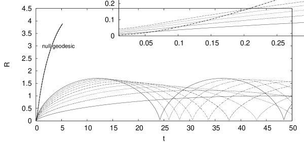
Figure 4: The curves $R({\cal M},t)$ corresponding to several values of ${\cal M}$. The mass increases uniformly from $x=0.01$ on the lowest curve to $x=0.1$ on the highest curve. The origin $t=R=0$ is the point singularity discussed in Sec. 7. A null cone with the vertex at the point singularity is also shown – as can be seen, by the time the outermost mass shell reaches its maximal size, it is within the future light cone of the singularity. The inset shows the light cone in a small neighbourhood of its vertex – all mass shells enter this cone soon after going through the bounce. The region $u<0$, as follows by comparison with Fig. 7, would occupy a very small neighbourhood of the origin and would not be visible at the scale of this figure.

The other qualitative conclusions presented in Paper I remain unchanged. Below, we present the new results found in the present paper. In all the subsequent figures, the radial coordinate $r$ was defined as $r=N^{1/3}$, so that one can instantly see whether there is a central singularity ($R,_{r}=0$ at the center) or not ($R,_{r}>0$ at the center). Fig. 5 shows the functions $u(x)$ and $R,_{r}(x)$ (left graph) and the energy density $\epsilon(x)$ (right graph) in the surface $R=R_{+}$. The functions $u(x)$ and $R,_{r}(x)$ have a zero at the same value of $x$ and opposite signs in all other points, except at $x=0$ where $R,_{r}\to 0$ and $u<0$, so $u/R,_{r}\to-\infty$. As follows from the calculations in Secs. 4 and 7, in this surface the energy density is negative in a vicinity of the center and goes to $-\infty$ at the center.

The fact that the point where $u=0=R,_{r}$ does not seem to be singular is rather mysterious because it is a limiting point of the contour $R,_{r}=0$ in the $(t,x)$-plane, and the rest of the contour is a shell crossing (see Fig. 7), where the energy density does go to $\pm\infty$. But the curves in Fig. 4 are all for smaller values of $x$, so the singularity is not in its range.

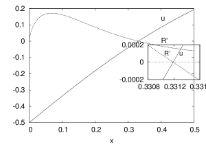
Figure 5: The functions $u(x)$ and $R,_{r}(x)$ (left graph) and energy density $\epsilon(x)$ (right graph) in the surface $R=R_{+}$. The first two change their signs at the same value of $x$, which causes that $u/R,_{r}<0$ in this whole surface, implying $\epsilon<0$ in the whole surface. The inset in the left graph shows the neigbourhood of the intersection point. Note that $R,_{r}\to 0$ at $r\to 0$, which causes the singularity at the center. As shown in Secs. 4 and 7, the energy density in this surface is negative in a vicinity of the center and goes to $-\infty$ at the center.

Fig. 6 shows the functions $u(x)$ and $R,_{r}(x)$ (left graph) and the energy density $\epsilon(x)$ (right graph) in the surface $R=R_{-}$. Within this surface $u(x)$ and $R,_{r}(x)$ are everywhere positive. The energy density is everywhere positive and finite (it does not tend to zero, but to a small positive value as $r\to 0$, as shown in the inset).

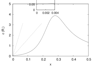
Figure 6: The functions $u(x)$ and $R,_{r}(x)$ (left graph) and energy density $\epsilon(x)$ (right graph) in the surface $R=R_{-}$. The functions $u(x)$ and $R,_{r}(x)$ are positive everywhere, implying $\epsilon>0$ in the whole surface. This time $R,_{r}>0$ at $r=0$, i.e. there is no singularity at the center – as confirmed in the right graph. The inset in the right graph shows that the energy density at the center is not zero, but has a small positive value.

Fig. 7 shows the curves $u=0$ (lower part) and $R,_{r}=0$ (upper part) in the $(t,x)$-plane (actually, each curve is one half of the full contour, which is mirror-symmetric with respect to the $x$-axis). The function $u$ is negative to the left of the lower contour and positive to the right of it. The function $R,_{r}$ is negative to the left of the upper contour and positive to the right of it. As stated above, the set $R,_{r}=0$ is a shell crossing. Its presence proves that the 9 necessary conditions listed at the end of Sec. 2 were not sufficient. Note the characteristic features of the curves, consistent with the calculations of Secs. 4 and 5:

1. The lower curve hits the $t$-axis (the center of symmetry) at $t=0$ (in the figure, we chose $t_{B}=0$, so $t=0$ is the simultaneously achieved state of minimal size). Thus $u$ remains positive all the time as we proceed toward $t=0$ along the center of symmetry.

2. This curve intersects the $x$-axis at some $x>0$. This intersection point coincides with the point where the $u(x)$ and $R,_{r}(x)$ curves intersect in Fig. 5. The upper curve begins at the same point.

3. To the right of the lower curve, we have $u>0$, and to the right of the upper curve $R,_{r}>0$. The energy density is positive in the area to the right of both curves, and negative to the left of any of them, including the $x$-axis.

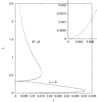
Figure 7: The $u=0$ and $R,_{r}=0$ curves in the $(t,x)$ plane. Each of the functions $u$ and $R,_{r}$ is negative to the left of its graph and positive everywhere to the right. The full contour is mirror-symmetric with respect to the $x$-axis. The $R,_{r}=0$ curve is the locus of shell crossings. The inset shows a closeup view of the neighbourhood of the origin – to demonstrate that the $u=0$ curve hits the $t$-axis only at $t=0$. Thus, at the center of symmetry, $u>0$ everywhere except at the singular origin (where its value becomes dependent on the path of approach). See more explanation in the text.

In order to better visualise the variation of the functions $u$, $R,_{r}$ and $\epsilon$ in the $(t,R)$-plane, we provide three further graphs. Fig. 8 shows the functions $u(x)$ and $R,_{r}(x)$ along the line $t=0.004$ in Fig. 7. Fig. 9 shows the energy density along the same section. It changes sign every time when the line $t=0.004$ crosses one contour or the other. Where $u=0$, it changes from negative to positive by smoothly going through zero; where $R,_{r}=0$ it changes sign by jumping from $+\infty$ to $-\infty$ or the other way round.

Figure 8: The functions $u(x)$ and $R,_{r}(x)$ along the line $t=0.004$ in Fig. 7. The left graph presents these functions for larger values of x, the graph on the right for smaller values of x. Note that $u$ increases to a positive value at the center $x=0$, even though it is negative in a vicinity of the center.

Figure 9: The energy density $\epsilon(x)$ along the line $t=0.004$ in Fig. 7. The left graph presents $\epsilon(x)$ for large values of x, the graph on the right for small values of x. Note, in the left graph, that the curve goes through zero as it crosses the $u=0$ contour, but very near to that point it crosses the $R,_{r}=0$ contour which is a shell crossing. There, it goes to $+\infty$ on one side and to $-\infty$ on the other. The second intersection with $R,_{r}=0$ is also seen at $x\approx 2$, where the density changes sign again by a jump from $-\infty$ to $+\infty$. The right graph shows how the density becomes negative with very large absolute value in a vicinity of the center at $x=0$, but then, still closer to the center, grows to very large positive values.

Fig. 10 shows the same functions along the line $t=t_{2}$, where $t_{2}$ lies between $t=0.004$ and the right end of the the $u=0$ contour in Fig. 7; $t_{2}=0.025$. Finally, Fig. 11 shows the functions $u(x)$, $R,_{r}(x)$ and $\epsilon(x)$ along the line $t=t_{3}$, where $t_{3}$ lies completely to the right of the $u=0$ contour in Fig. 7. In each case, the functions behave exactly in the way in which Fig. 7 implies they should.

Figure 10: The functions $u(x)$ and $R,_{r}(x)$ (left graph) and the energy density $\epsilon(x)$ (right graph) along the line $t=0.025$ in Fig. 7.

Figure 11: The functions $u(x)$, $R,_{r}(x)$ and $\epsilon(x)$ along the line $t=0.05$ in Fig. 7.

Fig. 13 of Paper I, which showed the schematic Penrose diagram of the evolution of our exemplary model, is still qualitatively correct. However, now it has to be supplemented with a few new elements – the images of the surfaces $u=0$ and the light cone of the point singularity at the center. The complete version of that diagram is shown in Fig. 12, and here is the explanation.

Figure 12: A schematic Penrose diagram for the configuration defined by eqs. (8.1) – (8.2) and (8.5). The image of the interior of the dust ball is deformed to make its center $R=0$ coincide, wherever possible, with the set $r=0$ of the background Reissner – Nordström diagram – this is why the null geodesics there are not straight lines at $45^{\circ}$. See more explanation in the text.

The diagram is written into the background of the Penrose diagram for the maximally extended Reissner–Nordström spacetime (thin lines). C is the center of symmetry, Sb is the surface of the charged ball, S_RN is the Reissner–Nordström singularity. The interior of the body is encompassed by the lines C, E, Sb and B; the only singularity that occurs within this area is the point singularity at the center, marked PS. The dotted lines issuing from PS mark the approximate position of the future and past light cone of the singularity (i.e. the Cauchy horizon of the nonsingular part of the surface $R=R_{+}$). Lines B and E connect the points in spacetime where the shell crossings occur at different mass shells. N1 (N2) are the past- (future-) directed null geodesics emanating from the points in which the shell crossings reach the surface of the body (compare Fig. 4). The line Sb should be identified with the uppermost curve in Fig. 4. The top end of Sb is where the corresponding curve in Fig. 4 first crosses another curve, the middle point of Sb is at $t=0$ in Fig. 4. The two dotted arcs marked “$u$” symbolise the hypersurfaces $\epsilon=0$, on which the energy density changes from positive (below the lower curve) to negative and then to positive again (above the upper curve). The distance between these arcs is greatly exaggerated; at the proper scale of the figure they would seem to coincide. The arcs are parts of the $u=0$ contour shown in Fig. 7. In Figs. 4 and 12, the surface of the body is at smaller $x$ than the top of the $u=0$ contour in Fig. 7. Every $N\neq 0$ world line of the dust necessarily enters the region of negative energy density for a finite time interval around the instant of maximal compression.

9 Permanent avoidance of singularity is impossible

In Paper I we hypothesised that a permanently nonsingular configuration of charged dust might exist – provided the period of oscillations is independent of the mass ${\cal M}$. We show below that in our class of configurations the period cannot be independent of ${\cal M}$ because conditions (1) – (9) prohibit this.

The condition $T_{c,{\cal M}}=0$, if considered by explicitly differentiating (2.29), leads to a very complicated integral equation that we were not able to handle. (The integral in (2.29) cannot be explicitly calculated without knowing the explicit form of $C({\cal M},R)$.) However, let us recall that both $T_{p}$ given by (2.28) and $T_{c}$ given by (2.29) are in general functions of ${\cal M}$ only. Thus, we conclude that $T_{c}$ is a function of $T_{p}$, and so the condition for the special case of $T_{c}$ being constant is

$$\frac{{\rm d}{T_{c}}}{{\rm d}{\cal M}}=\frac{{\rm d}{T_{c}}}{{\rm d}{T_{p}}}\frac{{\rm d}{T_{p}}}{{\rm d}{\cal M}}=0.$$ (9.1)

Hence, $T_{c}$ will be constant when

$$\frac{{\rm d}{T_{p}}}{{\rm d}{\cal M}}=0\Longleftrightarrow\frac{{\rm d}{T_{p}}}{{\rm d}{N}}=0,$$ (9.2)

since (2.21) implies that $N,_{\cal M}\neq 0$. From (2.28), (2.9) and $T_{p}=C=$ const we then find

$$(-2E)^{3/2}\equiv\left(1-\Gamma^{2}\right)^{3/2}=C^{3/2}\left({\cal M}-QQ,_{N}\Gamma\right).$$ (9.3)

From here

$$QQ,_{N}=-\frac{1}{\Gamma}\left(\frac{1-\Gamma^{2}}{C}\right)^{3/2}+\frac{\cal M}{\Gamma}.$$ (9.4)

Given $\Gamma(N)$ and ${\cal M}(N)$ found from (2.21), this determines $Q(N)$ simply by integration.

We now verify whether (9.4) is consistent with the regularity conditions (2.22) – (2.25) and the 9 conditions listed after (2.30).

From (2.28) we see that $T_{p}=C=$ const implies

$$\lim_{{\cal M}\to 0}\frac{M}{\cal M}=\frac{D^{3/2}C}{2\pi},$$ (9.5)

where, as stated after (2.5), $D$ may be zero. Then, comparing (2.23) with (2), we see that

$$\lim_{{\cal M}\to 0}\frac{M}{(-2E){\cal M}^{1/3}}=\alpha\neq 0,\qquad\alpha<\infty,$$ (9.6)

where $\alpha$ is a constant. This, together with (2.25), means

$$\lim_{{\cal M}\to 0}\frac{M}{D{\cal M}}=\alpha<\infty,$$ (9.7)

i.e. that $D\neq 0$. But with $CD\neq 0$, eq. (9.5) is in contradiction with $\lim_{{\cal M}\to 0}M/{\cal M}\neq 0$ (see the remark at the end of Sec. 2).

We have thus proven that a configuration with $E<0$ cannot pulsate with the period of pulsations being independent of the mass ${\cal M}$, while being singularity-free for ever. Different periods for different mass shells will necessarily cause shell crossings, during the second cycle at the latest (Fig. 4 illustrates this).

Permanently nonsingular oscillations of weakly charged dust, with the period independent of mass, are possible only when there is a central singularity. An example of such a configuration results when $\Gamma=1/\cosh(bx)$, where $b$ is a constant.

A spherically symmetric charged dust configuration can be permanently nonsingular only if it is static. Such configurations do indeed exist with special forms of the arbitrary functions, as pointed out in Refs [4] and [1], but they are not interesting from the point of view of avoiding singularities.

10 Conclusions

The conclusion of this paper is: the weakly charged spherically symmetric dust distribution considered here (${Q,_{N}}^{2}<G/c^{4}$ at $N>0$ and ${Q,_{N}}^{2}=G/c^{4}$ at $N=0$) must contain at least one of the following features:

1. A Big Bang/Big Crunch singularity;

2. A permanent central singularity;

3. A shell crossing singularity in a vicinity of the center

4. A finite time interval around the bounce instant in which the energy density becomes negative, and a transient momentary singularity of infinite energy density at a single point on the world line of the center of symmetry.

A fully nonsingular bounce is possible for a strongly charged configuration, ${Q,_{N}}^{2}>G/c^{4}$, which can exist only with $E>0$ – see the comments after (2.14). This would be a collapse followed by a single bounce and re-expansion to infinite size. This phenomenon occurs also in the Newtonian limit – the bounce here is caused by the prevalence of electrostatic repulsion over gravitational attraction. Such an example was reportedly found, but never published, by Ori and coworkers [6].

A permanently nonsingular pulsating configuration of spherically symmetric charged dust does not exist. At most, a single full cycle of nonsingular bounce can occur, and shell crossings will necessarily appear during the second collapse phase. The nonsingular bounce occurs at $R>0$, but the momentary isolated singularity at the center of symmetry is still there.

The possibility of $\epsilon$ going negative in the presence of electric charges does not seem to have been noticed and may need further work on its interpretation. If the negative energy density region existed permanently in some part of the space, with comoving boundary, then we might suspect that this is a consequence of a bad choice of parameters that implies unphysical properties in that region. However, here we have the case in which the energy density is positive for some time, and then these same matter particles acquire negative energy density in a time-interval around the bounce instant. This suggests that there is some physical process involved in this, which should be further investigated.

A question arises now. The uncharged limit of the family of configurations defined by eqs. (2.1) – (2.10), $Q=0$, is the Lemaître – Tolman (L–T) model [8, 9]. For the latter, shell crossings can be avoided, as is well-known since long ago [10]. Why, then, are they unavoidable with $Q\neq 0$?

The answer is this: in the L–T model, the Big Bang (BB) or Big Crunch (BC) are unavoidable (both are present when $E<0$). In the cases that are colloquially called “free of shell crossings”, in reality the shell crossings are not removed, but shifted to the epoch before the BB or after the BC, or both. Thus, the shell crossings are no longer in the domain of physical applicability of the model. When the BB/BC singularities are replaced with a smooth bounce in charged dust, the shell crossings that were hidden on the other side of BB/BC become physically accessible, and they terminate the evolution of the configuration.

Appendix A The proof that $R_{+}(N)$ coincides with $H_{\rm min}(N)$ at the local extrema of $H_{\rm min}(N)$

We stated in the caption to Fig. 10 in Paper I, that the curves $H_{\rm min}(N)$ and $R_{+}(N)$ were not really tangent at the point where $H_{\rm min}(N)$ has its maximum, but just close to one another. In fact, they not only were tangent at that point, but had to be tangent, independently of the explicit forms of the two functions. We show here that this is a general law: at every local extremum of $H_{\rm min}(N)$ (call it $N_{e}$) we have $H_{\rm min}(N_{e})=R_{+}(N_{e})$.

The radius of the inner R–N horizon as a function of $N$ is

$$H_{\rm min}(N)={\cal M}-\sqrt{{\cal M}^{2}-GQ^{2}/c^{4}},$$ (A.1)

where ${\cal M}$ and $Q$ are assumed to depend on $N$ through $x=N/N_{0}$. We do not assume any explicit form of the functions ${\cal M}$ and $Q$, we only use the general properties (2.9), (2.15) and (2.23).

At every local extremum $N=N_{e}$ we have $H_{{\rm min},N}=0$. Using (2.23), this means

$$\left[\Gamma\sqrt{{\cal M}^{2}-GQ^{2}/c^{4}}\right]_{e}=\left[{\cal M}\Gamma-QQ,_{N}\right]_{e},$$ (A.2)

where the subscript $e$ denotes the value at the extremum. From here

$$\left[\frac{GQ^{2}}{c^{4}}\right]_{e}=\left[\frac{QQ,_{N}}{\Gamma^{2}}\left(2{\cal M}\Gamma-QQ,_{N}\right)\right]_{e}.$$ (A.3)

Substituting this value of $GQ^{2}/c^{4}$ in (A.1) wet get

$$H_{\rm min}(N_{e})=QQ,_{N}/\Gamma.$$ (A.4)

Substituting the same value of $GQ^{2}/c^{4}$ in (2.13) for $R_{+}$ we find

$$R_{+}(N_{e})=QQ,_{N}/\Gamma=H_{\rm min}(N_{e}).$$ (A.5)

$\square$

Appendix B Proof of (3.2)

For simplicity, to avoid physical coefficients, we introduce the functions $p(x)$, $\mu(x)$ and $F_{2}(x)$ (where $x=N/N_{0}$, $N_{0}=$ const) by

$$Q(N)\ {\overset{\rm def}{=}}\ \pm\frac{\sqrt{G}N_{0}}{c^{2}}\ p(x),\qquad{\cal M}\ {\overset{\rm def}{=}}\ \frac{GN_{0}}{c^{4}}\ \mu(x)\qquad M(N)\ {\overset{\rm def}{=}}\ \frac{GN_{0}}{c^{4}}\ F_{2}(x).$$ (B.1)

Then, to prove (3.2) we must prove that

$$\lim_{x\to 0}\left[-2Ep^{2}\left({p,_{x}}^{2}-1\right)\right]/{F_{2}}^{2}=0.$$ (B.2)

By condition (5), in a vicinity of $x=0$, $p$ must be of the form

$$p(x)=x+A_{p}x^{\alpha_{p}}+{\cal O}_{\alpha_{p}},\Longrightarrow{p,_{x}}^{2}-1=2A_{p}x^{\alpha_{p}-1}+{\cal O}_{\alpha_{p}-1},$$ (B.3)

where $A_{p}$ and $\alpha_{p}>1$ are constants, and ${\cal O}_{\alpha_{p}}$ is an unspecified function with the property $\lim_{x\to 0}{\cal O}_{\alpha_{p}}/x^{\alpha_{p}}=0$. Then, by the regularity condition (2.24),

$$\Gamma=1+A_{E}x^{\alpha_{E}}+{\cal O}_{\alpha_{E}}\Longrightarrow-2E=-2A_{E}x^{\alpha_{E}}+{\cal O}_{\alpha_{E}},$$ (B.4)

where $\alpha_{E}\geq 2/3$, by (2.25). It follows from (2.21) and (2.8) – (2.9) that

$$\mu(x)=x+A_{m}x^{\alpha_{E}+1}+{\cal O}_{\alpha_{m}}.$$ (B.5)

Hence,

$$F_{2}\equiv\mu-pp,_{x}\Gamma=\left(A_{m}-A_{E}\right)x^{\alpha_{E}+1}-A_{p}\left(\alpha_{p}+1\right)x^{\alpha_{p}}-{\cal O}_{\alpha_{p}}-{\cal O}_{\alpha_{E}+1}.$$ (B.6)

Thus $F_{2}$ is of order $\alpha_{p}$ or $\alpha_{E}+1\geq 5/3$, whichever limit is lower. However, the limit via $\alpha_{E}$ leads to a central singularity, since then, from (2), $R/N^{1/3}\to 0$ as $N\to 0$, so (2.23) will not hold. Consequently, $F_{2}$ is of order $\alpha_{p}$, while the second term under the square root in (3.1), $-2Ep^{2}\left({p,_{x}}^{2}-1\right)$ is of order $\alpha_{2}=\alpha_{E}+\alpha_{p}+1$. Suppose that $\alpha_{2}\leq 2\alpha_{p}$, so that the second term under the square root in (3.1) is of lower order than the first one. This translates to $\alpha_{p}\geq\alpha_{E}+1$. But condition (2.23), in combination with (2), requires that $\alpha_{p}=\alpha_{E}+1/3$, or else a central singularity will appear. Thus, $-2Ep^{2}\left({p,_{x}}^{2}-1\right)$ must be of higher order in $x$ than ${F_{2}}^{2}$ in eq. (3.1), i.e. (3.2) must hold. $\square$

Now consider the case when we approach the center of symmetry along the locus of the outer turning points, $R=R_{-}$. Then $u_{-}=\Gamma-QQ,_{N}/R_{-}$ remains positive up to the center, as is seen from the reasoning below. The conclusion that $-2Ep^{2}\left({p,_{x}}^{2}-1\right)$ is of higher order in $x$ than ${F_{2}}^{2}$ still applies, so we have

$$\lim_{N\to 0}u_{-} \equiv \lim_{N\to 0}\left[\Gamma+\frac{2EQQ,_{N}}{M+\sqrt{M^{2}-2EQ^{2}\left({Q,_{N}}^{2}-G/c^{4}\right)}}\right]$$ (B.7)

$$= 1+Q,_{N}(0)\lim_{N\to 0}EQ/M=1+Q,_{N}(0)\lim_{x\to 0}Ep/F_{2}.$$

We know from the above that $p(x)=x+A_{p}x^{\alpha_{p}}+{\cal O}_{\alpha_{p}}$, $F_{2}=-A_{p}\left(\alpha_{p}+1\right)x^{\alpha_{p}}-{\cal O}_{\alpha_{p}}$ and $E=A_{E}x^{\alpha_{E}}+{\cal O}_{\alpha_{E}}$, while the regularity condition (2.23) implies, via (2), that $\alpha_{E}=\alpha_{p}-1/3$. This, taken together, implies that $\lim_{x\to 0}Ep/F_{2}=0$, i.e. that $\lim_{N\to 0}u_{-}=1>0$, i.e. that $u_{-}$ remains positive up to the very center.

Appendix C Impossibility of a vacuole around $R=0$ with $E<0$

Let us assume $E(x)$ as in (B.4) and $p(x)$ in a form similar to (B.3):

$$p(x)=\alpha x+A_{p}x^{\alpha_{p}}+{\cal O}_{\alpha_{p}},\Longrightarrow p,_{x}=\alpha+A_{p}\alpha_{p}x^{\alpha_{p}-1}+{\cal O}_{\alpha_{p}-1},$$ (C.1)

For the function $\mu(x)$ this implies

$$\mu=x+\frac{A_{E}}{\alpha_{E}+1}x^{\alpha_{E}+1}+{\cal O}_{\alpha_{E}+1}.$$ (C.2)

Then

$$F_{2}(x) \equiv \mu-pp,_{x}\Gamma=\left(1-\alpha^{2}\right)x-A_{E}\left(2\alpha^{2}-\frac{1}{\alpha_{E}+1}\right)x^{\alpha_{E}+1}-\alpha A_{p}\left(\alpha_{p}+1\right)x^{\alpha_{p}}$$ (C.3)

$$+ {\cal O}_{\alpha_{p}}+{\cal O}_{\alpha_{E}+1}.$$

Now we have two cases: $\alpha^{2}\neq 1$ and $\alpha^{2}=1$. In the first case we have $F_{2}=\left(1-\alpha^{2}\right)x+{\cal O}_{1}(x)$. Thus, in order that $M/E$ has a nonzero limit at $x\to 0$, it follows that $\alpha_{E}=1$. Then, if the terms $(M/2E)^{2}$ and $Q^{2}\left({Q,_{N}}^{2}-G/c^{4}\right)/(2E)$ in (2.13) are to be of the same order, the ratio $p^{2}\left({p,_{x}}^{2}-1\right)/(2E)$ should have a nonzero finite limit at $x\to 0$. But, with $\alpha^{2}\neq 1$ and $\alpha_{E}=1$ we have

$$\frac{p^{2}\left({p,_{x}}^{2}-1\right)}{2E}=\frac{x^{2}\left(\alpha+A_{p}x^{\alpha_{p}-1}+{\cal O}_{\alpha_{p}-1}\right)^{2}\left(\alpha^{2}-1+2A_{p}\alpha_{p}x^{\alpha_{p}-1}+{\cal O}_{\alpha_{p}-1}\right)}{2A_{E}x+{\cal O}_{1}}$$

$$\ {\underset{x\to 0}{\longrightarrow}}\ 0,$$ (C.4)

which has the consequence that $R_{+}=0$, i.e. the conditions $Q={\cal M}=0$ cannot be imposed at $R>0$.

In the second case, $\alpha^{2}=1$, we can assume $\alpha=1$ (nothing in the equations depends on the sign of $Q$); then $F_{2}$ is of the order of either $x^{\alpha_{E}+1}$ or $x^{\alpha_{p}}$, whichever exponent is smaller. With $\left(\alpha_{E}+1\right)$ being smaller, the result is immediately seen: If $F_{2}$ is of the order $x^{\alpha_{E}+1}$ while $E$ is of the order $x^{\alpha_{E}}$, then $\lim_{x\to 0}M/E=0$, and $\lim_{x\to 0}R_{+}=0$. With $\alpha_{p}$ being smaller we have

$$\frac{p^{2}\left({p,_{x}}^{2}-1\right)}{2E}=\frac{x^{\alpha_{p}+1}\left(1+A_{p}x^{\alpha_{p}-1}+{\cal O}_{\alpha_{p}-1}\right)^{2}\left(2A_{p}\alpha_{p}+{\cal O}_{0}\right)}{2A_{E}x^{\alpha_{E}}+{\cal O}_{\alpha_{E}}}.$$ (C.5)

This will have a finite limit at $x=0$ if $\alpha_{E}=\alpha_{p}+1$. But we are considering the case when $F_{2}$ is of order $x^{\alpha_{p}}$, which means that the limit of $F_{2}/E$, i.e. the limit of $M/E$ at $x\to 0$ will be infinite, which again shows that the matching conditions cannot be fulfilled at a finite nonzero $R$. $\square$

Acknowledgement We are grateful to the referee for pointing out several errors in an earlier version of this paper.

References

- [1] A. Krasiński, K. Bolejko, Phys. Rev. D73, 124033 (2006) + erratum Phys. Rev. D75, 069904 (2007). Corrected version: gr-qc 0602090.
- [2] A. Ori, Class. Q. Grav. 7, 985 (1990).
- [3] A. Ori, Phys. Rev. D44, 2278 (1991).
- [4] J. Plebański and A. Krasiński, An Introduction to General Relativity and Cosmology. Cambridge University Press 2006.
- [5] P. A. Vickers, Ann. Inst. Poincarè A18, 137 (1973).
- [6] A. Ori, private communication.
- [7] A. Krasiński, Gen. Rel. Grav. 33, 145 (2001).
- [8] G. Lemaître, Ann. Soc. Sci. Bruxelles A53, 51 (1933); English translation, with historical comments: Gen. Rel. Grav. 29, 637 (1997).
- [9] R. C. Tolman, Proc. Nat. Acad. Sci. USA 20, 169 (1934); reprinted, with historical comments: Gen. Rel. Grav. 29, 931 (1997).
- [10] C. Hellaby and K. Lake, Astrophys. J. 290, 381 (1985) + erratum in Astrophys. J. 300, 461 (1985).