NUHEP-EX/07-01

An Experiment to Search for Light Dark Matter in Low-Energy $ep$ Scattering Sven Heinemeyer¹, Yonatan Kahn², Michael Schmitt², Mayda Velasco²

¹Instituto de Fisica de Cantabria (CSIC-UC), Santander, Spain
²Northwestern University, Evanston, Illinois, USA December 12, 2007

Abstract Anomalous production of low-energy photons from the galactic center have fueled speculations on the nature and properties of dark matter particles. In particular, it has been proposed that light scalars may be responsible for the bulk of the matter density of the universe, and that they couple to ordinary matter through a light spin-$1$ boson. If this is the case, then such particles may be produced in the quasi-elastic low-energy scattering of electrons off protons. We present a proposal for an experiment to search for this process and assess its viability.

1 Introduction

The INTEGRAL data provide evidence for an anomalous production of low-energy gammas from the galactic center [1]. The excess is largest in the region at and below $E_{\gamma}=511$ keV leading to the conclusion that positron-electron annihilation is responsible. The question becomes: where are the extra positrons coming from? One answer is that they are produced in the annihilation processes of dark-matter particles, which we will write as $\chi\chi^{*}\rightarrow e^{+}e^{-}$, where $\chi$ denotes the dark-matter (DM) particle.

A phenomenological model has been developed which posits a light dark-matter particle $\chi$ and a new spin-1 gauge boson $U$ which mediates interactions between $\chi$ and ordinary matter particles, such as electrons [2]. The couplings of the $U$-boson to standard model fermions is not specified by any theoretical first principles; rather, they are left as parameters to be constrained by the known dark-matter abundance and processes studied in the laboratory. At a minimum, there must be a non-zero coupling to the dark matter particles as well as to electrons, a fact which we exploit in our proposal to observe $U$ bosons in the laboratory.

The experiment we propose makes use of a low-energy electron beam ($E_{\mathrm{beam}}\approx 40~{}{\mathrm{MeV}}$) and a fixed hydrogen gas-jet target. We describe two versions: the first is rather simple and requires a minimum of resources, and the second is more elaborate allowing for a greater sensitivity. We attempt to compare the sensitivity and potential information gained from our proposed experiment to other suggested avenues of research, such as the study of $e^{+}e^{-}$ collision data [3].

This paper is organized as follows. We begin with a brief review of the evidence for the low-energy gamma-ray excess from the galactic center, followed by a resume of the light dark matter models recently discussed in the literature. Next we explain the process of interest in general terms, followed by a detailed description of the two experimental set-ups to study this process. We make a comparison with other proposals followed by a summary of our work.

2 Gamma-Ray Excess

In 1972, Johnson et al. [4] used a balloon-hoisted NaI scintillation telescope to detect a 511 keV line emanating from the center of the galaxy. After accounting for 511 keV radiation resulting from cosmic rays and positron annihilation in the upper atmosphere, they concluded that this line was significantly stronger than the cosmic background radiation from other directions at similar energies. Leventhal et al. [5] revisited this phenomenon in 1978 and identified the source of the radiation as positron annihilation; specifically, they concluded that positrons in the galactic center form both para-positronium, which annihilates to give the 511 keV line, and ortho-positronium which contributes a spectrum of excess low-energy radiation at and below $511$ keV. Further experiments over the past 30 years, and most recently the INTEGRAL satellite, have refined the value of the observed photon flux and identified the majority of the radiation as coming from the galactic bulge [1, 6, 7, 8]. Currently, the explanation of annihilating positronium is well-accepted as the source of the radiation, but the source of the positrons themselves remains unclear. Several possibilities involving relatively well-known astrophysical phenomena have been put forth, including radioactive nuclei from supernovae [9], gamma-ray bursts [10], pulsars [11], black holes [12], and cosmic rays [13], but these models have difficulty accounting for the morphology and high intensity of the photon flux except under rather restrictive assumptions.

To resolve these problems, several more exotic explanations from particle physics have been proposed. A partial list compiled by Sizun et al. [14] includes Q-balls, relic particles, decaying axinos, primordial black holes, color superconducting dark matter, superconducting cosmic strings, dark energy stars, moduli decays, and annihilating light dark matter particles. The latter explanation, in which dark matter particles annihilate in the galactic bulge to form $e^{+}e^{-}$ pairs, has been able to account for both the morphology and intensity of the line as long as the dark matter particles are light ($<100~{}{\mathrm{MeV}}$) [15, 16, 17, 18]. Radiative processes play an important role in comparisons with gamma-ray data, and provide additional constrants on the model [19, 14]. In the past four years, the light dark matter model has been refined to account for the increasingly accurate data from INTEGRAL; the upper limit of the particles’ mass has been placed anywhere from $3$ to $20~{}{\mathrm{MeV}}$ [14, 20, 21, 23] and the theoretical aspects of this model have been studied considerably [17, 24, 25]. In particular, the flux intensity measurements have allowed a fairly accurate determination of the cross-section of the annihilation reaction [25, 27]. Several authors have noted that increasingly accurate measurements of the morphology of the $511$ keV line would allow the mass of the proposed particle to be narrowed down even further [20, 21, 22].

The annihilating dark matter scenario has attracted much attention because it is the easiest “exotic” explanation to test experimentally. For instance, Ref. [28] focused on detecting a line from the galactic center that would result from the dark matter particles annihilating directly to photons, and Ref. [3] proposed searches for the gauge boson involved in annihilation processes at high-energy $e^{+}e^{-}$ colliders. We show that the light dark matter model can be tested cleanly and simply in the laboratory, using techniques and methods that are readily available today. Even taking into account the range of possible dark matter particle mass, the kinematical distinctions between a dark matter production event and background events are clear enough that a signal could be identified with a high degree of confidence. Moreover, if dark matter were to be detected in such an experiment, the measurement of the cross-section would allow an independent check of the parameters in the light dark matter model, and by extension, provide significant information on the annihilations that take place at the center of the galaxy.

3 Resume of the Light Dark Matter Model

If the positron excess is explained by $\chi\chi^{*}\rightarrow e^{+}e^{-}$, then clearly there is an effective $e^{+}e^{-}\chi\chi^{*}$ vertex. Calculations by Boehm, Fayet and others have linked the strength of this effective vertex to the observed dark matter abundance, and the dark matter particle mass, $M_{\chi}$. The $e^{+}e^{-}\chi\chi^{*}$ interaction would be modeled by one or more intermediate particles. According to a recent paper [25], one needs both a heavy fermion called the $F^{\pm}$ and a light neutral vector boson called the $U$ to explain both the primordial abundance of dark matter and the current rate of positron annihilation in the galactic center. In this model, the dark matter particles are neutral scalars with masses on the order of $1$–$10~{}{\mathrm{MeV}}$. There are other models in which $\chi$ is a fermion [26], but for concreteness, we will take $\chi$ to be a scalar. The $U$-boson is also light, with $M_{U}>2M_{\chi}$ and $M_{U}<100~{}{\mathrm{MeV}}$, and it decays mainly to $\chi\chi^{*}$. The mass of the $F^{\pm}$ fermion is at least several hundred GeV and plays no role in our process, so we do not consider it further. Feynman diagrams for the dark matter annihilation are given in Fig. 1.

The experiment that we propose does not depend crucially on these assumptions. Rather, this phenomenological model serves as a guide for gauging the sensitivity of our experiment. In order to estimate rates for our signal process, we must specify the coupling constants. We follow a recent paper by Fayet [29], which links this model to several experimental data, as well as a paper by Ascasibar, et al. [25], which links the model to various astrophysical data. According to Ascasibar et al., the $U$ boson plays the dominant role in fixing the primordial abundance of dark matter, while the $F^{\pm}$ fermion controls the present day rate of annihilations, and hence the rate of positron production. Fayet uses the dark matter abundance to constrain the $U$-boson couplings and does not hypothesize a heavy $F^{\pm}$ fermion. He shows how particle physics data constrain the $U$-boson couplings as a function of its mass. Despite these differences, both papers report similar constraints on the coupling constants of the $U$ boson to the dark matter particles, $C_{\chi}$, and to electrons, $f_{e}$. Other publications placing similar constraints include [2, 24, 30, 31].

If the dark matter abundance is used to constrain the $U$-boson couplings, then

$$|C_{\chi}f_{e}|\approx 10^{-6}\frac{M_{U}^{2}-4M_{\chi}^{2}}{M_{\chi}\,(1.8~{}{\mathrm{MeV}})}\,\sqrt{B^{ee}_{\mathrm{ann}}}$$ (1)

where $B^{ee}_{\mathrm{ann}}$ is the fraction of all $\chi\chi^{*}$ annihilations which result in an $e^{+}e^{-}$ final state (see Eq. (57) in Ref. [29]). We will assume that $B^{ee}_{\mathrm{ann}}=1$, although a lower value is possible if there is a significant coupling of the $U$-boson to neutrinos. If $\chi$ were a spin-$1/2$ fermion, then this formula would be modified by a factor ${\cal{O}}(1)$. Since our aim is to assess the viability of an experiment, however, we will neglect any such factors in this paper. Fig. 2 (TOP) depicts this constraint as a function of $M_{\chi}$ for three choices of $M_{U}$. The single dot shows our default choice of model on which our rate estimates in Sec. 4 are based. Fig. 2 (BOTTOM) shows the constraint from Eq. (1) as a function of $M_{U}$, for three choices of $M_{\chi}$. It also shows the upper bounds on $|C_{\chi}f_{e}|$ derived by Fayet from three lepton-based experimental measurements, namely, the measurement of $(g-2)_{e}$ [32], the measurement of $(g-2)_{\mu}$ [33], and the $\nu-e$ cross-section measurement [34]. These constraints apply to the vector coupling of the $U$-boson to the electron; more stringent constrains apply to the axial coupling. We will set the axial coupling to zero in our calculations. The constraint from $\nu-e$ scattering assumes that $f_{\nu}=f_{e}$ and will be weaker if $f_{\nu}\ll f_{e}$. The constraint from $(g-2)_{\mu}$ applies to our process only for $f_{\mu}=f_{e}$. Fayet also derives constrains from $\psi$ and $\Upsilon$ decays, as well as atomic parity violation experiments, but we will assume that the $U$-boson couples to leptons only.

Figure 1: dark matter annihilation into an $e^{+}e^{-}$ pair, through $U$-boson exchange in the $s$-channel, and $F^{\pm}$-fermion exchange in the $t$-channel

Figure 2: TOP: constraints on $C_{\chi}f_{e}$ as a function of $M_{\chi}$, for three values of $M_{U}$. BOTTOM: heavy red lines show constraints on $C_{\chi}f_{e}$ as a function of $M_{U}$, for three values of $M_{\chi}$. The thinner dashed blue lines show constraints coming from the measurements of $(g-2)_{\mu}$, $(g-2)_{e}$ and $\sigma(\nu e)$ (see text), from Ref. [29], and we have set $C_{\chi}=1$. The hook-shaped green curve indicates the sensitivity of the first experimental design, discussed in Sec. 5.1. The dots indicate our default choice for masses and couplings.

4 Low-Energy Quasi-Elastic $ep$-Scattering

We wish to exploit the different kinematic characteristics of the signal process

$$e^{-}p\rightarrow e^{-}p\,U^{(*)}\rightarrow e^{-}p\,\chi\chi^{*}$$

and of simple elastic scattering

$$e^{-}p\rightarrow e^{-}p$$

at low energy. The kinematics of the scattered electron and proton are highly constrained for elastic scattering, and much less so for the signal process. Several kinematic distinctions can be made, which allows an efficient and effective discrimination of the two processes on the basis of kinematics alone.

Feynman diagrams for the signal process are given in Fig. 3. It is important to note that the same set of vertices appear in both our signal process and the dark matter annihilation process (Fig. 1). Consequently, our signal process must occur if this model is correct, and the signal cross-section can be related directly to the dark-matter annihilation rates in the early universe (which determines the dark matter relic density) and today (which determines the strength of the $511$ keV gamma-ray line from the galactic center).

Figure 3: example Feynman diagrams for the signal process. We consider only the $U$-boson diagrams in our estimates; the $F^{\pm}$-fermion diagrams can be neglected.

Since the dark matter particles are light, by hypothesis, we choose to employ a low electron beam energy which essentially closes off all inelastic processes, leaving only elastic scattering as a significant background process. For example, we may take an electron beam of energy $E_{\mathrm{beam}}\approx 40~{}{\mathrm{MeV}}$ and a fixed hydrogen target, for which $\sqrt{s}\approx M_{p}+E_{\mathrm{beam}}<M_{p}+M_{\pi}$, since $E_{\mathrm{beam}}\ll M_{p}$. There can be no inelastic background from ordinary strong-interaction processes, and if a pure hydrogen target is used, there would be no nuclear excitations, either.

A very small background will come from the process $e^{-}p\rightarrow e^{-}p\nu\bar{\nu}$ mediated by an off-shell $Z$ boson. The Feynman diagram is the same as the $U$-boson exchange diagram (Fig. 3), with the $U$-boson replaced by a virtual $Z$-boson and the scalar particles $\chi\chi^{*}$ replaced by $\nu\bar{\nu}$. This background process is completely negligible – about nine orders of magnitude smaller than the hypothetical signal – since $M_{U}\ll M_{Z}$.

Higher-order QED radiative processes $e^{-}p\rightarrow e^{-}p\gamma(\gamma)$ also pose a background. They occur at a smaller rate than elastic scattering. The final-state photons tend to emerge along the directions of the incoming and outgoing electrons, and hence do not change their directions [35], although a small component of “wide-angle” Bremsstrahlung can occur and has been observed in muon-scattering experiments [36]. Calculations for experiments at HERA and JLAB show extremely small rates outside a cone of $0.1$ rad [37]. In the case that the radiated photons emerge along the scattered electron direction, they can be detected together with the scattered electron. If they are emitted along the beam direction, thereby reducing the effective $\sqrt{s}$ for the $ep$ interaction, the correlation of the electron and proton directions changes very little. This is a special feature of our kinematical situation, in which $M_{p}\gg E_{\mathrm{beam}}\gg M_{e}$. Additionally, QED radiation peaks at low photon energies, which means that the deviation of the scattered electron energy from the lowest-order results tends to be small, with no sharp kinematic features. The signal process peaks at large deviations, and there are distinctive kinematic features due to the phase space needed to produce two dark-matter particles, and/or an on-shell $U$-boson. Finally, the QED radiation pattern varies very little with the beam energy, while the signal process will have a strong dependence. Hence, discrimination between the signal process and QED radiative processes will be possible if the signal rate is not too small.

The concept for the experiment is the following: collide a well-defined electron beam onto a hydrogen target, and observe the scattering angle and energy of the outgoing electrons and protons. For ordinary elastic scattering, the energy of the scattered electron emerging at a given angle is constrained to a unique value. So one would look for events with a significantly lower energy as evidence for the production of a final state that is lighter than a single pion. Confirmation for an anomalous final state would come from the measurement of the scattering angle and energy of the outgoing proton. The kinematic distributions for the final-state electron and proton would allow, in principle, a confirmation of the production of light invisible scalars of a particular mass, as opposed to the production of a pair of neutrinos. In the absence of a signal, stringent limits could be placed on the masses and effective couplings of dark matter to electrons.

The keys to identifying signal events are:

1. For a given scattering angle, the scattered electron will have a much lower energy than in elastic scattering.

2. The outgoing proton will be relatively slow; for elastic scattering the proton is energetic.

3. For a given electron scattering angle, the scattering angle of the proton will vary over a wide range. In elastic scattering, the proton emerges at a unique angle.

4. The electron and proton can be acoplanar for the signal event, due to the momentum taken by the $\chi\chi^{*}$ pair; for elastic scattering the electron and proton are strictly back-to-back in the transverse plane, even if there is final-state radiation.

5. The signal will increase rapidly as $E_{\mathrm{beam}}$ is increased from threshold, while elastic scattering decreases as $1/E_{\mathrm{beam}}^{2}$. There will be a minimum beam energy corresponding to the threshold for producing two dark-matter particles, below which there is no signal.

6. The signal cross-section is less sharply peaked toward small electron scattering angles.

7. In principle, the $U$ boson may decay to an electron-positron pair rather than the invisible $\chi\chi^{*}$ state. The final topology would contain four charged tracks. If the $U$-boson is on mass shell, then the mass distribution of the ‘extra’ $e^{+}e^{-}$ pair would give a peak at the $U$-boson mass. If it is off mass shell, then the mass distribution will be less sharply peaked toward $2M_{e}$ than that due to photon conversions.

These very distinctive features allow an efficient selection of events with very little background. As described later in this paper, a simple apparatus should allow signal events to be identified at the rate of one event in a ten billion elastic scatters, and a more sophisticated apparatus should achieve a sensitivity better than $10^{-12}$ of the elastic scattering rate. Such experiments should easily cover the range of possible models of this type, leading either to the discovery of the $U$-boson or the exclusion of this and similar models.

While we have based our calculations on a fairly specific model and final state, our argument is not dependent on this model in all of its details. As already noted, the $\chi$ particle might be a fermion instead of a scalar. Furthermore, the experiment we propose could be viewed as the direct production of $U$-bosons, regardless of how they decay or whether they play any role in dark matter phenomena. In this case, the rates would not depend at all on the coupling $C_{\chi}$, and the final states might be dominated by other light particles. If a signal for an anomlous invisible final state were observed, then follow-on experiments would be needed to confirm the connection with dark matter (see Ref. [38]). In order to provide a clear and consistent framework for our discussion, however, we will follow fairly closely the light dark matter model described above.

We proceed now to a discussion of the rates.

4.1 Kinematics

We remind the reader of the basic kinematics for elastic scattering in order to frame our discussion and define our notation. The target proton is effectively at rest in the laboratory frame with four-momentum $P_{\mu}=(M,0,0,0)$, and the incoming beam electron is highly relativistic with four-momentum $p_{\mu}=(E,0,0,p)$. The outgoing electron has $p^{\prime}_{\mu}=(E^{\prime},p^{\prime}\sin\theta,0,p^{\prime}\cos\theta)$ which defines the electron scattering angle $\theta$. The outgoing proton has $P^{\prime}_{\mu}$ and the four-vector of both dark-matter particles we will write as $W_{\mu}$. Hence, $W_{\mu}=p_{\mu}+P_{\mu}-p^{\prime}_{\mu}-P^{\prime}_{\mu}$, and $W_{\mu}=0$ for elastic scattering. For the signal process, $\min(W_{\mu}W^{\mu})=4\,M^{2}_{\chi}$.

Following decades-old convention, we define the four-momentum transferred $q_{\mu}=p^{\prime}_{\mu}-p_{\mu}$ and $Q^{2}=-q^{2}$. To a very good approximation, $Q^{2}=4EE^{\prime}\sin^{2}\theta/2$. The energy transfered in the lab frame is $\nu=E-E^{\prime}$. The kinematic condition for elastic scattering, $P^{\prime 2}=P^{2}=M^{2}$, implies $Q^{2}\approx 2M\nu$, after neglecting a small term proportional to $m_{e}^{2}$.

4.2 Elastic Cross-Section

The elastic electron-proton scattering cross-section, for relativistic electrons is

$$\frac{d\sigma}{d\Omega}=\frac{\alpha^{2}\hbar^{2}c^{2}}{4E^{2}\sin^{4}(\theta/2)}\left(\frac{E^{\prime}}{E}\right)[G_{1}(Q^{2})\cos^{2}(\theta/2)+2\tau G_{2}(Q^{2})\sin^{2}(\theta/2)]$$ (2)

where $\tau=Q^{2}/4M^{2}$ and

$$G_{1}(Q^{2})=\frac{G_{E}^{2}+\tau G_{M}^{2}}{1+\tau},\hskip 8.53581ptG_{2}(Q^{2})=G_{M}^{2}$$

are functions of the proton electric form factor $G_{E}$ and magnetic form factor $G_{M}$. At our low beam energies, $\tau\ll 1$, so we can neglect the magnetic form factor. $G_{E}$ is approximated by the standard dipole fit

$$G_{E}(Q^{2})\approx\left(\frac{\beta^{2}}{\beta^{2}+Q^{2}}\right)^{2},$$

where $\beta=$ 710 MeV. Under these conditions, Eq. (2) simplifies to

$$\frac{d\sigma}{d\Omega}=\frac{\alpha^{2}\hbar^{2}c^{2}}{4E^{2}\sin^{4}(\theta/2)}\left(\frac{E^{\prime}}{E}\right)\left(\frac{\beta^{2}}{\beta^{2}+Q^{2}}\right)^{4}\cos^{2}(\theta/2).$$

$E^{\prime}$ and $\theta$ are related by

$$E^{\prime}=\frac{E}{1+(E/M)(1-\cos\theta)}.$$

The contribution of the form factor to the cross-section is on the order of a few percent at low beam energies; this correction is necessary to get an accurate estimate of the elastic background, but is not needed for an order-of-magnitude estimate of the signal process.

4.3 Signal Cross-Section

We investigated the signal process in two ways. First, we performed a semi-analytic calculation in which the matrix element was assumed to be independent of all momenta. Then we employed CompHEP [39] and implemented the $U$-exchange process, an example of which is shown in the left-hand Feynman diagram of Fig. 3.

4.3.1 Semi-Analytical Cross-section

To get a rough idea of the signal kinematics, we calculated $d^{2}\sigma/d\Omega\,dE^{\prime}$ assuming that the matrix element of the signal process is independent of all momenta. The phase-space calculation for a $2\rightarrow 4$ process can be rather involved, especially when several of the final-state particles are massive, and finding an analytic expression for $d^{2}\sigma/d\Omega\,dE^{\prime}$ in terms of the four-vectors of all outgoing particles is not possible in general. We simplified the calculation by writing $W_{\mu}$ for the sum of the two four-vectors of the scalar particles and expressing the cross-section in terms of the combined invariant mass $W^{2}$ and the combined spatial velocity $\vec{W}$, treating these two quantities as separate variables. In the calculations that follow, all energies and momenta pertain to the center-of-mass frame.

We begin with the Golden Rule for $2\rightarrow 3$ scattering:

$$d\sigma = |\mathcal{M}|^{2}\frac{1}{4\sqrt{(p\cdot P)^{2}-(m_{e}M)^{2}}}\left[\left(\frac{d^{3}\vec{p^{\prime}}}{(2\pi)^{3}2E^{\prime}}\right)\left(\frac{d^{3}\vec{P^{\prime}}}{(2\pi)^{3}2E^{\prime}_{p}}\right)\left(\frac{d^{3}\vec{W}}{(2\pi)^{3}2E_{W}}\right)\right]$$

$$\times(2\pi)^{4}\delta^{4}(p\ +P\ -p^{\prime}\ -P^{\prime}\ -W)$$

where the relevant four-vectors are defined in Section 4.1. Since we are only concerned with the shape of the phase space distribution, we will drop all numerical constants for the rest of this calculation. Making the standard approximation of a massless electron, we integrate out the proton momentum and the angular part of $\vec{W}$, using the delta function to obtain limits on $|\vec{W}|$:

$$|\vec{W}|_{\pm}=\frac{FE^{\prime}\pm(E_{\mathrm{tot}}-E^{\prime})\sqrt{F^{2}-4W^{2}E_{\mathrm{tot}}(E_{\mathrm{tot}}-2E^{\prime})}}{2E_{\mathrm{tot}}(E_{\mathrm{tot}}-2E^{\prime})},$$ (3)

where $E_{\mathrm{tot}}$ is the total energy, $E^{\prime}$ is the outgoing electron energy, and $F\equiv E_{\mathrm{tot}}^{2}+W^{2}-2E_{\mathrm{tot}}E^{\prime}-M^{2}$. At this point

$$\frac{d^{2}\sigma}{d\Omega\,dE^{\prime}}\propto\int_{|\vec{W}|_{-}}^{|\vec{W}|_{+}}\frac{|\vec{W}|}{\sqrt{W^{2}+|\vec{W}|^{2}}}\,d|\vec{W}|=\sqrt{W^{2}+|\vec{W}|_{+}^{2}}-\sqrt{W^{2}+|\vec{W}|_{-}^{2}}.$$ (4)

Requiring that $|\vec{W}|_{\pm}$ be real, i.e., that the term under the radical in (3) be non-negative, gives the upper bound

$$(W^{2})_{+}=M^{2}+E_{\mathrm{tot}}^{2}-2E_{\mathrm{tot}}E^{\prime}-2M\sqrt{E_{\mathrm{tot}}^{2}-2E_{\mathrm{tot}}E^{\prime}}$$

with the lower bound $(W^{2})_{-}=4M_{\chi}^{2}$. We use these bounds to integrate the right-hand side of Eq. (4) over $W^{2}$. It turns out that this integrand can be very well approximated by a square root function:

$$f(W^{2})\equiv\sqrt{W^{2}+|\vec{W}|_{+}^{2}}-\sqrt{W^{2}+|\vec{W}|_{-}^{2}}\approx K\sqrt{(W^{2})_{+}-W^{2}}.$$

The normalization constant $K$ is chosen so that the square root function matches $f(W^{2})$ at the endpoint $W^{2}=(W^{2})_{-}$; that is,

$$K=\frac{f((W^{2})_{-})}{\sqrt{(W^{2})_{+}-(W^{2})_{-}}}\ ;\hskip 5.69054ptf(W^{2})\approx\frac{f((W^{2})_{-})}{\sqrt{(W^{2})_{+}-(W^{2})_{-}}}\sqrt{(W^{2})_{+}-W^{2}}.$$

(The other endpoint $W^{2}=(W^{2})_{+}$ is already taken care of since both the square root and $f(W^{2})$ vanish there.) Performing the integration over $W^{2}$, we now have

$$\frac{d^{2}\sigma}{d\Omega\,dE^{\prime}} \propto \int_{(W^{2})_{-}}^{(W^{2})_{+}}\frac{f((W^{2})_{-})}{\sqrt{(W^{2})_{+}-(W^{2})_{-}}}\sqrt{(W^{2})_{+}-W^{2}}\ d\,(W^{2})$$

$$\propto f((W^{2})_{-})\,((W^{2})_{+}-4M_{\chi}^{2})$$

$$= \left(\sqrt{4M_{\chi}^{2}+|\vec{W}|_{+}^{2}}-\sqrt{4M_{\chi}^{2}+|\vec{W}|_{-}^{2}}\right)((W^{2})_{+}-4M_{\chi}^{2})$$

where $|\vec{W}|_{\pm}$ are evaluated at $(W^{2})_{-}=4M_{\chi}^{2}$.

A plot of this function, boosted from the CM frame to the lab frame, gives the broad phase-space curves in Fig. 7. We note that this calculation is model-independent in the sense that it makes no reference to the nature of the interaction.

4.3.2 CompHEP Calculations

We implemented $U$-boson exchange between electrons and dark matter particles. An example Feynman diagram is shown on the left side of Fig. 3. The proton was represented as a massive fermion with no internal structure, which, for the very low beam energies we propose, is a very good approximation. The mass of the dark matter particle was set to $M_{\chi}=2~{}{\mathrm{MeV}}$, and the mass of the $U$-boson was set to $M_{U}=10~{}{\mathrm{MeV}}$. Hence, the $U$-boson was produced on mass shell. The coupling of the $U$-boson is assumed to be purely vectorial – see Fig. 4 for the Feynman rules for the $U$-$\chi$ and $U$-$e$ vertices. We imposed the relic abundance constraint, Eq. (1). Taking $C_{\chi}=1$ and $B^{ee}_{\mathrm{ann}}=1$, this gives $f_{e}\approx 2.3\times 10^{-5}$.

Figure 4: Feynman rules for the $U$-$\chi$ and $U$-$e$ vertices

For the purposes of this paper, we set the beam energy to $E_{\mathrm{beam}}=40~{}{\mathrm{MeV}}$, and we considered a narrow range of electron scattering angle $89.4^{\circ}<\theta_{e}<90.6^{\circ}$, which follows from the conceptual design presented in Section 5.1.

The mass of the $U$-boson is not well constrained. If the product of coupling constants $C_{\chi}f_{e}$ is held fixed, then the signal cross-section drops rapidly as a function of $M_{U}$, as depicted by the solid curve in Fig. 5 (TOP). The presence of the threshold at $M_{U}\approx 40~{}{\mathrm{MeV}}$ is evident. If the $M_{U}$ boson were heavier, then one would run this experiment at a higher beam energy. Backgrounds will not increase so long as $E_{\mathrm{beam}}<135~{}{\mathrm{MeV}}$, and in fact the signal cross-section will increase, up to a certain point. According to Eq. (1), the constraints $C_{\chi}f_{e}$ should be adjusted as a function of $M_{U}$. The result for the cross-section is shown as the dashed curve, which is much flatter than the solid curve, showing that the rate of this process is indeed tied directly to the rate of dark matter annihilation. Fig. 5 (BOTTOM) shows the variation of the signal cross-section as a function of beam energy, for three choices of $M_{U}$. A typical threshold behavior is evident.

Figure 5: signal cross-sections. TOP: accepted cross-section as a function of $M_{U}$. The solid line shows the result with a fixed coupling constant, and the dashed line shows the result when the constant varies with mass according to Eq. (1). Here, “accepted” refers to a limited angular range for the scattered electron: $89.4^{\circ}<\theta<90.6^{\circ}$. BOTTOM: cross-section as a function of the beam energy, for three values of $M_{U}$, as indicated. The curves for $M_{U}=5~{}{\mathrm{MeV}}$ and $20~{}{\mathrm{MeV}}$ have been multiplied by factors of $20$ and $0.2$, respectively.

Figure 6: differential signal cross-sections as a function of angles. TOP: $d\sigma/d\Omega$ plotted as a function of $\cos\theta$. The elastic scattering cross-section has been scaled down by a factor of $10^{-10}$. BOTTOM: $d\sigma/d\theta_{p}$ showing the broad distribution expected for the signal. The vertical dashed lines show the very narrow range expected for elastic scattering even allowing for radiative processes.

Since the signal process is inelastic, the electron is scattered at larger angles than for the background process – see Fig. 6 (TOP). Clearly the ratio of signal to background is a strong function of the scattering angle, and so we have chosen $\theta=90^{\circ}$, as an example. An optimized choice of $\theta$ would depend on $M_{U}$ as well as the details of the apparatus, which is beyond the scope of this paper.

The wide range of proton scattering angles, $\theta_{p}$, is also a distinctive feature of the signal process. Fig. 6 (BOTTOM) shows $d\sigma/d\theta_{p}$, with the electron scattering angle $\theta_{e}$ constrained as above. The dashed lines indicate the narrow range of $\theta_{p}$ expected for elastic scattering. This range does not change even when the incoming electron emits an energetic photon during the scattering process.

An important feature of the signal process is the reduced energy of the outgoing electron. For $E_{\mathrm{beam}}=40~{}{\mathrm{MeV}}$ and $\theta=90^{\circ}$, perfect elastic scattering gives $E^{\prime}=38.4~{}{\mathrm{MeV}}$. For the signal process, $E^{\prime}$ follows a much broader distribution with a peak at rather low values, as shown in Fig. 7. It is an interesting feature of quantum field theory that a massless spin-$1$ boson, such as the photon, is emitted with an energy that peaks toward the minimum possible value, while a massive spin-$1$ boson, such as the $U$-boson considered here, is emitted with a momentum that peaks toward the maximum possible value. Thus the CompHEP calculation, based on the matrix element for $U$-boson exchange, shows a scattered electron energy distribution which peaks toward small values. The phase-space calculation, described in Section 4.3.1, sets the matrix element to a constant, resulting in a broader distribution for the scattered electron energy as shown in Fig. 7.

On the basis of these CompHEP calculations, and for $89.4^{\circ}<\theta_{e}<90.6^{\circ}$, the accepted signal cross-section is $2.13\times 10^{-4}~{}{\mathrm{pb}}$, and the cross-section for elastic scattering is $8.0\times 10^{5}~{}{\mathrm{pb}}$, which gives a ratio of cross-sections of $2.7\times 10^{-10}$. We checked these results using CalcHEP [40]. In the next section we describe experiments which should be able to probe this range successfully, and either establish the existence of this signal process or rule it out definitively.

Figure 7: signal shapes compared to a Gaussian centered at $E^{\prime}=38.4~{}{\mathrm{MeV}}$ with an r.m.s. of $6\%$ (see text). Two examples of phase-space distributions are shown, for $M_{\chi}=2~{}{\mathrm{MeV}}$ and $9~{}{\mathrm{MeV}}$ (see Sec. 4.3.1). One example of a CompHEP matrix-element calculation is shown, for $M_{\chi}=2~{}{\mathrm{MeV}}$ and $M_{U}=10~{}{\mathrm{MeV}}$ (see Sec. 4.3.2).

5 Proposed Experiments

The two proposed experiments bring a low-energy electron beam ($E_{\mathrm{beam}}=40~{}{\mathrm{MeV}}$) onto a fixed hydrogen target, and record a large number of elastic scattering events. Each design exploits kinematic differences as discussed in Section 4 above. The first design is simple and is meant to demonstrate the concept, while the second is somewhat more ambitious, though easily within the capabilities of existing techniques.

5.1 Experimental Design I

This design exploits the correlations between the scattering angle and outgoing electron energy, and the proton angle and velocity. Fixing the electron scattering angle in a narrow range $89.4^{\circ}<\theta<90.6^{\circ}$, the other three quantities should be centered in narrow ranges around certain values, namely, scattered electron energy $E^{\prime}=38.4~{}{\mathrm{MeV}}$, scattered proton momentum $P^{\prime}_{p}=55.4~{}{\mathrm{MeV}}$, and angle $\theta_{p}=43.8^{\circ}$. We imagine that the electron is detected in a high-resolution electromagnetic calorimeter placed at $\theta=90^{\circ}$ and covering $2\pi$ in azimuth, and the proton is detected in a Silicon strip detector placed at $\theta_{p}=43.8^{\circ}$. Elastic scattering would give a coincidence in the calorimeter and Silicon detectors. The calorimeter would measure the energy of the electron, and the silicon would measure the kinetic energy of the proton due to its very high $dE/dX$, since $v\sim 10^{-3}c$ for the proton.

A redundant measurement of the proton velocity would come from measuring its time-of-flight across a fixed distance. We present this time-of-flight as a function of the proton momentum in Fig. 8, where the dot indicates the expected value $P^{\prime}_{p}=55.4~{}{\mathrm{MeV}}$ for elastic scattering. The resolution on the proton momentum worsens as the momentum increases. Nonetheless, for a distance $d=2$ m, and for a time-of-flight resolution of $2$ ns, the measurement uncertainty on $P^{\prime}_{p}$ would be only $1~{}{\mathrm{MeV}}$, which is more than adequate for these purposes.

The energy resolution of the calorimeter is of paramount importance. Recent examples of high-resolution electromagnetic calorimetry based on high-purity single crystals suggest that a resolution of about $6\%$ could be achieved for $E^{\prime}=38.4~{}{\mathrm{MeV}}$ [41]. Fig. 7 compares a purely Gaussian peak centered on this value for $E^{\prime}$ with an r.m.s. of $6\%$ to three signal distributions generated according to the phase space model, and the matrix-element calculation. The Gaussian curve is normalized to unity and the three signal shapes are normalized to $10^{-10}$.

A clear separation between signal and background from the elastic peak is evident, and in this simple picture it is easy in principle to isolate a signal by requiring $E^{\prime}<20~{}{\mathrm{MeV}}$, for example. This cut would retain more than 75% of the signal, while the Gaussian is effectively removed.

The signal from elastic scattering will not correspond exactly to a Gaussian, however, due to resolution effects in the calorimeter and due to radiative processes mentioned in Section 4. It is beyond the scope of this paper to try to estimate the exact shape of the elastic scattering peak. One should note that many of the radiated photons will be emitted along the direction of the outgoing electron, and hence will strike the same calorimeter element that the scattered electron does. This element will therefore register the energy radiated by the electron together with the photon, providing a kind of automatic correction for the radiation. If photons are emitted by the incoming electron resulting in an effective radiative energy loss for the interaction, the energy of the outgoing electron and proton decrease proportionally, as shown in the top plot of Fig. 9. However, the angle of the outgoing proton hardly changes at all, as shown in the bottom plot of Fig. 9. Consequently, a robust signal for elastic scattering is available. Radiation emitted at wide angles is extremely rare, perhaps on the order of $10^{-6}$ [37], and in principle could be tagged.

Scattering from residual gas molecules which have migrated far from the nominal interaction point might mimic the kinematics of the signal, and thereby constitute a background that is not easy to reject on the basis of our kinematic cuts. An assessment of the level of this background requires a detailed design and perhaps some level of proto-typing, which is beyond the scope of this paper.

It is difficult to estimate the power of this apparatus to reject elastic scattering. Nonetheless, it may be plausible that our signal could be isolated from elastic scattering. The signature would be an outgoing electron at low $E^{\prime}$ values (well below $25~{}{\mathrm{MeV}}$) and either the absence of a proton, or a slow proton exiting at an angle significantly different from $44^{\circ}$ (see bottom plot of Fig. 5), and with an azimuthal angle with respect to the electron different from $180^{\circ}$. QED radiative processes would not give a peak at low $E^{\prime}$, rather, they would produce a tail to the Gaussian peak shown in Fig. 7. The variation of any signal with $E_{\mathrm{beam}}$ and $\theta$ is quite different from the variation of the background (see Fig. 5 (BOTTOM) and Fig. 6 (TOP)).

Figure 8: time-of-flight for the outgoing proton, when it traverses a distance of two meters. The dot marks the expected momentum for elastic scattering in experimental design I.

Figure 9: the impact of radiative energy loss due to photons emitted by the incoming electron on the kinematics of elastic scattering. TOP: the momentum of the outgoing particles. BOTTOM: the variation of the proton scattering angle $\theta_{p}$.

As a toy example, we imagine an incoming beam with $E=40~{}{\mathrm{MeV}}$ and a current of 10 mA. It impinges on a gas-jet hydrogen target with a density of $\rho=2\times 10^{18}$ atoms/cm² [42]. Our calorimeter consists of one ring of elements arrayed at $\theta=90^{\circ}$, as shown in Fig. 10. The calorimeter elements are single high-purity PbWO₄ crystals shaped as regular polyhedra which project toward the target. The front face might be 2 cm $\times$ 2 cm, and the elements might be placed $1$ m from the target. We assume a Gaussian resolution of 6%, or $2.4~{}{\mathrm{MeV}}$ at $38~{}{\mathrm{MeV}}$ [41]. Additional plastic scintillator would be used to indicate when a shower has leaked laterally outside the crystals, and when a wide-angle photon has been emitted. The proton is detected with a silicon strip detector placed at the angle expected for elastic scattering. Additional detectors could be placed at other angles to confirm a proton scattered in the signal process. The experimental region would be filled with a low-$Z$ material, such as Helium gas, to minimize multiple scattering and energy loss of the proton.

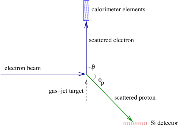
Figure 10: experimental design I

We integrated Eq. 2 numerically to obtain an accepted cross-section for this simple apparatus, and obtained $0.8~{}\mu$b. With the stated beam current and target density, the rate of elastic scatters is $2\times 10^{5}$ events/s. With two months’ good running time (10 hours per day for fifty days), one would accumulate on the order of $10^{11}$ elastic scattering events.

An accurate estimate of the sensitivity of this experiment to our signal process would require detailed simulations of the apparatus, radiative and other energy loss processes. We cannot provide such an estimate at this time. However, a rough order-of-magnitude estimate can be made as follows. Fig. 7 shows a very clear kinematic distinction based on the measured scattered electron energy. A simple cut such as $E^{\prime}<20~{}{\mathrm{MeV}}$ amounts to $8\sigma$ below the elastic peak. For an ideal calorimeter, none of the $10^{11}$ elastic scatters would survive this, while $>75\%$ of the signal would survive, depending on $M_{\chi}$. In practice, this simple cut on $E^{\prime}$ would be reinforced by the powerful cuts on the outgoing proton. A positive signal of $15$ events would correspond to a signal cross-section that is a about factor of $2\times 10^{-10}$ smaller than the elastic scattering cross-section, or about $0.2$ fb. The absence of any signal would correspond to an upper limit of about $3\times 10^{-5}$ pb, for our default choice of coupling constants and masses. We can estimate how such an upper limit would vary as a function of $M_{U}$, and the result is shown as the hook-shaped curve in Fig. 5. Apparently, this simple apparatus has a good chance to observe a signal or rule out this model.

If a signal were observed in the energy spectrum of the scattered electron, then one could expand the coverage of the Silicon detector so that the recoil proton would be well measured for signal events. Then the kinematics of the initial state and the outgoing electron and proton would be known on an event-by-event basis, and it would be possible to measure the mass of the invisible final state by computing the recoil mass. Specifically, with our definition of the missing four-momentum, $W_{\mu}=p_{\mu}-p^{\prime}_{\mu}+P_{\mu}-P^{\prime}_{\mu}$, the invariant mass of the two dark-matter particles would be $M_{\chi\chi}^{2}=W_{\mu}W^{\mu}$. There will be a threshold of $2M_{\chi}$ for $\sqrt{W_{\mu}W^{\mu}}$, and if the $U$-boson is produced on mass shell, then there will be a peak at $\sqrt{W_{\mu}W^{\mu}}=M_{U}$. A detailed simulation is needed in order to understand the resolution of the recoil mass.

5.2 Experimental Design II

This design augments the calorimetry of the first design with an open-geometry tracking device and a magnetic field. Precise measurements of the momenta and direction of the outgoing electron and proton would provide powerful handles against background processes. As pointed out in Section 4, there are angular variables which can be exploited to identify a signal. Furthermore, such measurements serve to verify the electron energy as measured by the calorimeter and thereby reduce radiative backgrounds.

We envision a cylindrical geometry coaxial with the beam – see Fig. 11. The region around the target would be instrumented with two layers of precision silicon detectors which would provide the position and angles of the outgoing electron and proton. For the sake of discussion, we take the radii of these two cylinders to be $1.5$ cm and $2.5$ cm. It is likely that the inner cylinder could be reduced to a few mm, depending on the properties of the beam. Directly outside the second cylinder we generate a toroidal magnetic field. A small number of conducting rods will run parallel to the beam and carry a modest current. A circumferential magnetic field is generated with a strength on the order of hundreds of Gauss. This field bends the electron and proton but they remain co-planar with the beam, which is important for triggering and data analysis. At a radius of 1 m, we install a cathode strip or multi-wire proportional chamber to measure the $z$-coordinates of the electron and proton. This measurement together with the initial trajectory measured by the silicon detectors gives us the momenta of the two particles. Another set of conducting rods carries a current which terminates the magnetic field. Finally, an extended version of the calorimeter measures the energy of the scattered electron, independently of the tracking system, as well as any photons radiated away from the beam.

All of the proposed detector elements are ordinary, and many examples exist in working detectors. The scale of the apparatus is modest, as is the number of instrumented channels. The event rate would be rather low compared to modern high-energy physics experiments, so read-out electronics would not need to be especially fast.

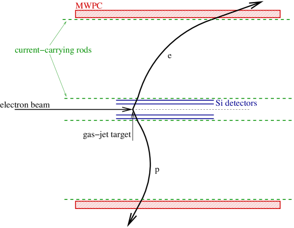
Figure 11: experimental design II

5.2.1 Analysis Plan

The measurements $z_{0},z_{1},z_{2}$ of the electron position at the surfaces of the three nested cylinders allow an accurate identification of a dark matter production event. The accuracy of this analysis plan depends significantly on the properties of the silicon detectors used at the surfaces of the inner two cylinders; in particular, there is an absolute “worst-case” error $\Delta z$ in the measurement of position, on the order of $100~{}\mu$m. In the following discussion we suppose that the incoming electron beam is traveling along the $z$-axis in the positive direction. For a given event, we compute the measured scattering angle $\theta_{\mathrm{meas}}$ from $z_{0},z_{1}$, and the distance $R_{1}-R_{0}$ between the two inner cylinders. We then simulate the path of the electron assuming the event was an elastic collision, obtaining the outgoing electron energy from the kinematics of the reaction, and find the expected position $z^{\prime}_{2}$ at the outer detector wires. At this point all events with $z_{2}<z^{\prime}_{2}$ are rejected.

If the event were in fact an elastic collision, and $\theta_{\mathrm{meas}}>\theta_{\mathrm{true}}$, then $z_{2}>z^{\prime}_{2}$ and such an event would survive the first cut. To eliminate these remaining elastic events, we consider the worst-case scenario when $\theta_{\mathrm{meas}}$ is too large; that is, where there are measurement errors of $+\Delta z$ at $R_{0}$ and $-\Delta z$ at $R_{1}$. In this situation, our “worst-case” value of $\theta_{\mathrm{true}}$ is computed using $z_{0}-\Delta z$ and $z_{1}+\Delta z$, instead of $z_{0}$ and $z_{1}$. We then find the outgoing energy for an elastic collision with this scattering angle and repeat the simulation to find the new expected position $z^{\prime\prime}_{2}$. After cutting all events with $z_{2}<z^{\prime\prime}_{2}$, we are guaranteed that no elastic events have survived. For $70^{\circ}<\theta_{\mathrm{true}}<110^{\circ}$, $E_{\mathrm{beam}}=40~{}{\mathrm{MeV}}$, and $M_{\chi}=2~{}{\mathrm{MeV}}$, a simple Monte Carlo simulation shows that the majority of dark matter production events survive the cuts.

5.2.2 Rates and Sensitivity

The rate of elastic events would scale up from what was discussed in Section 5.1 due to the much larger solid angle covered. Also, one would presumably employ a more intense beam and/or thicker target. We imagine that on the order of $10^{14}$ elastic scattering events would be recorded, giving a sensitivity on the order of $10^{-8}~{}{\mathrm{pb}}$. More importantly, a large sample of signal events could be detected, allowing a real measurement of the cross-section and of the mass of the $U$-boson.

5.2.3 Threshold Behavior

Fig. 5 (BOTTOM) shows the excitation curves for our signal process. Our default beam energy, $E_{\mathrm{beam}}=40~{}{\mathrm{MeV}}$, is close to the maximum cross-section when $M_{U}=10~{}{\mathrm{MeV}}$. With the larger event samples expected in this more sophisticated experimental design, one could measure the cross-section as a function of $E_{\mathrm{beam}}$, and trace out the threshold behavior. Fig. 5 indicates that even just three modest measurements at $E_{\mathrm{beam}}=40~{}{\mathrm{MeV}}$, $20~{}{\mathrm{MeV}}$ and $80~{}{\mathrm{MeV}}$ would allow one to distinguish clearly between the three mass values $M_{U}=10~{}{\mathrm{MeV}}$, $20~{}{\mathrm{MeV}}$ and $5~{}{\mathrm{MeV}}$. Furthermore, experimental design II would allow a measururement of the angular variation of the signal process. As shown in Fig. 6 (TOP), a clear distinction with respect to elastic scattering could be made.

5.2.4 Other Signatures

Returning to the light dark matter model, we recall that the intermediate particles ($U$-boson and/or $F^{\pm}$-fermions) couple to electrons, and hence the process

$$e^{-}p\rightarrow e^{-}p\,e^{+}e^{-}$$

must occur (see Fig. 12). The invariant mass of the extra $e^{+}e^{-}$ pair would peak at the $U$-boson mass. If the electron coupling $f_{e}$ is not too low, then one might obtain a sample of such events, which would be easy to distinguish from any other process. The observation and measurement of all final-state particles would allow an incisive study of this model. The prediction for the rate of this process, however, is more model dependent, since it depends on $f_{e}^{2}$ rather than $C_{\chi}f_{e}$, and is less constrained by the dark-matter abundance, Eq. (1).

Figure 12: Feynman diagram for $e^{+}e^{-}$ pair production via a $U$ boson

5.3 Comparison to $e^{+}e^{-}$-Scattering

A classic study of invisible final states has been carried out at $e^{+}e^{-}$ colliders. The idea is to tag the event by the presence of a wide-angle photon radiated from the incoming electron or positron. Recently, Borodatchenkova et al. proposed using this process to detect light dark matter [3]. Also, Zhu discussed the possibility of making an observation at BES III [43], and claims a sensitivity down to $f_{e}\sim 10^{-5}$.

Our proposal benefits in a number of ways. First, the luminosity is much higher due to the use of a fixed target. Second, the kinematics are particularly advantageous, since at tree-level there are no backgrounds and elastic scattering is highly constrained. Finally, the recoil mass can be used to measure the $U$-boson mass, in principle.

6 Summary and Conclusions

The light dark matter model proposed by Boehm and Fayet can explain both the relic density of dark matter and the 511 keV gamma-ray line coming from the center of the galaxy. It survives many constraints derived from precision measurements in particle physics, and also several astrophysical observations. The key ingredients of this model include a stable light neutral scalar, $\chi$, and a light neutral vector boson $U$ with a large coupling to $\chi$ and a small coupling to electrons.

We propose a simple experiment to produce the $U$-bosons in low-energy electron-proton scattering. Basically, the $U$-boson would be radiated from the incoming electron, resulting an invisible final state which can be identified through dramatic kinematical differences with respect to elastic scattering. The high luminosity and easy control of the kinematics should allow the experiment to reach a sensitivity which would confirm or definitively rule out this model. Two conceptual designs are described, which will be modeled and studied in greater detail in the future.

7 Acknowledgments

We wish to thank Céline Boehm and David Buchholz for helpful discussions in the initial stages of this study, and Pierre Fayet, John Beacom and David Jaffe for very useful comments after the first version of this paper appeared. S.H. thanks Edward Boos, Rikkert Frederix and Fabio Maltoni for technical assistance. The work of S.H. was partially supported by CICYT (grant FPA2006–02315).

References

-
[1]
P. Jean et al.,
Status of the 511 keV Line from the Galactic Centre Region,
Proceedings of the 5th INTEGRAL Workshop on the INTEGRAL Universe
(ESA SP-552)
16-20 February 2004, Munich, Germany J. Knodsleder et al., Early SPI/INTEGRAL Constraints on the Morphology of the keV Line Emission in the 4th Galactic Quadrant, Astron. Astrophys. 411 (2003) L457 - [2] C. Boehm and P. Fayet, Scalar dark matter candidates, Nucl. Phys. B683 (2004) 219
- [3] Natalia Borodatchenkova, Debajyoti Choudhur and, Manuel Drees, Probing MeV Dark Matter at Low-Energy Colliders, Phys. Rev. Lett. 96 (2006) 141802
- [4] W.N. Johnson III, F. R. Harnden, Jr. and R.C. Haymes, The Spectrum of Low-Energy Gamma Radiation from the Galactic-Center Region, Ap. J. 172 (1972) L1-L7
- [5] M. Leventhal, C.J. MacCallum and P. D. Stang, Detection of 511 keV Positron Annihilation Radiation from the Galactic Center Direction, Ap. J. 225 (1978) L11-L14
- [6] L.X. Cheng, et al., A Maximum Entropy Map of the 511 keV Positron Annihilation Line Emission Distribution near the Galactic Center, Ap. J. (Letters) 481 (1997) L43
- [7] W.R. Purcell, et al., OSSE Mapping of Galactic 511 keV Positron Annihilation Line Emission, Ap. J. 491 (1997) 725
- [8] G. Vedrenne, et al., SPI: The spectrometer aboard INTEGRAL, Astronomy and Astrophysics 411 (2003) L299
- [9] P. A. Milne, J. D. Kurfess, R. L. Kinzer and M. D. Leising, Supernovae and Positron Annihilation Radiation, New Astron. Rev. 46 (2002) 553
- [10] G. Bertone, A. Kusenko, S. Palomares-Ruiz, S. Pascoli and D. Semikoz, Gamma ray bursts and the origin of galactic positrons, Phys. Lett. B636 (2006) 20
- [11] P. A. Sturrock, A Model of Pulsars, Ap. J. 164 (1971) 529
- [12] R. Ramaty and R. E. Lingenfelter, Gamma-ray evidence for a stellar-mass black hole near the Galactic center, New York Academy of Sciences Annals 571 (1989) 433
- [13] B. Kozlovsky, R.E. Lingenfelter and R. Ramaty Positrons from accelerated particle interactions. Ap. J. 316 (1987) 801
- [14] P. Sizun, M. Casse and S. Schanne, Continuum gamma-ray emission from light dark matter positrons and electrons, Phys. Rev. D74 (2006) 063514
- [15] C. Boehm, T.A. Ensslin and J. Silk, Can annihilating Dark Matter be lighter than a few GeVs?, J. Phys. G30 (2004) 279
- [16] Celine Boehm, Dan Hooper, Joseph Silk and Michel Casse, MeV Dark Matter: Has It Been Detected?, Phys. Rev. Lett. 92 (2004) 101301
- [17] C. Boehm, P. Fayet and J. Silk, Light and Heavy Dark Matter Particles, Phys. Rev. D69 (2004) 101302
- [18] Celine Boehm and Yago Ascasibar, More evidence in favour of Light Dark Matter particles?, Phys. Rev. D70 (2004) 115013
-
[19]
J. F. Beacom, N. F. Bell and G. Bertone,
Gamma-ray constraint on Galactic positron production by MeV dark matter,
Phys. Rev. Lett. 94, 171301 (2005);
J. F. Beacom and H. Yuksel, Stringent Constraint on Galactic Positron Production, Phys. Rev. Lett. 97, 071102 (2006);
- [20] Kyungjin Ahn and Eiichiro Komatsu, Dark Matter Annihilation: the origin of cosmic gamma-ray background at 1-20 MeV, Phys. Rev. D72 (2005) 061301
- [21] Shinta Kasuya and Masahiro Kawasaki, 511 keV line and diffuse gamma rays from moduli, Phys. Rev. D73 (2006) 063007
- [22] Y. Rasera, R. Teyssier, P. Sizun, B. Cordier, J. Paul, M. Casse and P. Fayet, Soft gamma-ray background and light dark matter annihilation, Phys. Rev. D 73, 103518 (2006)
- [23] Le Zhang, Xuelei Chen, Yi-An Lei and Zongguo Si, The impacts of dark matter particle annihilation on recombination and the anisotropies of the cosmic microwave background, Phys. Rev. D74 (2006) 103519
- [24] Pierre Fayet, U-boson detectability, and Light Dark Matter LPTENS-06/24, arXiv:hep-ph/0607094; ibid., Phys. Rev. D74 054034 (2006)
- [25] Y. Ascasibar, P. Jean, C. Boehm and J. Knoedlseder, Constraints on dark matter and the shape of the Milky Way dark halo from the 511 keV line, Mon. Not. Roy. Astron. Soc. 368 (2006) 1695
- [26] P. Fayet, Light spin-1/2 or spin-0 dark matter particles, Phys. Rev. D 70, 023514 (2004)
- [27] Pierre Fayet, Dan Hooper and Gunter Sigl, Constraints on Light Dark Matter From Core-Collapse Supernovae, Phys. Rev. D73 (2006) 063007
- [28] C. Boehm, J. Orloff and P. Salati, Light Dark Matter Annihilations into Two Photons, Phys. Lett. B641, 247 (2006)
- [29] Pierre Fayet, -boson Production in Annihilations, and Decays, and Light Dark Matter, Phys. Rev. D 75, 115017 (2007); ibid., n The Search For A New Spin 1 Boson, Nucl. Phys. B 187, 184 (1981)
- [30] Chen Jacoby and Shmuel Nussinov, Some Comments on an MeV Cold Dark Matter Scenario, JHEP 0705, 017 (2007)
- [31] Dan Hooper, Manoj Kaplinghat, Louis E. Strigari and Kathryn M. Zurek, MeV Dark Matter and Small Scale Structure, Phys. Rev. D 76, 103515 (2007)
- [32] G. Gabrielse et al., New Determination of the Fine Structure Constant from the Electron g-Value and QED, Phys. Rev. Lett. 97 (2006) 030802
- [33] G. W. Bennett et al., [Muon G-2 Collaboration], Final Report of the Muon E821 Anomalous Magnetic Moment Measurement at BNL, Phys. Rev. D73 (2006) 072003
- [34] L. B. Auerbach et al., [LSND Collaboration], Measurement of electron-neutrino Elastic Scattering, Phys. Rev. D63 (2001) 112001
- [35] Luke W. Mo and Yung-Su Tsai, Radiative Corrections to Elastic and Inelastic ep and p Scattering, Rev. Mod. Phys. 41 (1969) 205
- [36] J. J. Aubert et al., [European Muon Collaboration], A Measurement Of Wide Angle Bremsstrahlung In A High-Energy Muon Scattering Experiment As A Check On The Consistency Of Radiative Correction Calculations, Z. Phys. C10 (1981) 101
- [37] A. A. Akhundov, D. Yu. Bardin and L. V. Kalinovskaya, Electron state Bremsstrahlung processes at HERA, Z.Phys. C51 (1991) 557 K. J. F. Gaemers and M. van der Horst, The Process as a Fast Luminosity Monitor for the HERA Collider, Nucl.Phys. B316 (1990) 269 (Err. B336 184)
- [38] Y. Kahn and M. Schmitt, in preparation
-
[39]
A. Pukhov, et al., [CompHEP Collaboration],
CompHEP - a package for evaluation of Feynman diagrams and
integration over multi-particle phase space. User’s manual for version 3.3,
arXiv:hep-ph/9908288
E. Boos, et al., [CompHEP Collaboration], CompHEP 4.4: Automatic computations from Lagrangians to events, Nucl. Instrum. Meth. A534 (2004) 250 - [40] A. Pukhov, Calchep 3.2: MSSM, structure functions, event generation, 1, and generation of matrix elements for other packages, arXiv:hep-ph/0412191
-
[41]
J. M. Bauer [BaBar Collab.],
The BaBar electromagnetic calorimeter: Status and performance improvements,
IEEE Nucl. Sci. Symp. Conf. Rec. 2, 1038 (2006);
PrimEx experiment at JLAB, Readiness document, Nov 20, 2003,
http://www.jlab.org/primex/documents/
PANDA Experiment (Darmstadt), http://www-panda.gsi.de/ - [42] B.M. Fisher, et al., Improvements to the Gas-Jet Target TUNL Progress Report, XXXIX, 132 (2000)
- [43] Shou-hua Zhu, U-boson at BESIII, Phys. Rev. D 75, 115004 (2007)