ARCRAIDER I: Detailed optical and X-ray analysis of the cooling flow cluster Z3146

We present a detailed analysis of the medium redshift ($z=0.2906$) galaxy cluster Z3146 which is part of the ongoing ARCRAIDER project, a systematic search for gravitational arcs in massive clusters of galaxies. The analysis of Z3146 is based on deep optical wide field observations in the $B$, $V$ and $R$ bands obtained with the WFI@ESO2.2m, and shallow archival WFPC2@HST taken with the $F606W$ filter, which are used for strong as well as weak lensing analyses. Additionally we have used publicly available XMM/Newton observations for a detailed X-ray analysis of Z3146. Both methods, lensing and X-ray, were used to determine the dynamical state and to estimate the total mass. We also identified four gravitational arc candidates.
We find this cluster to be in a relaxed state, which is confirmed by a large cooling flow with nominal $\sim 1600$ M_⊙ per year, regular galaxy density and light distributions and a regular shape of the weak lensing mass reconstruction. The mass content derived with the different methods agrees well within 25% at $r_{200}=1661\;h_{70}^{-1}$kpc indicating a velocity dispersion of $\sigma_{v}=869^{+124}_{-153}$ km/s.

1 Introduction

Galaxy clusters are the largest bound structures in the universe and therefore excellent cosmological probes. In particular, large samples of clusters allow a statistical study of their physical properties. Such samples need clear selection criteria, e.g. selection by mass. Due to the tight relation between the X-ray luminosity $L_{\rm X}$ and the mass (Schindler, 1999; Reiprich & Böhringer, 1999) X-ray surveys provide an excellent basis to select the most massive systems for lensing studies (Luppino et al., 1999; Smith et al., 2001, 2005; Bardeau et al., 2005).
The combination of lensing and X-ray studies allows us to get important insights into galaxy clusters, as it offers the possibility to obtain physical properties of the cluster members, the Intra Cluster Medium (ICM) and the determination of the cluster gravitational mass and its distribution with independent methods.
However, the mass determination of galaxy clusters is a very difficult task. It is dependent on the method adopted and on the validity of the assumptions used to convert observables to cluster masses. Currently two methods are widely used: (a) From the gas density and temperature profiles measured with X-ray observations it is possible to derive an estimate of the gravitational mass by assuming spherical symmetry and hydrodynamical equilibrium (see e.g. Allen et al., 2001, 2002; Ettori & Lombardi, 2003; Pointecouteau et al., 2004; Pratt & Arnaud, 2005; Voigt & Fabian, 2006). (b) The second method is based on gravitational lensing analyses, using either strongly deformed background sources (arcs) to constrain the cluster mass in the very cluster centre or statistical methods to investigate systematic shape distortions of background objects to map the mass distribution of a cluster (weak lensing method, see e.g. Bartelmann & Schneider (2001) for a review on this topic). The lensing method is affected by the least number of assumptions as it is neither sensitive to the nature of the matter nor its dynamical state. However, this method measures the integrated mass along the line of sight, which can lead to a bias of too high mass estimates (White et al., 2002). Detailed lensing analyses were carried out for several galaxy clusters, e.g. CL0024+1654 (Kneib et al., 2003; Czoske et al., 2002), A2218 (Kneib et al., 1996), A1689 (Broadhurst et al., 2005a, b), A383 (Smith et al., 2001) or RX J1347-1145 (Bradač et al., 2005).
Unfortunately the mass estimates derived from the different methods can be quite inconsistent. In some clusters there are considerable discrepancies up to a factor of 3, e.g. MS0440+0204 (Gioia et al., 1998) or CL0500-24 (Schindler, 1999). Allen (1998) found the lensing and X-ray method to be consistent for cooling flow clusters, whereas for non-cooling flow clusters the mass discrepancy between the strong lensing method and the X-ray based mass determinations can differ by a factor of up to $2-4$. This mainly comes from the fact that the inner core of clusters, where strong lensing occurs, is not well described by the usual simple models used in X-ray methods, which are based on the assumptions mentioned above. The discrepancies of the weak lensing and the X-ray method seem to be much smaller (Wu et al., 1998).

In this paper we present a combined optical, X-ray and lensing analysis of Z3146. This cluster of galaxies is located at $\alpha=$10h23m39.6s, $\delta=+04^{\circ}11\arcmin 10\arcsec$ (J2000) with a redshift of $z_{\rm cl}=0.2906$ (Schwope et al., 2000) and was the subject of many previous optical (e.g. Crawford et al., 1999; Edge et al., 2002; Chapman et al., 2002; Edge & Frayer, 2003; Sand et al., 2005) and X-ray investigations (e.g. Edge et al., 1994; Ettori et al., 2001; Fabian et al., 2002; Hicks & Mushotzky, 2005). This prominent cluster is one of the most X-ray luminous systems in the ROSAT Bright Survey (Schwope et al., 2000, hereafter RBS) having an X-ray luminosity of about $\log(L_{\rm X})=45.3$ erg/s in the 0.5-2 keV ROSAT band. It is part of a larger sample of X-ray selected galaxy clusters which is described in Sect. 2 and will be given in more detail in a forthcoming paper (Kausch et al., in prep.). This paper contains detailed X-ray and lensing analyses of Z3146 followed by several optical investigations. The X-ray analysis is presented in Sect. 3, a description of the optical observations and the data reduction procedure used for this investigation is given in Sect. 4. Sect. 5 contains a lensing analysis based on weak (Sect. 5.1) and strong lensing (Sect. 5.2). Sect. 6 comprises continuative optical investigations on the cluster. In section Sect. 7 we summarize and discuss the results.
Throughout this paper we use H${}_{0}=70\,h_{70}$ kms^-1Mpc^-1 and $\Omega_{M}=1-\Omega_{\Lambda}=0.3$. Hence $1\hbox{$.\!\!^{\prime\prime}$}0\hat{=}4.36\,\,h_{70}^{-1}$ kpc for the cluster redshift of $z=0.2906$.

2 Description of the ARCRAIDER-Project

Z3146 is part of the ARCRAIDER sample of galaxy clusters (Kausch et al. in prep.). ARCRAIDER stands for ARCstatistics with X-RAy lumInous meDium rEdhift galaxy clusteRs. The project is based on a homogeneous and unique sample of galaxy clusters chosen from the RBS (Schwope et al., 2000), a compilation of all X-ray sources with a PSPC count rate $>0.2$ s^-1. As all sources are located at high galactic latitudes ($|b|>30\hbox{${}^{\circ}$}$), the $n_{\rm H}$ values for our clusters are very small ($n_{\rm H}\leq 7.7\times 10^{20}$cm^-2). The selected clusters satisfy the following criteria: (a) located in the medium redshift range $0.1\leq z\leq 0.52$, (b) an X-ray luminosity $\geq 0.5\times 10^{45}$ erg/sec (0.5-2 keV band), (c) classified as clusters in the ROSAT Bright Survey, (d) not a member of the Abell catalogue, and (e) visible from La Silla/Paranal (declination $\delta\leq 20^{\circ}$).
The total sample contains 22 galaxy clusters which were observed with different telescopes: RBS1316 (RX J1347-1145) is the most X-ray luminous cluster known (Schindler et al., 1997; Allen et al., 2002; Gitti & Schindler, 2004, Gitti, Piffaretti & Schindler 2007, in prep.) and was observed in the $U$, $B$, $V$, $R$ and $I$ band with the ESOVLT with the FORS1 instrument and in the $K_{s}$ band with ISAAC (Bradač et al., 2005). All other clusters were observed at least in the $V$ and $R$ band either with the SUperb Seeing Imager 2 (SUSI2@ESONTT, ESO-filters V#812 and R#813) or with the Wide Field Imager (BB#V/89_ESO843 and WFI@ESO2.2m, ESO-filters BB#R_c/162_ESO844) with usually half the exposure time in $V$ than in $R$. We use the deep $R$ band frame as the primary science band for our lensing analysis, whereas the shallow $V$ image is used for colour determinations for a rough division between foreground and background galaxies.
As our clusters are the most luminous ones of the RBS, we expect these systems to be very massive due to the $L_{\rm X}-M$ relation (Reiprich & Böhringer, 1999; Schindler, 1999). Therefore it is very likely to find strong gravitational lensing features like arcs or arclets in such systems. A similar sample of clusters was established by Luppino et al. (1999), based on the EMSS. In total they found arc(lets) and candidates in $\sim 42$% of their members. As their X-ray luminosity limit was chosen to be lower than ours ($L_{\rm X}>2\cdot 10^{44}$ erg/sec in the 0.3-3.5 keV regime) we expect to detect gravitational arcs in 45-60% of the clusters.

3 X–ray analysis of Z3146

3.1 Observation and data preparation

Z3146 was observed by XMM–Newton in December 2000 during rev. 182 (PI: Mushotzky) with the MOS and pn detectors in Full Frame Mode with THIN filter, for an exposure time of 53.1 ks for MOS and 46.1 ks for pn. We used the SASv6.0.0 processing tasks emchain and epchain to generate calibrated event files from raw data. Throughout this analysis single pixel events for the pn data (PATTERN 0) were selected, while for the MOS data sets the PATTERNs 0-12 were used. The removal of bright pixels and hot columns was done in a conservative way applying the expression (FLAG==0). To reject the soft proton flares we accumulated the light curve in the [10-12] keV band for MOS and [12-14] keV band for pn, where the emission is dominated by the particle–induced background, and excluded all the intervals of exposure time having a count rate higher than a certain threshold value (the chosen threshold values are 15 counts/100 s for MOS and 20 counts/100 s for pn). The remaining exposure times after cleaning are 52.3 ks for MOS1, 52.6 ks for MOS2 and 45.7 ks for pn. Starting from the output of the SAS detection source task, we made a visual selection on a wide energy band MOS & pn image of point sources in the FoV. Events from these regions were excluded directly from each event list.

The background estimates were obtained using a blank-sky observation consisting of several high-latitude pointings with sources removed (Lumb et al., 2002). The blank-sky background events were selected using the same selection criteria (such as PATTERN, FLAG, etc.), intensity filter (for flare rejection) and point source removal used for the observation events; this yields final exposure times for the blank fields of 365 ks for MOS1, 350 ks for MOS2 and 294 ks for pn. Since the cosmic ray induced background might slightly change with time, we computed the ratio of the total count rates in the high energy band ([10-12] keV for MOS and [12-14] keV for pn). The obtained normalization factors (0.827, 0.820, 0.836 for MOS1, MOS2 and pn, respectively) were then used to renormalize the blank field data. The blank-sky background files were recast in order to have the same sky coordinates as Z3146. For the pn data, we generated a list of out-of-time events (hereafter OoT) to be treated as an additional background component. The effect of OoT in the current observing mode (Full Frame) is 6.3%. The OoT event list was processed in a similar way as done for the pn observation event file. The background subtraction (for spectra and surface brightness profiles) was performed as described in Arnaud et al. (2002). In case of pn the OoT data were also subtracted.
The source and background events were corrected for vignetting using the weighted method described in Arnaud et al. (2001), the weight coefficients being tabulated in the event list with the SAS task evigweight. This allows us to use the on-axis response matrices and effective areas.
Unless otherwise stated, the reported errors are at 90% confidence level in the entire Sect. 3.

3.2 Morphological analysis

The adaptively smoothed, exposure corrected MOS1 count rate image in the [0.3-10] keV energy band is presented in Fig. 1. The smoothed image was obtained from the raw image corrected for the exposure map (that accounts for spatial quantum efficiency, mirror vignetting and field of view) by running the task asmooth set to a desired signal-to-noise ratio of 20. Regions exposed with less than 10% of the total exposure were not considered.

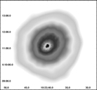
Figure 1: MOS1 image of ZW3146 in the [0.3-10] keV energy band. The image is corrected for vignetting and exposure and is adaptively smoothed (signal-to-noise ratio = 20).

We notice a sharp central surface brightness peak at a position $10^{\rm h}23^{\rm m}40^{\rm s}.01+04^{\circ}11^{\prime}09\hbox{$.\!\!^{\prime\prime}$}45$ (J2000), in very good agreement ($\Delta\alpha=0\hbox{$.\!\!^{\prime\prime}$}41$, $\Delta\delta=0\hbox{$.\!\!^{\prime\prime}$}55$) with the optical position of the central dominant cluster galaxy (Schwope et al., 2000). The morphology of the cluster is quite regular, thus indicating a relaxed dynamical state, even though we notice that the central core appears slightly shifted to the south-east with respect to the outer envelope, with a north-west to south-east elongation of the cluster core. The regular morphology of the cluster is indicative of a relaxed dynamical state, thus allowing us to derive a good mass estimate based on the usual assumptions of hydrostatic equilibrium and spherical symmetry (see Sect. 3.5).

3.2.1 Surface brightness profile

We computed a background-subtracted vignetting-corrected radial surface brightness profile in the [0.3-2] keV energy band for each camera separately. The profiles for the three detectors were then added into a single profile and binned such that at least a sigma-to-noise ratio of 3 was reached. The cluster emission is detected up to 1.5 Mpc ($\sim 6\arcmin$) and the profile appears relatively regular and relaxed (see Fig. 2).

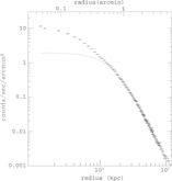
Figure 2: Background subtracted, azimuthally averaged radial surface brightness profile in the [0.3-2] keV range. The best fit $\beta$-model fitted over the 230 - 1300 kpc region (0$.\!\!^{\prime}$9-5$.\!\!^{\prime}$0) is over-plotted as a solid line. When extrapolated to the centre, this model shows a strong deficit as compared to the observed surface brightness.

The surface brightness profile of the undisturbed cluster was fitted with the CIAO tool Sherpa with various parametric models, which were convolved with the XMM-Newton PSF. The overall PSF was obtained by adding the PSF of each camera (Ghizzardi, 2001), estimated at an energy of 1.5 keV and weighted by the respective cluster count rate in the 0.3-2 keV energy band. A single $\beta$-model (Cavaliere & Fusco-Femiano, 1976) is not a good description of the entire profile: a fit to the outer regions (230$\;h_{70}^{-1}$ kpc $<r<$ 1300$\;h_{70}^{-1}$ kpc) shows a strong excess in the centre as compared to the model (see Fig. 2). The peaked emission is a strong indication for a cooling flow in this cluster. We found that for 230$\;h_{70}^{-1}$ kpc $<r<$ 1300$\;h_{70}^{-1}$ kpc the data can be described ($\chi^{2}_{\rm red}\sim 1.39$ for 74 d.o.f.) by a $\beta$-model with a core radius $r_{\rm c}=177\pm 2$$\;h_{70}^{-1}$ kpc and a slope parameter $\beta=0.77\pm 0.01$ (3 $\sigma$ confidence level). The single $\beta$-model functional form is a convenient representation of the gas density profile in the outer regions, which is used as a tracer for the potential. The parameters of this best fit are thus used in the following to estimate the total mass profile in the region where the single beta model holds (see Sect. 3.5).
We also considered a double isothermal $\beta$-model and found that it can account for the entire profile, if the very inner and outer regions are excluded: for 15 kpc$\;h_{70}^{-1}$ $<r<$ 1300$\;h_{70}^{-1}$ kpc the best fit parameters are $r_{\rm c1}=177\pm 2$$\;h_{70}^{-1}$ kpc, $r_{\rm c2}=39\pm 1$$\;h_{70}^{-1}$ kpc and $\beta=0.76\pm 0.01$ ($\chi^{2}_{\rm red}\sim 1.67$ for 95 d.o.f.). A common $\beta$ value is assumed in this model, but we also tried the fit with two different $\beta$ values, finding very similar results ($r_{\rm c1}=172\pm 2$$\;h_{70}^{-1}$ kpc, $r_{\rm c2}=45\pm 1$$\;h_{70}^{-1}$ kpc, $\beta_{1}=0.76\pm 0.01$ and $\beta_{2}=0.88\pm 0.01$; $\chi^{2}_{\rm red}\sim 1.68$ for 94 d.o.f.).

3.3 Temperature map

The temperature image of the cluster central region shown in Fig. 3 was built from X-ray colours. Specifically, we extracted mosaiced MOS images in four different energy bands (0.3-1.0 keV, 1.0-2.0 keV, 2.0-4.5 keV and 4.5-8 keV), subtracted the background and divided the resulting images by the exposure maps. A temperature in each pixel of the map was obtained by fitting values in each pixel of these images with a thermal plasma, fixing $n_{\rm H}$ to the Galactic value and the element abundance to 0.3 solar. In particular we note that the very central region is cooler than the surrounding medium and the north-west quadrant appears slightly hotter than the south-east one, even though no strong features are present.

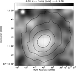
Figure 3: Temperature map obtained by using 4 X-ray colours (0.3-1.0, 1.0-2.0, 2.0-4.5, 4.5-8 keV) and estimating the expected count rate with XSPEC for a thermal MEKAL model, with fixed Galactic absorption $N_{H}$ and metallicity $Z$.

The regularity of the temperature distribution points to a relaxed dynamical state of the cluster, thus excluding the presence of an ongoing merger. Since cluster merging can cause strong deviations from the assumption of an equilibrium configuration, this allows us to derive a good estimate of the cluster mass (see Sect. 3.5).

3.4 Spectral analysis

Throughout the analysis, a single spectrum was extracted for each region of interest and was then regrouped to reach a significance level of at least 3 $\sigma$ in each bin. The data were modelled using the XSPEC code, version 11.3.0. Unless otherwise stated, the relative normalizations of the MOS and pn spectra were left free when fitted simultaneously. We used the following response matrices: m1_169_im_pall_v1.2.rmf (MOS1), m2_169_im_pall_v1.2.rmf (MOS2), epn_ff20_sY9.rmf (pn).

3.4.1 Global spectrum analysis

For each instrument, a global spectrum was extracted from all events lying within 5$\arcmin$ of the cluster emission peak. We tested in detail the consistency between the three cameras by fitting separately these spectra with an absorbed MEKAL model with the redshift fixed at z=0.291 and the absorbing fixed at the galactic value ($n_{\rm H}=3.01\times 10^{20}\mbox{ cm}^{-2}$, Dickey & Lockman, 1990). Fitting the data from all instruments above 0.3 keV led to inconsistent values for the temperature derived with the MOS and pn cameras: $kT=6.18^{+0.16}_{-0.15}$ keV (MOS1), $5.72^{+0.15}_{-0.14}$ (MOS2), $5.01^{+0.09}_{-0.08}$ (pn). We then performed a systematic study of the effect of imposing various high and low-energy cutoffs, for each instrument. Good agreement between the three cameras was found in the [1.0-10.0] keV energy range ($kT=6.27^{+0.21}_{-0.20}$ keV for MOS1, $5.99^{+0.20}_{-0.19}$ for MOS2, $6.00^{+0.16}_{-0.15}$ for pn). On the other hand, we also found consistent results by fitting the MOS spectra in the [0.4-10] keV energy range and the pn spectrum in the [0.9-10] keV energy range.The discrepancies observed by fitting the whole energy range are probably due to some residual calibration uncertainties in the low-energy response of all instruments. Thus, in order to avoid inaccurate measurements due to calibration problems, we adopted the low energy cut-off derived above for the spectral analysis discussed below.
The combined MOS+pn global temperature and luminosity are respectively $kT=5.91^{+0.09}_{-0.08}$ keV, $L_{X}\mbox{ (2-10 keV)}=2.0\pm 0.1\times 10^{45}\mbox{ erg s}^{-1}$ in the [0.4/0.9-10.0] keV energy range (MOS/pn) and $kT=6.08^{+0.11}_{-0.10}$ keV, $L_{X}\mbox{ (2-10 keV)}=2.0\pm 0.1\times 10^{45}\mbox{ erg s}^{-1}$ in the [1.0-10.0] keV energy range. These values are in agreement with ASCA results (Allen et al. 1996, Allen 2000), while Ettori et al. (2001) derived higher temperature values from BeppoSAX observations. The simultaneous fit in the [0.4/0.9-10.0] keV energy range (MOS/pn) to the three spectra is shown in Fig. 4.

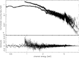
Figure 4: Global MOS (lower) and pn (upper) spectra in the [0.4/0.9-10.0] keV energy range (MOS/pn) integrated in a circular region of radius 5$\arcmin$. The fit with a MEKAL model and the residuals are shown.

3.4.2 Radial temperature profile

Table 1: Results from the spectral fitting in concentric annular regions in the [0.4/0.9-10.0] keV energy range (MOS/pn) and in the [1.0-10.0] keV energy range. Temperatures ($kT$) are in keV, metallicities ($Z$) in solar units and [2-10] keV luminosities ($L_{\rm X}$) in units of $10^{44}\mbox{ erg s}^{-1}$. The total $\chi^{2}$ values and numbers of degrees of freedom (dof) in the fits are also listed. Error bars are at the 90% confidence levels on a single parameter of interest.

		[0.4/0.9-10.0] keV energy range (MOS/pn)				[1.0-10.0] keV energy range
Radius	Radius (kpc)	$kT$	$Z$	$L_{\rm X}$	$\chi^{2}$/dof	$kT$	$Z$	$L_{\rm X}$	$\chi^{2}$/dof
0-20′′	0-87	$4.7^{+0.1}_{-0.1}$	$0.38^{+0.03}_{-0.03}$	5.68	1630/1503	$4.8^{+0.1}_{-0.1}$	$0.36^{+0.04}_{-0.03}$	5.77	1461/1403
20′′-40′′	87-174	$6.1^{+0.2}_{-0.2}$	$0.31^{+0.04}_{-0.04}$	5.15	1456/1421	$6.3^{+0.2}_{-0.2}$	$0.30^{+0.04}_{-0.04}$	5.20	1323/1321
40′′-1′	174-262	$6.7^{+0.3}_{-0.3}$	$0.25^{+0.05}_{-0.05}$	3.14	1145/1139	$6.9^{+0.3}_{-0.3}$	$0.25^{+0.05}_{-0.05}$	3.16	1040/1039
1′-1$.\!\!^{\prime}$5	262-393	$6.5^{+0.3}_{-0.3}$	$0.18^{+0.05}_{-0.05}$	2.41	1002/1007	$6.7^{+0.4}_{-0.3}$	$0.18^{+0.05}_{-0.05}$	2.43	892/907
1$.\!\!^{\prime}$5-2′	393-524	$6.7^{+0.5}_{-0.4}$	$0.28^{+0.08}_{-0.08}$	1.28	743/719	$7.0^{+0.6}_{-0.5}$	$0.28^{+0.08}_{-0.08}$	1.30	618/620
2′-3′	524-785	$7.0^{+0.6}_{-0.6}$	$0.24^{+0.10}_{-0.10}$	1.21	593/578	$7.4^{+0.8}_{-0.7}$	$0.22^{+0.10}_{-0.10}$	1.26	479/480
3′-5′	785-1309	$6.8^{+1.3}_{-0.9}$	$0.23^{+0.28}_{-0.22}$	0.79	306/253	$7.1^{+1.9}_{-1.2}$	$0.21^{+0.30}_{-0.21}$	0.80	241/195
0′-5′	0-1309	$5.9^{+0.1}_{-0.1}$	$0.30^{+0.02}_{-0.02}$	20.14	2632/1859	$6.1^{+0.1}_{-0.1}$	$0.28^{+0.02}_{-0.02}$	20.42	2399/1759

We produced a radial temperature profile by extracting spectra in annuli centred on the peak of the X–ray emission. The annular regions are detailed in Table 1. The data from the three cameras have been modelled simultaneously using a simple, single-temperature model (MEKAL plasma emission code in XSPEC) with the absorbing column density fixed at the nominal Galactic value. The free parameters in this model are the temperature $kT$, metallicity $Z$ (measured relative to the solar values, with the various elements assumed to be present in their solar ratios) and normalization (emission measure). We separately performed the spectral fitting in the [0.4/0.9-10.0] keV energy range (MOS/pn) and in the [1.0-10.0] keV energy range. The best-fitting parameter values and 90% confidence levels derived from the fits to the annular spectra are summarized in Table 1. The projected temperature profile determined with this model is shown in Fig. 5. We note that, as expected, temperature values derived in the [1.0-10.0] keV energy range are slightly higher than those derived in the [0.4/0.9-10.0] keV energy range (MOS/pn), even though consistent within the 90% confidence level. In the following discussion we adopt results derived in the [0.4/0.9-10.0] keV energy range (MOS/pn). The temperature rises from a mean value of $4.7\pm 0.1$ keV within 90$\;h_{70}^{-1}$ kpc to $kT=6.7\pm 0.5$ keV over the 180-1300 kpc region, where the cluster can be considered approximately isothermal. The lack of evidence for a temperature decline in the outer regions is in agreement with the results by Mushotzky (2003).

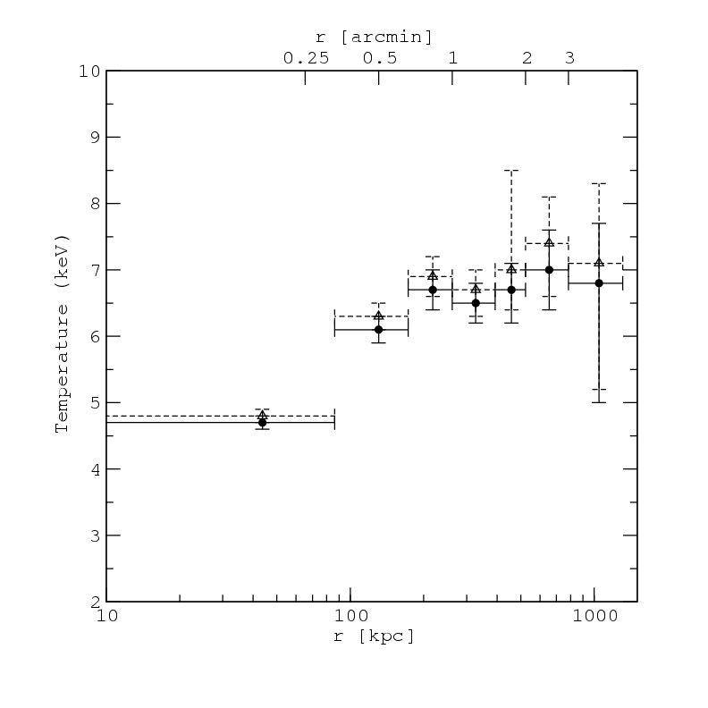
Figure 5: Full Circles: the projected X-ray gas temperature profile measured from XMM data in the [0.4/0.9-10.0] keV energy range (MOS/pn). Open Triangles: same as full circles, but in the [1.0-10.0] keV energy range.

The metallicity profile is shown in Fig. 6: a gradient is visible towards the central region, the metallicity increasing from $Z=0.18\pm 0.05$ over the 260-400$\;h_{70}^{-1}$ kpc region to $Z=0.38\pm 0.03$ inside the central 90$\;h_{70}^{-1}$ kpc.

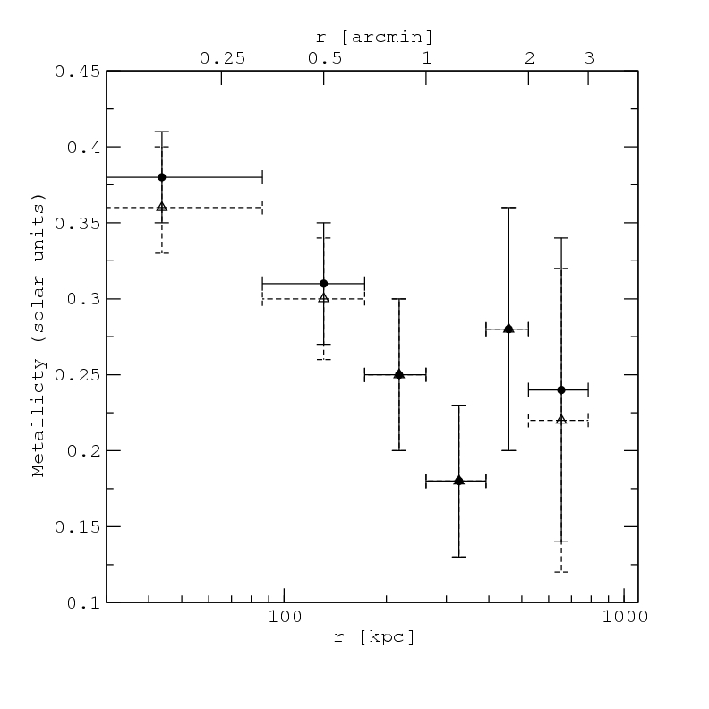
Figure 6: Full Circles: the projected X-ray gas metallicity profile measured from XMM data in the [0.4/0.9-10.0] keV energy range (MOS/pn). Open Triangles: same as full circles, but in the [1.0-10.0] keV energy range.

3.4.3 Cooling core analysis

The surface brightness profile, the temperature map and the temperature profile all give hints of the presence of a cooling core. Here we further investigate the physical properties of the ICM in the central region. The cooling time is calculated as the time taken for the gas to radiate its enthalpy per unit volume using the instantaneous cooling rate at any temperature:

$$t_{\rm cool}\approx\frac{H}{n_{\rm e}n_{\rm H}\Lambda(T)}=\frac{\gamma}{\gamma-1}\frac{kT}{\mu X_{\rm H}n_{\rm e}\Lambda(T)}$$ (1)

where $\gamma=5/3$ is the adiabatic index; $\mu\approx 0.61$ (for a fully-ionized plasma) is the molecular weight; $X_{\rm H}\approx 0.71$ is the hydrogen mass fraction; and $\Lambda(T)$ is the cooling function. We calculate the cooling function and the electron density by following the procedure described in Sect. 3.5, using the $\beta$-parameters derived by fitting the surface brightness profile over the 65 - 1300$\;h_{70}^{-1}$ kpc region (data in this region can be approximated by a $\beta$ model with $r_{\rm c}\sim 113$$\;h_{70}^{-1}$ kpc and a slope parameter $\beta\sim 0.70$). The cooling time is less than 10 Gyr inside a radius of 150$\;h_{70}^{-1}$ kpc ($\sim 0\hbox{$.\!\!^{\prime}$}6$), in agreement with the ROSAT result of Allen (2000).
We therefore accumulate the spectrum in the central $0\hbox{$.\!\!^{\prime}$}6$. We compare the MEKAL model already used in Sect. 3.4.1 and 3.4.2 with a model which includes a single temperature component plus an isobaric multi-phase component (MEKAL + MKCFLOW in XSPEC), where the minimum temperature, $kT_{\rm low}$, and the normalization of the multi-phase component, Norm${}_{\rm low}=\dot{M}$, are additional free parameters. The maximum temperature $kT$ of the MKCFLOW model is linked to the ambient value of the MEKAL model. This model differs from the standard cooling flow model as the minimum temperature is not set to zero.

Table 2: The best-fit parameter values and 90% confidence limits from the spectral analysis in the central $0\hbox{$.\!\!^{\prime}$}6$ region. Temperatures ($kT$) are in keV, metallicities ($Z$) as a fraction of the solar value and normalizations in units of $10^{-14}n_{\rm e}n_{\rm p}V/4\pi[D_{\rm A}(1+z)]^{2}$ as done in XSPEC (for the MKCFLOW model the normalization is parameterized in terms of the mass deposition rate $\dot{M}$, in $\mbox{M}_{\hbox{$\odot$}}\mbox{ yr}^{-1}$).

Parameter	MEKAL	MEKAL+MKCFLOW
$kT$	$5.2^{+0.1}_{-0.1}$	$8.6^{+1.1}_{-0.5}$
$Z$	$0.35^{+0.03}_{-0.02}$	$0.40^{+0.03}_{-0.03}$
Norm	6.67${}^{+0.07}_{-0.09}\times 10^{-3}$	1.07${}^{+0.48}_{-0.74}\times 10^{-3}$
$kT_{\rm low}$	—	$1.7^{+0.2}_{-0.2}$
Normlow	—	${\dot{M}}=1580^{+150}_{-130}$
$\chi^{2}$/dof	2024/1783	1903/1781

The results, summarized in Table 2, show that the statistical improvements obtained by introducing an additional emission component compared to the single-temperature model are significant at more than the 99% level according to the F-test, with the temperature of the hot gas being remarkably higher than that derived in the single-phase model. The fit with the modified cooling flow model sets tight constraints on the existence of a minimum temperature ($\sim$ 1.7 keV). We find a very high value of the nominal mass deposition rate in this empirical model: $\sim 1600\mbox{ M}_{\hbox{$\odot$}}\mbox{ yr}^{-1}$. ASCA-ROSAT observations already found a very strong cooling flow in this cluster (Allen 2000).

3.5 Mass determination

In the following we estimate the total mass of the cluster using the usual assumptions of hydrostatic equilibrium and spherical symmetry. Under these assumptions, the gravitational mass $M_{\rm tot}$ of a galaxy cluster can be written as:

$$M_{\rm tot}(<r)=-\frac{kT\,r}{G\mu m_{p}}\left[\frac{d\ln n_{g}}{d\ln r}+\frac{d\ln T}{d\ln r}\right]$$ (2)

where $G$ and $m_{p}$ are the gravitational constant and proton mass and $\mu\approx 0.61$. The deprojected $d\ln n_{g}/d\ln r$ was calculated from the parameters of the single $\beta$-model derived in Sect. 3.2.1. In particular, the advantage of using a $\beta$-model to parameterize the observed surface brightness is that gas density and total mass profiles can be recovered analytically and expressed by simple formulae:

$$n_{\rm gas}(r)=n_{\rm 0,gas}\left[1+\left(\frac{r}{r_{\rm c}}\right)^{2}\right]^{-3\beta/2}$$ (3)

$$M_{tot}(<r)=\frac{k\,r^{2}}{G\mu m_{p}}\left[\frac{3\beta rT}{r^{2}+r^{2}_{\rm c}}-\frac{dT}{dr}\right]$$ (4)

In estimating the temperature gradient from the profile shown in Fig. 5, only data beyond $30^{\prime\prime}$ ($\sim 130$$\;h_{70}^{-1}$ kpc) were considered: in the central bins the temperature as derived in Sect. 3.4.2 is more affected by the XMM PSF and projection effects, while for the outer regions these effects can be neglected (e.g. Kaastra et al., 2004). The total gravitating mass distribution derived from Eq. 4 is shown in Fig. 7 as a solid line, with errors coming from the temperature measurement and $\beta$-model represented as dashed lines. Within 1 Mpc we find a total mass of $\sim(5.4\pm 0.5)\times 10^{14}M_{\hbox{$\odot$}}$ and within the outer radius of the cluster as visible in the X-ray surface brightness profile (1.5 Mpc) we find $\sim(8.5\pm 0.7)\times 10^{14}M_{\hbox{$\odot$}}$. We note that the total integrated mass within a particular volume is dependent upon the local physical properties (temperature and density gradients) and is unaffected by the regions interior, or exterior, to that radius. The mass profile derived with this method is thus reliable in the region where the $\beta$-model is a good representation of the observed surface brightness profile (230 kpc $\lesssim$   r   $\lesssim$ 1300 kpc, see Sect. 2.3.1), whereas it cannot be extrapolated to the central region.
We also calculate the projected mass along the line-of-sight within a cylinder of projected radius $r$. The integration was performed out to a radius of $\sim 5$ Mpc from the cluster centre. The projected total mass is shown in Fig. 7 as a dashed-dotted line.

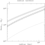
Figure 7: Solid line: Integrated total mass calculated from Eq. 4 (with error on the mass calculation coming from the temperature measurement and $\beta$-model shown by the dashed lines). Dashed-dotted line : Projected total mass with error. Dotted line: Gas mass.

In Fig. 7 we also show (dotted line) the gas mass profile derived by integrating the gas density given by Eq. 3 in spherical shells and using the $\beta$-model parameters determined in Sect. 3.2.1. The normalization of Eq. 3 is obtained from the combination of the best-fit results from the spectral and imaging analyses, which allows us to determine the conversion count rate - flux used to derive the bremsstrahlung emissivity that is then integrated along the line-of-sight and compared with the central surface brightness value. We note that, since we adopt the parameters of the $\beta$-model fit in the outer regions, the derived central electron density ($n_{\rm 0,e}\sim 1.7\times 10^{-2}\mbox{ cm}^{-3}$) is that predicted by the extrapolation of the $\beta$-model fit to the centre (see Fig. 2). This procedure is nonetheless reliable in estimating the gas mass for $r>230$$\;h_{70}^{-1}$ kpc, shown in Fig. 7.
In order to allow a direct comparison with our weak lensing studies in Sect. 5.1 and to derive an estimate of $r_{200}$ we perform a fit to the NFW profile (Navarro et al., 1996, 1997) given by

$$M_{\rm DM}(<r)=4\pi r^{3}_{\rm s}\rho_{\rm c}\frac{200}{3}\frac{c^{3}\left(\ln(1+r/r_{\rm s})-\frac{r/r_{\rm s}}{1+r/r_{\rm s}}\right)}{\ln(1+c)-c/(1+c)}$$ (5)

where $\rho_{\rm c}$ is the critical density. The scale radius $r_{\rm s}$ and the concentration parameter $c$ are the free parameters. The best fit parameters that minimize the $\chi^{2}$ of the comparison between the mass predicted by the integrated NFW dark matter profile and the mass profile reconstructed from Eq. 4 are: $r_{s}=516.6\pm 13$ kpc and $c=3.58\pm 0.07$, where the relation $r_{200}=c\times r_{s}$ holds. The quoted error are at the 68% confidence levels (1$\sigma$) on a single parameter of interest. Note that we neglect the gas mass contribution to the total mass and we assume $M_{\rm tot}(<r)=M_{\rm DM}(<r)$. We have also performed the same fitting procedure by including the gas mass, i.e. by assuming $M_{\rm tot}(<r)=M_{\rm DM}(<r)+M_{\rm gas}(<r)$, and find very similar results. In Fig. 27(a) we show confidence contours of the NFW fit to our mass profile and note that both parameters are well constrained. For a comparison to the equivalent model based on lensing data we refer to Sect. 7.

4 Optical observations

4.1 WFI-observations and data reduction

Z3146 was observed with WFI@ESO/MPG2.2m in the two observing programs 68.A-0255 (P.I. S. Schindler) and 073.A-0050 (P.I. P. Schneider). The first one obtained 8000s in broad band $V$ (BB#V/89_ESO843) and 16100s in broad band $R$ (ESO filter BB#Rc/162_ESO844). The second programme observed for another 8900s in $R$ and 1500s in $B$ (BB#B/123_ESO878). All data were processed with our image reduction pipeline developed within the GaBoDS project. It performs all necessary steps from raw frames to astrometrically and photometrically calibrated and co-added images. The individual methods and its performances on WFI data are described in detail in Schirmer et al. (2003) and Erben et al. (2005). All data were obtained during clear nights, under good seeing conditions ($\leq 1\hbox{$.\!\!^{\prime\prime}$}2$) and with a large dither box of about $3\hbox{$.\!\!^{\prime}$}0$ to ensure good flat-fielding and an accurate astrometric calibration. The images were tied to the astrometric frame of the USNO-A2 catalogue (Monet et al., 1998), photometrically calibrated with Stetson standards (Stetson, 2000) and finally co-added with the Swarp tool (Bertin, 2002). We produced several co-added images from our $R$ band exposures mainly to crosscheck our object shape measurements in the weak lensing analysis (see Sect. 5.1). The characteristics of all co-added images used in this work are summarised in Table 3 and Figs. 8 and 9. Each co-added science image has a pixel scale of $0\hbox{$.\!\!^{\prime\prime}$}238$ and is accompanied by a weight map characterising its noise properties.

Filter	Image Region	exp. time (s)	limiting magnitude ($3\sigma$ in a $2\hbox{$.\!\!^{\prime\prime}$}0$ aperture)	Seeing (arcsec)
$B$	(B)	1500	24.70	1.21
$V$	(I)	8040	25.02	1.16
$R$	(I)	16077	25.27	1.02
$R$	(B)	8850	25.24	1.11
$R$	(A)	24927	25.71	1.04

Table 3: Characteristics of the co-added WFI images. The limiting magnitudes quoted in column 4 are defined in the Vega system via $m_{\rm lim}=ZP-2.5\log(\sqrt{N_{\rm pix}}\cdot 3\cdot\sigma)$, where $ZP$ is the magnitude zeropoint, $N_{\rm pix}$ is the number of image pixels in a circle with radius $2\hbox{$.\!\!^{\prime\prime}$}0$ and $\sigma$ the sky background noise. The seeing in column 5 was measured with the SExtractor FWHM_IMAGE parameter. The groups in Bonn (B) and Innsbruck (I) observed Z3146 with an offset of about $5\hbox{$.\!\!^{\prime}$}0$ In Ra and $8\hbox{$.\!\!^{\prime}$}0$ in Dec. The exact layout is given in Fig. 8. For the $R$ band we created, besides the individual stacks, a deep mosaic in the common area (A). We note that the Innsbruck $R$ band has nearly double the exposure time of the Bonn image but about the same limiting magnitude as it was observed during less favourable moon phases. The quality of our photometric calibration is crosschecked in Fig. 9.

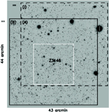
Figure 8: Layout of the Z3146 $R$-band WFI observations of the Bonn (B; solid lines) and Innsbruck (I; dashed lines) groups. The orientation with respect to the sky is North-Up and East-Left. The overlap in the $R$ exposures allows useful tests in the shape measurement procedures during our weak lensing analysis (see Sect. 5.1). If not stated otherwise we use the deep $R$ band stack from both observing campaigns and work in the common area (A) where we have data in $B$, $V$ and $R$ available. It has an extent of $25\hbox{$.\!\!^{\prime}$}8\times 23\hbox{$.\!\!^{\prime}$}8$ and the cluster is located $8\hbox{$.\!\!^{\prime}$}0$ north and $10\hbox{$.\!\!^{\prime}$}0$ west with respect to its lower left corner. The white square marks the $\sim 16\arcmin 40\arcsec\times 16\arcmin 40\arcsec$ region used in Sect. 5.2 and 6 for extracting the Red Sequence galaxies.

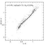
Figure 9: As a control check for our photometric calibration we plot colours of bright, unsaturated stars in our WFI fields compared to isochrones for stars of 10 Gyrs with a metallicity of 0.4% (see Girardi et al., 2002). Magnitudes for the stars were estimated with the SExtracor MAG_AUTO magnitude. Our data are in excellent agreement with the isochrone predictions.

4.2 HST-observations

In addition to our WFI observations we used archival calibrated HST data from the WFPC2 Associations obtained during a snapshot programme (PI: Edge, PID-number 8301). Z3146 was observed with the WFPC2 (filter F606W) in April 2000 for a total exposure time of 1000 s. The pixel scale is $\sim 0\hbox{$.\!\!^{\prime\prime}$}1$ per pixel, the seeing is measured with the FWHM_IMAGE keyword of SExtractor to be $\sim 0.1\arcsec$. The main purpose using these archival HST data was the identification and comparison of arc candidates with the ground based observations.

5 Lensing analysis

5.1 Weak lensing analysis

As a second method for determining the mass and its distribution of Z3146 we performed a weak lensing mass reconstruction. For a broad introduction on weak lensing and its application in cluster mass determinations see for instance Bartelmann & Schneider (2001). In the following we describe the creation of our background galaxy catalogue and the weak lensing analysis. Throughout the analysis we use standard weak lensing notation.

5.1.1 Lensing catalogue generation

We use the deepest image, the $R$-band for the weak lensing measurement. To create an object catalogue with shear estimates for all objects we first extract sources with the SExtractor (we use a detection threshold of 1.9 and a minimum area of 3 pixels for our detections) and the IMCAT softwares. While SExtractor produces a very clean object catalogue if the source extraction from the science images is supported by a weight map (see e.g. Fig. 27 of Erben et al., 2005), IMCAT calculates all quantities necessary to estimate object shapes. We merge the two catalogues and calculate shear estimates with the KSB algorithm (see Kaiser et al., 1995). For the exact application of the KSB formalism we closely follow the procedures given in Erben et al. (2001) with important modifications in the selection of stars that are used for the necessary PSF corrections (see Van Waerbeke et al., 2005). After the PSF corrections we reject all objects with an IMCAT significance $\nu<8$, a half light radius smaller or equal to that of bright stars, and a final modulus of the shear estimate $|e|>0.8$. In the following analysis we do not apply a weighting to individual galaxies.

Because of the large offsets between the observations from the Bonn and Innsbruck groups it is not obvious whether we can savely use the deep stack (A) for the lensing analysis or whether we have to work on the individual co-additions (I) and (B). This mainly comes from the assumption of a smooth variation of the PSF over the whole field-of-view when we correct galaxy shapes for PSF effects. With the large offsets we could suffer from discrete jumps in the PSF anisotropy within the (A) mosaic. However, in Fig. 10 we see that the PSFs of all three stacks are well behaved in the (A) area. We performed comparisons of the final shear estimates in the (I), (B) and (A) mosaics and found that they are in excellent agreement (see Figs. 11 and 12). Therefore we decided to use the (A) mosaic, which is the deepest image, for our primary analysis.

The next step is to clean our lensing catalogue from likely cluster members, foreground galaxies and faint stars. To this end we plot stars and bright galaxies ($R<22.0$), which have a high probability to be at a lower redshift than the cluster, in a colour-colour diagram (see Fig. 13). We note that all these objects mostly occupy a limited and well defined area in colour-colour space. We finally use the following criteria to clean our background source catalog: We reject all objects with $R<22.0$ and keep objects between $22.0<R<23.0$ if they do not lie in the following area of the $(B-V)$ vs. $(V-R)$ diagram: $-0.23<(V-R)-0.8(B-V)<+0.8;\;0.25<(V-R)<1.67;\;0.2<(B-V)<1.5$. We keep all objects with $R>23.0$ as probable background sources. We note that Clowe & Schneider (2002) and Dietrich et al. (2005) used similar criteria to identify foreground objects.

For our final lensing catalogue we additionally exclude all objects falling in masked image regions (around bright stars, satellite tracks etc.). This leaves us with about 12 galaxies per sq. arcmin as direct tracers of the cluster shear. Around the Brightest Cluster Galaxy (BCG) of Z3146, this average density is reached at a radius of about $45\hbox{$.\!\!^{\prime\prime}$}0$ with only very few sources in the cluster centre.

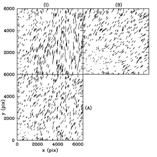
Figure 10: Stellar anisotropies for the fields (I), (B) and (A) in their common area.The length of the bars gives a measure for the stellar ellipticity and the direction the orientation of the semi-major axis. The longest bars correspond to an ellipticity of about $5\%$. All patterns show a smooth variation over the whole field-of-view of the (A) area.

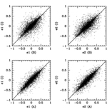
Figure 11: Galaxy ellipticities after all PSF corrections from completely independent analyses of the (I), (B) and (A) images in the overlap area. In the upper panels we compare the (B) and (I) sets which are independent (in terms of raw images entering the co-added stacks) from each other. The slopes of the fitted lines are 0.983 for e1 and 0.95 for e2. For the lower panels (comparison between (A) and (I)) the slopes are 0.992 for e1 and 0.974 for e2. The corresponding numbers for (A)-(B) are 1.080 for e1 and 1.091 for e2 (not shown in the figures). We conclude that the measurements are in very good agreement with each other. For the fits, the Ordinary Least Squares bisector method (see Isobe et al., 1990), which considers errors in e1 and e2, is chosen. After applying the line fits to the ellipticity components the mean shear differences are compatible with zero in all four cases. We note that the standard deviation of the residuals $\sigma_{\rm\Delta e}$ is 0.16 in both components for the (B)-(I) comparison but 0.10 in the (A)-(I) case. The cause for the lower value in the (A)-(I) case is that the data are not independent but share a large fraction of the input images. The residuals as function of position are discussed in Fig. 12.

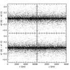
Figure 12: Differences of corrected galaxy ellipticity measurements from the (I) and (A) images as function of image position. We see no systematic trends of residuals with object position. Also a closer, visual inspection of the two-dimensional ellipticity residual distribution reveals no systematics on small scales. The standard deviation of the ellipticity components around zero is $\sigma_{\rm\Delta e}\approx 0.1$ in all four cases. Hence we conclude, together with the results of Fig. 11, that it is safe to use the (A) image for our weak lensing analysis.

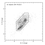
Figure 13: To obtain criteria to reject probable low $z$ foreground objects from our lensing analysis we plot all bright objects with $R<22.0$ in a colour-colour diagram. Most of them lie in a well defined area which we use to clean our catalogue. Elliptical cluster galaxies for a $z=0.3$ cluster are expected around $B-V\approx 1.2;\;V-R\approx 1.2$.

5.1.2 Weak lensing mass determination of Z3146

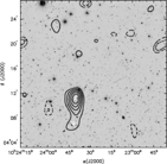
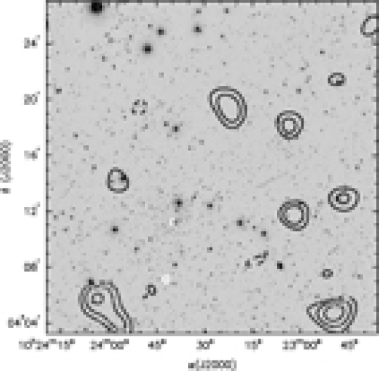
Figure 14: KS93 weak lensing cluster mass reconstruction of Z3146 (left panel). The shear field was smoothed with a Gaussian of width $1\hbox{$.\!\!^{\prime}$}4$. The $\kappa$ map was normalised so that the mean of $\kappa$ in the entire field is zero. Because we use this map only to define the centre of mass for model fits to the shear data the actual choice for this normalisation is not important. Solid contours increase in steps of $\Delta\kappa=0.01$ $(\sim 4.29\times 10^{13}M_{\odot}/$Mpc²), assuming a source galaxy redshift of 0.79. The cluster clearly shows up as the highest peak in this reconstruction. Dashed contours represent the same levels of negative $\kappa$. The white cross marks the cluster centre of our X-ray analysis (see Sect. 3.2) which is in excellent agreement with the lensing centre. The peak at the cluster position is detected with a significance of more than 4.1$\sigma$, the extension to the South (marked with a white circle) with $2.7\sigma$. Hence, this extension of the $\kappa$ map is not considered a significant lensing feature. The right panel shows a B-mode map of the $\kappa$ field. It contains two deeper holes in the southern part that are significant with $2.9\sigma$ (eastern hole) and $3.5\sigma$ (western hole). Around the cluster position this map shows a null signal. See the text for more details.

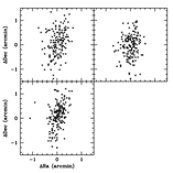
Figure 15: The lower left plot shows the lensing centres of our cluster reconstructions after adding noise realisations to our signal (see text for details). The quoted distances are with respect to the original cluster centre. Formal $1\sigma$ positional uncertainties of the lensing peak derived from this distribution are $\Delta R.A.=19\hbox{$.\!\!^{\prime\prime}$}8$ and $\Delta Dec=45\hbox{$.\!\!^{\prime\prime}$}6$. We investigated whether the observed asymmetry of the error distribution comes from shot noise in the galaxy ellipticities (the error might be dominated by a few very elliptical galaxies close to the cluster centre) or from the galaxy positions (as areas around bright stars or other image defects have been masked out the object distribution in our field is not homogeneous). To this end we assigned each galaxy a random ellipticity of a Gaussian distribution with $\sigma_{e}=0.38$ (see Sect. 5.1.2) and repeated our error analysis with 200 new noise realisations from this catalogue (upper left plot). For the upper right plot we additionally randomised the positions of our objects. Both simulations show a similar asymmetry as the original analysis and we conclude that it does not originate from shot noise of the galaxies. We note that the positional error estimates of this analysis are an upper limit as the original signal is already noisy (we implicitly assumed it to be noise free in our calculations).

The main interest of the weak lensing analysis in this work is an estimate of the total cluster mass of Z3146 and its inter-comparison with the X-ray analysis. We first perform a standard KS93 cluster mass reconstruction (see Kaiser & Squires, 1993) to investiagte the dark matter distribution and to obtain an estimate for the cluster centre. In addition, we calculate a B-mode map, i. e. we performed another mass reconstruction after all object ellipticities have been rotated by 45 degrees. This map should contain noise only if the lensing data are free from systematics. The results are discussed in Fig. 14. We see that our lensing centre is in excellent agreement with that determined from our X-ray analysis (see also Sect. 3.2) and we use the X-ray position for the following analysis. We estimate significances for peaks in our reconstructions and errors on the lensing centre with the following procedure: We randomise the orientation of our galaxies, redo a KS93 mass reconstruction with the new catalogue and repeat this procedure many times. For the peak significance we count how often the $\kappa$ value in our noise maps exceeds that of the lensing signal. With 29700 realisations the probabilities that the cluster peak, the cluster mass extension and the eastern and western holes in the B-mode map are pure noise features are 0/29700, 170/29700, 88/29700 and 9/29700. Assuming Gaussian statistics this translates to significances of $>4.1\sigma$, $2.7\sigma$, $2.9\sigma$ and $3.5\sigma$ respectively. We conclude that the highly significant cluster peak has no significant extension to the South. Next we estimate errors on the lensing peak position. The best way to measure the centroid dispersion would be to use a parametric model for the mass concentration and to generate noisy mass maps with randomised ellipticity orientations and galaxy positions. If the model were true we would obtain accurate error estimates from the noisy mass realisations. With the data at hand we can follow this idea by considering the original reconstruction as the input mass model. We probably overestimate the true error in this way because our input model already contains measurement noise. We plot the result of this exercise for 200 maps in the lower left panel of Fig. 15. We find a significant asymmetry in the distribution of positional differences. The positional accuracy is about 2.3 times better along R.A. than in Dec. As the mass distribution is elongated towards the South we would expect a skewed distribution of the positional errors towards negative Dec values but the observed symmetric elongation in the North-South direction is surprising. We checked that not a few, very elongated galaxies or shot noise from the galaxy positions (introduced for instance by object masks) are responsible for this result (see Fig. 15). Given this result we quote the positional accuracy of our lensing centre as $\Delta{\mbox{R}\rm a}=19\hbox{$.\!\!^{\prime\prime}$}8;\;\Delta{\mbox{D}\rm ec}=45\hbox{$.\!\!^{\prime\prime}$}6$.

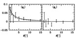
Figure 16: Left: Tangential shear signal as function of radius from the centre of Z3146. The signal is robust and we can trace the cluster shear up to the border of our data field. The solid line shows the reduced shear of our best fit NFW model $(r_{200}=1661\;h_{70}^{-1}\mbox{kpc},\,c=3.6)$, the dashed line that of an SIS fit ($\sigma_{v}=869$km/s). See the text for further details. Right: We show the cross component of the shear $g_{r}$ around the cluster centre, i. e. the signal after rotating all galaxies by 45 degrees. It should vanish if lensing caused the original signal and our measurement is compatible with zero over the entire distance range (see also Fig. 14). As a further consistency check we compare in Fig. 17 tangential shear measurements from the (I), (B) and (A) data sets.

While our mass maps give us insight into the dark matter distribution in Z3146 it is difficult to obtain reliable estimates for the total lensing mass and the involved errors. The main problems are that mass reconstructions involve a convolution from the measurable shear field and, in addition, they become very noisy at a distance several arcminutes from the cluster centre (see Fig. 14). Moreover, they intrinsically suffer from the mass-sheet degeneracy. Hence, we will estimate a lensing mass by directly fitting parametrised lensing models to the shear data. The error analysis is simplified significantly in this case. Moreover, model fits break the mass-sheet degeneracy by the explicit assumption that $\kappa$ at large distances from the lensing centre is zero. The main drawback is that shear data alone do not allow a clear discrimination between different, plausible mass models (see Fig. 16).

For our model fits to the shear data we primarily consider the universal density profile (NFW) proposed by Navarro et al. (1996). The details for the calculation of the lensing quantities $\kappa$ and $\gamma$ for this profile are given in several publications and the details are not repeated here (see e.g. Bartelmann, 1996; Kruse & Schneider, 1999). To determine our model parameters we use the log-likelihood method proposed in Schneider et al. (2000). We maximise the likelihood function:

$${\cal L}=\prod_{i=1}^{N}{1\over\pi\sigma^{2}[g(\theta_{i},a)]}\exp\left(-{|e_{i}+g(\theta_{i},a)|^{2}\over\sigma^{2}[g(\theta_{i},a)]}\right)\;,$$ (6)

where $N$ is the number of galaxies, $e$ the observed, two-dimensional ellipticity of each galaxy, $g$ the reduced shear of the model, $a$ the set of parameters to be fitted, $\theta$ the galaxy position in the lens plane and $\sigma$ the dispersion of the observed ellipticity. It is given by $\sigma=(1-|g|^{2})\sigma_{e_{\rm s}}$, where $\sigma_{e_{\rm s}}$ stands for the (two-dimensional) dispersion of the unlensed source ellipticities. All the model parameters $a$ are contained in $g$. The fundamental assumption of this method is that the source ellipticity distribution can well be described by a Gaussian distribution of width $\sigma_{e_{\rm s}}$. It is optimal in the sense that it uses the full ellipticity information and not only individual components (such as fits to the tangential part of the shear). For a more detailed discussion on this likelihood method and its properties see Schneider et al. (2000).

Before we apply this method we still have to specify the redshifts of the source galaxies and the galaxy sample we include in our fits. In Fig. 16 we show the tangential component of the shear around the cluster centre. We can trace the cluster shear signal over the whole field-of-view of $15\hbox{$.\!\!^{\prime}$}0$. Hence, we include all preselected background galaxies in our estimations. For the dispersion of the unlensed ellipticities $\sigma_{e_{\rm s}}$ we use the measured value of our galaxies $\sigma_{e}$ averaged over the whole field-of-view. Here we assume that weak lensing does not change this value significantly and we estimate $\sigma_{e_{\rm s}}=0.38$. For the redshift distribution of our background galaxies we use estimates from Hetterscheidt et al. (2006). The authors obtained photometric redshifts for 62000 galaxies with $21.5<R<24.5$. Their WFI data consist of 1.75 sq. degree of deep $UBVRI$ photometry in three different patches (see Hetterscheidt et al., 2006; Hildebrandt et al., 2006, for details on the data). The photometric redshift distribution is parametrised by the following function introduced by Brodwin et al. (2006):

$$p_{\rm fit}(z)=A\,\left[p_{1}(z)\,H(z_{\rm t}-z)+p_{2}(z)\,H(z-z_{\rm t})\right],$$ (7)

where $H$ denotes the Heaviside step function,

$$p_{1}(z)=\left(\frac{z}{z_{0}}\right)^{\alpha}\exp\left[-\left(\frac{z}{z_{0}}\right)^{\beta}\right]$$ (8)

and

$$p_{2}(z)=\exp{\left[\left(\frac{z_{t}}{z_{1}}\right)^{\gamma}-\left(\frac{z}{z_{1}}\right)^{\gamma}\right]}\,p_{1}(z_{\rm t});$$ (9)

the normalisation $A$ is obtained by

$$\int_{0}^{z_{\rm t}}{\rm{d}}z\,p_{1}(z)+\int_{z_{\rm t}}^{\infty}{\rm{d}}z\,p_{2}(z)=1.$$ (10)

For $z_{\rm t}=1$ the reported fit parameters are: $z_{0}=0.27$, $\alpha=2.84$, $\beta=1.40$, $\gamma=2.34$ and $z_{1}=2.16$. With this choice the mean redshift for galaxies behind our cluster at $z_{\rm cl}=0.29$ is $\langle z_{\rm bg}\rangle=0.79$. We use this distribution to estimate the average geometrical lensing factor:

$$D_{\rm d}(z_{\rm cl})\left\langle\frac{D_{\rm ds}(z_{\rm cl},z)}{D_{\rm s}(z)}\right\rangle=D_{\rm d}(z_{\rm cl})\int_{z_{\rm cl}=0.29}^{\infty}{\rm{d}}z\,p_{\rm fit}(z)\frac{D_{\rm ds}(z_{\rm cl},z)}{D_{\rm s}(z)},$$ (11)

where $D_{\rm d}$, $D_{\rm ds}$ and $D_{\rm s}$ represent angular diameter distances observer-cluster, cluster-background source and observer-background source respectively.

For our fits to the NFW profile, we consider the concentration $c$ and the radius $r_{200}$ (see Navarro et al., 1996) as free model parameters. With our setup, the application of our prescription to the shear data leads to best fit values of $r_{200}=1661^{+280}_{-328}\;h_{70}^{-1}$kpc and $c=3.6^{+2.8}_{-2.4}$. The model has a significance of 4.35 over one with zero mass and the errors on $r_{200}$ and $c$ are at the $90\%$ confidence level. They were estimated with our likelihood analysis by keeping $c$ or $r_{200}$ at its best fit value and leaving $r_{200}$ or $c$ as the only free parameter. In Fig. 27(b) we show confidence contours of our analysis and note that both parameters are reasonably well constrained except for low values of $c$ see Sect. 7 for a comparison to an NFW model based on X-ray data). In addition to the NFW profile we also modeled our shear data by a Singular Isothermal Sphere (SIS) characterised by its velocity dispersion $\sigma_{v}$. Our best fit model has $\sigma_{v}=869^{+124}_{-153}$km/s. The errors represent the 90% confidence level and the model has a significance of $4.88\sigma$ compared to the zero mass model. In contrast to the NFW fit, the significance and the estimated velocity dispersion of the SIS model show some dependence on the galaxies included close to the cluster centre. We notice an increase of significance by excluding the galaxies in a circle $30\hbox{$.\!\!^{\prime\prime}$}0$ around the cluster (five objects) and a smooth decrease of $S/N$ if we reject more galaxies beyond that point. Hence, we used all galaxies with a distance greater than $30\hbox{$.\!\!^{\prime\prime}$}0$ from the cluster centre for our SIS fit.

We finally discuss a possible bias of our result due to a systematic underestimate of the shear. As we showed in Erben et al. (2001) and within the Shear Testing Program (see Heymans et al., 2005) our pipeline may underestimate weak shear by 10%-15%. We recalculated the best fit NFW values after boosting all ellipticities by a factor of 1.15. We then obtain $r_{200}=1701^{+261}_{-303}\;h_{70}^{-1}$kpc and $c=3.66^{+2.52}_{-2.18}$ which is well within the error bars of the original signal. Hence, a possible systematic underestimate of the shear by about 15% would not change our results significantly. At the end of this section we show in Fig. 18 the total mass properties given by our model fits. We also present a mass-to-light ratio analysis in Sect. 6.3 and will compare our results with masses from X-ray analyses in Sect.7.

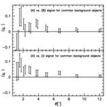
Figure 17: The figure shows comparisons of the tangential shear signal around Z3146 from common background objects for the (A) and (B) (upper panel) and the (A) and (I) sets (lower panel). The left measurements are from (A) and the shifted ones from (B) and (I) respectively. The catalogues of common sources were created by merging our lensing objects from (A) with the ellipticity catalogues from (I) and (B); see Fig. 11. As in the ellipticity comparisons, the tangential shear signals around the cluster agree reasonably well. A very different behaviour is observed for the first bin to which only about a dozen galaxies contribute. Note that the initial catalogues were created independently and hence the object samples in the two comparisons are not exactly the same.

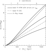
Figure 18: Total weak lensing mass calculated from our best fit mass models in spheres of radius $r$ around the cluster centre. Solid lines encompass our best fit NFW model $r_{200}=1661^{+280}_{-328}\;h_{70}^{-1}$kpc; $c=3.6$ with the errors from the measurement in $r_{200}$. With this model our total mass at $r_{200}$ is $M_{200}=7.05^{+2.8}_{-2.72}\times 10^{14}M_{\odot}$. The long-dashed curve represents our best SIS fit to the shear data. The mass at $r_{200}$ is 17% lower in this case. The total X-Ray mass of Z3146 (see Sect. 3.5) is given by the short-dashed line. It is $M_{200}=9.57^{1}0{14}M_{\odot}$.

5.2 Strong lensing analysis

5.2.1 Definition/identification of gravitational arc candidates

In addition to the weak lensing analysis we have searched the central cluster region for strongly lensed objects. In ground based observations usually only arcs tangentially aligned with respect to the mass centre are visible, as radial arcs are very thin and faint structures in the vicinity of bright central galaxies of clusters. In addition, arcs and their counter images have the same spectra and redshifts $\gtrsim 2\times z_{\rm lens}$. However we do not have spectra, hence apart from the position and the morphology, the redshift is the main identification criterion. Therefore we investigated whether it is possible using our observations to roughly estimate the photometric redshift or at least to find out whether an object belongs to a fore- or background population. For that purpose we have performed simulations using the software package hyperz (Bolzonella et al., 2000). We created a set of 3000 artificial galaxies with the following parameters: $0\leq z_{sim}\leq 2$, $R$ magnitude $22\leq m_{R}\leq 25$ (which corresponds to the range of the arc candidates), using the simulated filter WFI $R$ band (ESO844) as the reference filter. The type of the galaxies was also randomly chosen to be either E, S0, Sa, Sb, Sc or Sd. The simulations have shown that it is not possible to obtain any reliable redshift estimate from $BVR$ images only. 38% of all simulated galaxies with $z\leq z_{Z3146}$ were found to be background objects. On the other hand, 27% of the background galaxies (defined as $z\geq z_{Z3146}$) were measured to be located in front of Z3146. Hence it is even not possible to decide whether an object of unknown redshift is a foreground or a background object and we have to restrict our search for strongly lensed objects to morphological criteria only.
Unfortunately there is no common definition of an arc candidate. The definition we adopt of a gravitational arc candidate is that of an elongated object, aligned tangentially with respect to the cluster center, a minimum length of 1$.\!\!^{\prime\prime}$0 and a length-to-width ratio $l/w\geq 1.5$. However it is not yet clear whether Z3146 can produce strong lensing or not: the low concentration parameters $c$ obtained during the modelling of both, the X-ray ($c=3.58\pm 0.07$, $r_{200}=1849\pm 47\;h_{70}^{-1}$kpc, see Sect. 3.5) and the weak lensing data ($c=3.6^{+2.8}_{-2.4}$, $r_{200}=1661^{+280}_{-328}\;h_{70}^{-1}$kpc, see Sect. 5.1.2) to an NFW profile, leads to an Einstein ring of only $\sim 1\arcsec$. However, due to the large errors in both the $c$ and $r_{200}$ determination and the unknown source redshift, we cannot exclude the strong lensing ability: a source redshift of $z=2$ and adopting the upper limits of $c$ and $r_{200}$ (leading to $c=6.4$ and $r_{200}=1941\;h_{70}^{-1}$kpc, based on weak lensing values) shifts the Einstein ring to $\sim 13\arcsec$. Additionally, our adopted SIS model derived in Sect. 5.1.2 leads to an Einstein radius of the same size, assuming the source located at the derived mean redshift $\langle z_{\rm source}\rangle=0.79$. Adopting $\sigma_{v}=993$ km/s, the upper limit, leads to a critical curve at $\sim 22\arcsec$. Hence we restrict our search to regions within a radius of about $30\arcsec$, centred on the position of the Bright Central Galaxy.
In a deep arc search using the WFPC2 archive, Sand et al. (2005) quote one arc in this archival HST data set (A1 in our data set). Our identification of strong lensing features was done by visual inspection of the WFPC2 frames in direct comparison with the deep WFI exposures. As some of the candidates are very similar to not fully removed cosmics we carefully searched for all identified objects whether there is a corresponding object on all WFI frames. In this way we identified 4 objects in total (denoted as A1,...,A4) in the chosen field as good candidates for being strong lensing features (see Figs. 19 and 20).
A comparison even with shallow space based observations is a good method to identify possible gravitational arcs due to the missing atmospheric blurring effects. Several of the arc candidates were smoothed on the WFI images so as to even lose their tangential alignment. In particular, objects A3 and A4 are so strongly influenced by observational effects that they are not identifyable as arcs in ground based observations. A detailed comparison between the WFI and WFPC2 images of the arcs is shown in Fig. 20. Note that the exposure time of the WFI $R$-image is  6.9 h, whereas for the WFPC2 it was only $\sim$0.28 h. Nevertheless, the arc candidates visible in the HST image are clearly recognizable as possible gravitational arcs, whereas in the WFI frame seeing effects dominate the shape of the objects.

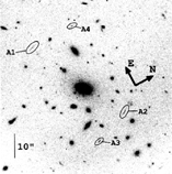
Figure 19: HST image of Z3146 obtained by the WFPC2. The exposure time was 1000 s using the filter F606W. The objects A3 and A4 were found on the HST frame by visual inspection (see Sect. 5.2.1 for more details).

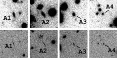
Figure 20: Detailed comparison of the arc candidates in Z3146 (top: WFI, bottom: WFPC2). In all images North is up, East to the left, the FoV is $15\arcsec\times 15\arcsec$. See text for more details.

5.2.2 Determination of the length-to-width ratio

To measure the length-to-width ratio $l/w$ we used SExtractor to detect the arc candidates on the WFPC2 image as it is not affected by atmospheric blurring. Due to its shallowness we used a value of 0.75 for DETECT_THRESH and ANALYSIS_THRESH. The $l/w$ ratio itself was determined using the same ansatz as in Lenzen et al. (2004) and Bertin (2005): we treat the arcs as a set of pixels with a certain light intensity value at each pixel. The light distribution of a certain object is then defined by all corresponding pixels detected by SExtractor shown in the SEGMENTATION images. Hence we can compute the second moments $\lambda_{1}$ and $\lambda_{2}$ of this light distribution in the usual way (see e.g. Lenzen et al., 2004; Bertin, 2005). Although the length $l$ is not equal to $\lambda_{1}$ and the width $w$ is not equal to $\lambda_{2}$ the ratio $l/w$ is equal to $\lambda_{1}/\lambda_{2}$ (Jähne, 2002). Hence we obtain the length-to-width ratio by determining $\lambda_{1}$ and $\lambda_{2}$.

5.2.3 Photometry / catalogue creation

The photometry was also performed with the software package SExtractor 2.3.2. In contrast to the determination of $l/w$ we used the WFI frames for this purpose, as those images are much deeper (see Table 3). The photometric measurement on the WFPC2 image was skipped as the F606W filter is fully covered by the $V$ and $R$ band of the WFI observations.
As we concentrate on the cluster itself we restricted the extraction of object catalogues to a FoV of $\sim\leavevmode\nobreak\ 16\arcmin 40\arcsec\times\leavevmode\nobreak\ 16\arcmin 40\arcsec$ (4.26$\;h_{70}^{-1}$ Mpc $\times$ 4.26$\;h_{70}^{-1}$ Mpc in our cosmology). The $V$ and $R$ images were convolved with a slight Gaussian filter of width 0.61 and 0.91 pixels, respectively, to bring all observations to the same seeing of $\sim 1\hbox{$.\!\!^{\prime\prime}$}2$ ($\Delta FWHM\leq 10^{-3}$″) and hence ensure that all objects are measured with the same photometric apertures.
We used SExtractor in double image mode with the deep $R$ band image as detection frame and the following parameters: DETECT_THRESH=7, ANALYSIS_THRESH=7, and DETECT_MINAREA=3 (the higher detection threshold compared to the weak lensing analysis is a result of the seeing correction). All magnitudes are obtained using MAG_AUTO with PHOT_AUTOPARAMS=1,3.5, as elliptical apertures and a Kron radius of this size is best suited to our observations. In order to obtain clean catalogues with a minor fraction of defective detections like obvious stars/foreground galaxies, traces of asteroids and spurious detections in bright haloes of stars we masked such objects to remove them from the final catalogues. The image of Fig. 21 shows as example the original $R$-band image including all masked objects within a FoV of $\sim\leavevmode\nobreak\ 16\arcmin 40\arcsec\times\leavevmode\nobreak\ 16\arcmin 40\arcsec$ (4.26$\;h_{70}^{-1}$ Mpc $\times$ 4.26$\;h_{70}^{-1}$ Mpc in our cosmology). All masks were identical for the final $B$ and $V$ image, except for the individual satellite tracks.
The total galaxy catalogue contains 2138 objects having a CLASS_STAR parameter $<$ 0.95, MAG_AUTO$<$99 in all bands (considering an $E(B-V)=0.126$ mag, taken from the NED, based on Schlegel et al. (1998)) and a FLUX_RADIUS $>3.2$ pixels in $B$, $V$ and $R$, respectively. In addition we used WEIGHT maps created by the data reduction pipeline (see Erben et al., 2005; Erben & Schirmer, 2003, for more details).

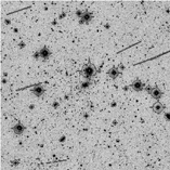
Figure 21: $R$-band image of Z3146. The image has a FoV of $\sim\leavevmode\nobreak\ 16\arcmin 40\arcsec\times\leavevmode\nobreak\ 16\arcmin 40\arcsec$ (4.26$\;h_{70}^{-1}$ Mpc$\times$4.26$\;h_{70}^{-1}$ Mpc), the lines are the masks which were used to remove satellite tracks, foreground galaxies and bright halos from stars (see text for more details). North is up, East to the left.

5.2.4 Analysis of the strong lensing features

The results of the photometric and morphological investigations of all 4 arc candidates are summarised in Table 4 and Table 5, respectively. In this section we analyse the arc candidates using these informations.
We can roughly estimate the strong lensing mass inside an Einstein ring at the position of the outer most arc A1 ($\sim 27\arcsec\sim 120$ kpc). This mass can be estimated to be $M_{\rm sl}=1.39^{+0.36}_{-0.35}\times 10^{14}M_{\odot}$, where the main value is derived for $\langle z_{\rm source}\rangle=0.79$, the mean redshift value obtained in Sect. 5.1.2. The errors are calculated for $z_{\rm source}=[2\times z_{\rm Z3146},2]$. However, as we do not know either the redshift or the geometric alignment of the source with respect to the lens, this procedure gives only a rough upper limit of the mass in the core.
One of the most interesting questions is the possibility of finding multiple images of one single background source. Unfortunately we do not have spectra of the objects (see Sect. 5.2.1) which allow a secure identification of counter images. Hence we search for counter images in the following way:
Counter images of arcs may not appear as elongated objects in the case of a folded arc system. In addition, they can differ in magnitudes due to the gravitational magnifying effect and can appear in unexpected locations (Broadhurst et al., 2005a), which are not predictable without a precise model. Hence we have to restrict the identification of multiple lensed objects to investigations of the colour information ($B-V$), ($B-R$), and ($V-R$) only, as they are conserved by lensing.
The search for multiple images was performed for all 4 arc candidates independently in 2 steps: first, we searched the galaxy catalogue for objects with (a) coinciding colours $(V-R)$, $(B-R)$ and $(B-V)$, and (b) lying in a radius of 30$.\!\!^{\prime\prime}$0 with respect to the cluster center position in the RBS. In a second step we discarded all objects being obvious cluster or foreground galaxies by visual inspection.
arc candidate A1: In total we found two objects which might be counter images of candidate A1, denoted by C1, and C2, respectively (see Fig. 23). It is hard to judge whether those objects are counter images as they are hardly visible in the shallow WFPC2 image. However, C2 is located at a distance of $\sim 30\arcsec$ with respect to the cluster center and hence we expect it to be much more sheared at this position if it had originated from the same object as A1. Additionally, the colours agree only within their large error bars (see Table 5 for the numbers). Hence we conclude that it is quite unlikely that this object is a counter image of A1.
arc candidates A2 and A3: Both candidates show colour coincidences with each other and C1 - C3. However, again the colour differences only agree within their error bars (see Table 5 for the numbers). The colour of A2 might be reddened to a certain amount by elliptical galaxies in its vicinity, nevertheless it is very unlikely that these objects have the same source.
arc candidate A4: We did not find any counter image candidates for this object.
Counter images also often occur nearby the central galaxy in the case of a not perfect alignment between the observer, the lens and the source. Hence they lie in the halo of a bright central object affecting their colour and/or are dramatically sheared up to a radial arc (see Sand et al., 2005, for some examples). Therefore we investigated the BCG using the HST image in more detail.
A closer look at the WFPC2 exposure of the BCG reveals some knots in its very central part. To investigate these structures and to look for a possible radial arc we subtracted as a first step an elliptical model derived by fitting ellipses to isophotes of the BCG (done with the help of the IRAF tasks isophote and bmodel in the STSDAS package) as well as an artificial de Vaucouleur profile (task mkobjects in noao.artdata).
Fig. 22 shows the central part of Z3146 with and without the subtracted elliptical isophote model of the BCG. The removal of the BCG reveals, apart from several clumps, an elongated substructure in the centre of the BCG along its major axis in the opposite direction to A1. However, we need deeper observations for identification of this object. At the current stage we can neither exclude the possibility of this object of being a radial arc or a filamentary structure common in cooling flow clusters.

However, the fact that we did not find definitive counter images in our observations does not mean that there are none. Lensed sources can appear as very faint and thin arclets which are only visible in deep HST observations. Such arclets are therefore hard to find in ground based observations. Some prominent examples of lensing clusters such a large number of faint arc(lets) are e.g. A2218 (see Soucail et al., 2004, and references therein), A1689 (Broadhurst et al., 2005a), A370 (Bézecourt et al., 1999) or CL0024+16 (Broadhurst et al., 2000; Kneib et al., 2003).

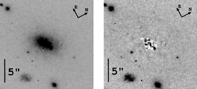
Figure 22: HST image of the innermost part of Z3146. In the right image we subtracted an elliptical model (based on fitting an ellipse to each isophote obtained by the IRAF tasks isophote and bmodel in the STSDAS package). Several distinct substructures are visible, but require deeper observations for their identification.

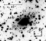
Figure 23: $R$-band image taken with WFI. Possible counter images of the arc candidates are denoted with Cx. See Sect. 5.2.4 for the relations of the Cx to the arc candidates.

arc candidate	angular distance	projected dist.	length $l$	$l/w$	filter
in Fig.19	to cc	to cc [kpc]	[ $\arcsec$ ]	WFPC2	$B$ [mag]	$V$ [mag]	$R$ [mag]
A1	$\sim 27$	$\sim 117$	2$.\!\!^{\prime\prime}$3	$5.1$	$24.49\pm 0.28$	$23.87\pm 0.06$	$22.73\pm 0.01$
A2	$\sim 20$	$\sim 87$	2$.\!\!^{\prime\prime}$0	$5.6$	$23.89\pm 0.22$	$23.07\pm 0.04$	$22.06\pm 0.01$
A3	$\sim 23$	$\sim 100$	1$.\!\!^{\prime\prime}$4	$2.1$	$24.20\pm 0.21$	$23.68\pm 0.05$	$22.71\pm 0.01$
A4	$\sim 26$	$\sim 113$	1$.\!\!^{\prime\prime}$1	$1.9$	$24.64\pm 0.22$	$24.08\pm 0.05$	$23.64\pm 0.02$

Table 4: Table of the arc candidates shown in Fig.19. ’cc’ denotes the cluster centre, the length-to-width ratio $l/w$ is calculated with the help of $\lambda_{1}$, and $\lambda_{2}$ (the second order moments of the light distribution) and is measured on the WFPC2 images as it is not affected by atmospheric blurring. A value of $=0.75$ was chosen for both, the DETECT_THRESH and ANALYSIS_THRESH due to the shallowness of the image. The magnitudes are instrumental WFI magnitudes in the Vega system. All objects are photometrised using SExtractor’s MAG_AUTO.

object	$(V-R)$	$\Delta(V-R)$	$(B-R)$	$\Delta(B-R)$	$(B-V)$	$\Delta(B-V)$
A1	1.14	0.07	1.76	0.29	0.62	0.34
A2	1.01	0.05	1.83	0.23	0.82	0.26
A3	0.97	0.06	1.50	0.22	0.52	0.26
A4	0.44	0.07	1.00	0.24	0.55	0.27
C1	1.15	0.12	2.37	0.79	1.22	0.87
C2	1.02	0.1	2.26	0.74	1.24	0.81
C3	0.89	0.1	2.74	1.06	1.85	1.12

Table 5: Photometric properties of the arc candidates and their possible counter images. See Sect. 5.2.4 for more details and discussions.

6 Investigations of the cluster light distribution

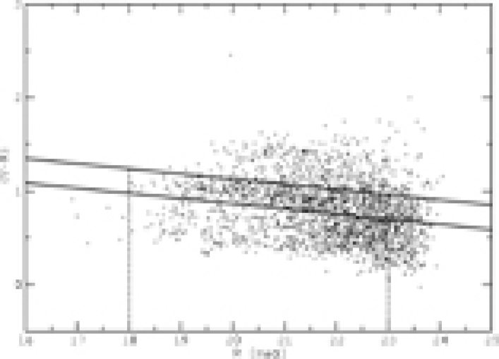
Figure 24: $(V-R)$ vs. $R$ colour-magnitude diagram. A distinct Red Sequence is visible, framed by two solid lines. The dashed lines show the limits used for identification of cluster members (see text for more details).

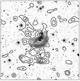
Figure 25: Galaxy density plot of Z3146. The FOV ($\sim 16\arcmin 40\arcsec\times 16\arcmin 40\arcsec$) is centred on the BCG, north is up, east to the left, $1\hbox{$.\!\!^{\prime\prime}$}0=4.36\;h_{70}^{-1}\,$kpc. The image shows the distribution of the main Red Sequence galaxies shown in the upper plot of Fig.24. The contour levels correspond to $0.6,0.8,1,...,2.4\times 10^{-4}$ galaxies/arcsec². (The small dip in the contours between the cluster center and the bright star in the north is most likely an artifact from the masked and hence removed parts of the image, see Fig. 21)

In this section we present additional optical investigations on Z314 6 which are based on the WFI frames.

6.1 Cluster member catalogue

Independent of the previous analyses we have created different catalogues as we have different selection criteria for the further investigations. The lensing analysis focuses on background objects, whereas the following investigations deal with the cluster members. We extracted a catalogue of cluster members in the following way:
(a) From the galaxy catalogue created in Sect. 5.2.3 we made the colour-magnitude diagram $(V-R)$ vs. $R$ (see Fig. 24). In this plot we identify a Red Sequence (henceforth RS, marked by the two solid lines) which is used as the basis for the cluster member detection. The extraction of the Red Sequence was done by eye. As the RS galaxies belong to the ellipticals, which are the reddest ones in a galaxy cluster, we use the upper limit of the RS distribution as the natural colour border and assume all objects below the upper RS limit as cluster members. Additionally we skipped all objects with $R\geq 23.5$ mag as likely belonging to a background population, and objects with $R\leq 18$ mag as likely foreground systems. With these criteria we found in total 756 RS galaxies and 1478 cluster members.

6.2 Galaxy distribution in Z3146

To investigate the distribution of the RS members we created galaxy density maps in the following way: a blank image of about $4200\times 4200$ pixels (corresponding to a FoV of $\sim\leavevmode\nobreak\ 16\arcmin 40\arcsec\times\leavevmode\nobreak\ 16\arcmin 40\arcsec$, 4.26$\;h_{70}^{-1}$ Mpc $\times$ 4.26$\;h_{70}^{-1}$ Mpc) was created with pixel value ”0” everywhere. At each position of the extracted Red Sequence galaxies (see Sect. 5) the pixel value was changed to ”1” and a subsequent Gaussian smoothing with $\sigma=241$ pixels (corresponds to 250$\;h_{70}^{-1}$ kpc) leads to the image in Fig.25.
The galaxy density plot of the main Red Sequence (Fig.25) shows one large peak centred on the main cluster with no distinct subclumps, except one small peak south of the cluster core. This is an indication that Z3146 is a relaxed cluster without any ongoing major merger event, which is confirmed by the massive cooling flow found in previous investigations (Edge et al., 1994; Fabian et al., 2002) and our own results of $\sim 1600$ M_⊙ per year. In particular, the small distance of about $0\hbox{$.\!\!^{\prime\prime}$}69$ between the optical and the X-ray centre (Schwope et al., 2000) also confirms the calm character of this cluster.

6.3 Light distribution / mass-to-light ratio

In order to obtain a mass-to-light ratio and creating a light distribution map we applied the K-correction as a first step. We used the MatLab^© script lum_func.m written by Eran Ofek for this purpose. As input parameters we used the corresponding WFI filter curves and template spectra provided by Stephen Gwyn which are based on spectra by Coleman et al. (1980). As Red Sequence galaxies are mainly ellipticals we used E/S0 spectra for them and Sbc templates for the remaining. The resulting K-corrections (see Table 6) were applied to the galaxy catalogues of all galaxies in the FoV. To take the contamination resulting from non-cluster members into account we created another catalogue of galaxies with the same criteria from a different region on the final WFI frames. This field is centered on $\alpha=10^{\rm h}22^{\rm m}59^{\rm s}$ and $\delta=+04^{\circ}20\arcmin 33.3\arcsec$, has the same size as the region used for creating the cluster member catalogue and has no distinct galaxy density peak. Hence we assume the galaxy population in this field to be dominated by field galaxies. Additionally this region is, in spite of the pointing offset between the different observing programs (see Sect. 4), visible on all three observed bands. The galaxy counts in this field were binned in the same way as in the cluster field and subtracted from the corresponding bin of the cluster count.

	$B$	$V$	$R$	units
E/S0 K-correction	1.41	0.85	0.32	[mag]
Sbc K-correction	0.84	0.33	0.14	[mag]
fitting range $M_{fit}$	$<-19$	$<-19$	$<-19$	[mag]
$\phi^{*}$	$1.814^{+2.24}_{-2.24}\times 10^{3}$	$0.8^{+2.81}_{-2.81}\times 10^{3}$	$0.907^{+1.121}_{-1.121}\times 10^{3}$	[# galaxies deg-2]
$\alpha$	$-1.136^{+0.53}_{-0.53}$	$-1.38^{+1.30}_{-1.30}$	$-1.24^{+0.33}_{-0.33}$
$M^{*}$	$-20.6^{+1.3}_{-1.3}$	$-21.74^{+3.01}_{-3.01}$	$-22.53^{+1.55}_{-1.55}$	[mag]
$\chi^{2}$	0.972	0.952	0.973
$L_{tot}$	$1.12\times 10^{14}$	$0.98\times 10^{14}$	$1.38\times 10^{14}$	$L_{\odot}$
$F$	$<1\%$	$<1\%$	$<1\%$

Table 6: Details of the catalogues, K-corrections values and the Schechter function parameters $\phi^{*}$, $\alpha$ and $M^{*}$ for the three WFI filters. $F$ is the fraction of light which is missing due to the limiting magnitudes $M_{\rm lim\it}$ of the catalogue given in Table 3. For the $R$ band we used the limiting magnitude for region A (see Table 3). See text for more details. The Luminosity distance is 1.5Gpc (distance modulus $m-M=40.88$ at $z=0.2906$).

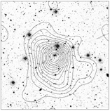
Figure 26: $V$ band light distribution map. The FoV is $\sim 16\arcmin 40\arcsec\times 16\arcmin 40\arcsec$, North is up, East to the Left. The contours correspond to values $2\times 10^{5}$, $2.5\times 10^{5}$, $3\times 10^{5}$, …, $7.5\times 10^{5}$, $8\times 10^{5}$ L_⊙. The light distribution shows one single peak without any distinct substructures. The position difference between the cluster center and the peak of the distribution is about $\sim 29\arcsec$, which might be a result from the masked parts of the image, see Fig. 21)

To calculate the total luminosity in the $V$ band in solar units we assume the solar absolute magnitude to be $\rm M\it_{V}=$4.82mag (Cox, 2000). We also assume the cluster members to follow the standard Schechter luminosity function (Schechter, 1976):

$$\phi(L)dL=\phi^{*}\left(\frac{L}{L^{*}}\right)^{\alpha}e^{-\left(\frac{L}{L^{*}}\right)}d\left(L/L^{*}\right)$$ (12)

In terms of magnitudes the Schechter function reads

$$\phi(M)dM=0.4\ln(10)\cdot\phi^{*}\cdot 10^{-0.4(M-M^{*})(\alpha+1)}\cdot e^{\left[-10^{-0.4(M-M^{*})}\right]}dM$$ (13)

To obtain the parameters $L^{*}$, $\phi^{*}$ and $\alpha$ we applied a $\chi^{2}$ fit to Eq.13 using the MatLab^© Fitting Toolbox at a 95% confidence level. The best fitting parameters including the $\chi^{2}$-value for the goodness of the fit and the fitting range for the luminosity $[\inf,L_{fit}]$ are given in Table 6, where $L_{fit}$ is the completeness luminosity.
The total luminosity $L_{tot}$ (see Table 6) can now be obtained by integrating Eq. 12:

$$L_{tot}=\phi^{*}L^{*}\Gamma(2-\alpha)$$ (14)

The integration of the Schechter function down to a luminosity $L_{\rm lim\it}$ is equal to

$$L_{lim}=\phi^{*}L^{*}\Gamma(2-\alpha,L_{lim}/L^{*}).$$ (15)

As the Schechter function is not applicable to very faint luminosities we calculate the fraction of light we miss due to observational effects

$$F=1-\frac{\Gamma(2-\alpha,L_{fit}/L^{*})}{\Gamma(2-\alpha,L_{lim}/L^{*})}$$ (16)

$L_{fit}$ being the luminosity (corresponding to $M_{fit}$ in Table 6) down to which our catalogues are complete and $L_{lim}$ is the limiting luminosity corresponding to the limiting magnitude given in Table 3.
Fig.26 shows the corresponding light distribution of the Red Sequence galaxies in $V$. Again, only one single, very distinct peak centred on the BCG is visible. In addition the distribution is very smooth and shows no substructures, confirming the relaxed state of Z3146.
In Sect. 5.1.2 we fitted the mass obtained by the weak lensing method to an NFW profile with the following best-fit parameters obtaining $r_{200}=1661^{+280}_{-328}\;h_{70}^{-1}$kpc and $c=3.6^{+2.8}_{-2.4}$ as best fit values. This leads to $M_{200}=7.04^{+6.03}_{-2.32}\times 10^{14}M_{\odot}$. Using these values we find a mass-to-light ratio within $r_{200}$ in the $V$ band of $M/L_{V}\sim 156^{+134}_{-51}M_{\odot}/L_{\odot}$. This value is in agreement with e.g. Hradecky et al. (2000), who give a median value of $M/L_{V}\sim 138M_{\odot}/L_{\odot}$ for eight clusters within a radius of $\sim 1.38\,h_{70}^{-1}$Mpc.

7 Discussion and summary

We presented a combined investigation of optical and X-ray observations of the prominent galaxy cluster Z3146. This cluster seems to be in a relaxed state, which is confirmed by

• the absence of large substructures in the galaxy density plot and the light distribution map (see Fig. 25 and Fig. 26),

• the regular shape of the cluster in the X-ray image and the temperature map (see Fig. 1 and 3, respectively)

• the massive nominal cooling flow of $\sim 1600M_{\odot}$yr^-1

• the good coincidence of the optical, the X-ray, and the weak lensing centre (each of the order of a few arcseconds), and

• the regular shape of the weak lensing mass reconstruction.

Further optical investigations on the cluster also revealed four gravitational arc candidates and a mass-to-light ratio of $M/L_{V}\sim 156^{+134}_{-51}\,\,h_{70}^{-1}M_{\odot}/L_{\odot}$ at $r_{200}=1661^{+280}_{-328}\;h_{70}^{-1}$kpc.

We also determined the mass of this cluster with two independent methods, weak lensing and X-ray measurements. Both data sets, X-ray and lensing, were used to establish best fits to the commonly used NFW model. Fig. 27 shows the comparison of the confidence levels for these data:
Fig. 27(a) - Xray-data: Confidence level from a NFW fit to the mass profile derived from X-ray data according to Eq. 4. The contour levels are 2.31, 6.25, 11.90 corresponding to confidence levels of 68.3% ($1\sigma$), 95.4% ($2\sigma$), 99.73% ($3\sigma$).
Fig. 27(b) - Lensing data: The contours are at $2\Delta{\cal L}=$2.30, 6.17, 9.21 corresponding to confidence levels of 63.8%, 90%, 95.4% and 99% if we assume Gaussian statistics. We varied the galaxy sample of the lensing fit to investigate the dependence of the result on this parameter. On the one hand, lowering the maximum radius to which galaxies enter the calculations to $8\hbox{$.\!\!^{\prime}$}0$ from the galaxy centre (we have full data coverage around the cluster up to this radius; see Fig. 8) leads to $r_{200}=1610\;h_{70}^{-1}$kpc; $c=4.01$. On the other hand, not considering the inner parts of the cluster and using only galaxies with a distance larger than $2\hbox{$.\!\!^{\prime}$}0$ we obtain $r_{200}=1748\;h_{70}^{-1}$kpc; $c=1.0$. We note that $r_{200}$ is reasonably well constrained and that the concentration $c$ mainly depends on the details near the cluster core. This behaviour corresponds to the shape of our contours and is typical for NFW profile fits in weak lensing studies; see e. g. Clowe & Schneider (2002) and Dietrich et al. (2005). The parameter ranges in $c$ and $r_{200}$ imply an uncertainty of the total cluster mass of $10\%-20\%$ (considering radii of $1-2\;h_{70}^{-1}$Mpc; see also Fig. 18).
Fig. 27(c) - Direct Comparison: The ’x’ marks our best fit lensing value of $r_{200}=1661\;h_{70}^{-1}$ kpc ($r_{s}=460.1\;h_{70}^{-1}$ kpc) and $c=3.61$, which lies in the vicinity of the $3\sigma$ X-ray model. The triangle corresponds the best NFW fit to the X-Ray data: $r_{200}=1849\;h_{70}^{-1}$ kpc, $c=3.58$ ($r_{s}=516.6\;h_{70}^{-1}$ kpc, see Sect. 3.5 for more details). This best fit value is located within the $1\sigma$ contour of the lensing model. Hence both models are in excellent agreement.

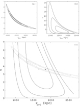
Figure 27: Comparison of confidence levels from NFW fits: Panel (a) shows the fit to the X-ray data, Panel (b) the fit to the shear data. A direct comparison with the corresponding best fit values is presented in Panel (c), where the lensing model is represented by the solid lines (best fit marked by ’x’), and the X-ray model by the dash-dotted lines (best fit values correspond to the triangle). See Sect. 7 for more details.

A direct comparison of the mass profiles and the ratio between $M_{X-ray}/M_{wl}$ is given in Fig. 28, which shows that the best fit models agree within $\sim 20\%$.
Comparing the strong and weak lensing masses it seems that they disagree. At the radius of the outermost arc at $r\sim 27\arcsec$ ($\sim 120$ kpc) we obtain a mass within an Einstein ring of about $M_{\rm sl}=1.39^{+0.36}_{-0.35}\times 10^{14}\,\,h_{70}^{-1}$ M_⊙ for the strong lensing measurement. The NFW profile of the weak lensing fit gives $M_{\rm wl}=2.35^{+2.58}_{-1.56}\times 10^{13}\,\,h_{70}^{-1}$ M_⊙ at the same position, which is, the best case assuming, roughly half of $M_{\rm sl}$ only. However, due to the large uncertainties in the strong lensing mass determination (unknown redshifts, unknown lensing geometry…) we assume this mass only to be a rough upper value. Hence this discrepancy is likely an artifact of the large numbers of uncertainties in the determination of the strong lensing mass.

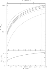
Figure 28: Comparison of the best fit NFW models obtained from X-ray data (black lines) and weak lensing signal (gray lines). Both show good coincidences within 1$\sigma$ errors (see Fig. 27). In the lower panel the ratio of $M_{X-ray}/M_{wl}$ is shown. Note, that the fit of the X-ray data to a NFW profile starts at $\leq 230\;h_{70}^{-1}$kpc. The dash-dotted line represents $r_{200}=1661h_{70}^{-1}$kpc. See Sect. 7 for more details.

Especially in relaxed clusters, the mass estimates obtained from weak lensing and X-ray mass methods usually seem to agree very well (Allen, 1998; Wu et al., 1998). Recent observations of cooling flow clusters derived from Chandra and/or XMM-Newton confirm these results (see e.g. Allen et al., 2002; Cypriano et al., 2005). We find a temperature of $5.9\pm 0.1$ keV in Z3146, in agreement with the assumption of Cypriano et al. (2004) that clusters having an ICM temperature $\lesssim 8.0$ keV are in a relaxed state. In particular relaxed clusters are interesting for cosmological studies as their mass content tends to take a spherically symmetric shape, which is the usual assumption in theoretical approaches. Hence a large sample of such systems is a useful probe to verify whether the mass density of galaxy clusters follows an NFW profile (Navarro et al., 1996, 1997), or whether a different profile like the Burkert (Burkert, 2000), the Moore (Moore et al., 1999) or the non-extensive profile (Leubner, 2005; Kronberger et al., 2006) is a suitable description.