Criticality and Condensation in a Non-conserving Zero Range Process

Abstract

The Zero-Range Process, in which particles hop between sites on a lattice under conserving dynamics, is a prototypical model for studying real-space condensation. Within this model the system is critical only at the transition point. Here we consider a non-conserving Zero-Range Process which is shown to exhibit generic critical phases which exist in a range of creation and annihilation parameters. The model also exhibits phases characterised by mesocondensates each of which contains a subextensive number of particles. A detailed phase diagram, delineating the various phases, is derived.

1 Introduction

There exist many systems exhibiting real-space condensation under nonequilibrium steady state conditions. Examples include jamming in traffic flow, granular clustering, wealth condensation and gelation in networks [1]. Real-space condensation implies that a finite fraction of some conserved quantity, for example density, condenses onto a single lattice site or a small region in space. In general one is interested in the distribution of the conserved quantity and the emergence of the condensate as some parameter, often the density, is varied.

The Zero-Range Process (ZRP) [2] is a generic model which exhibits condensation in its nonequilibrium steady state [3, 4]. Moreover it has the convenient property that its steady state is known and has a simple factorised form. Thus the ZRP provides a simple exactly solvable model within which general features of condensation may be studied and analysed [1]. For example, recent developments include: extensions of the model to several conserved quantities [5, 6, 7], open boundary conditions [8], and sitewise disorder [9, 10, 11]; the study of current fluctuations [12] and traffic modelling [13, 14].

The ZRP is usually defined on a lattice of $L$ sites where each site may be occupied by any integer number of particles. The dynamics is defined by hopping rates $u(n)$ with which a particle hops from a site occupied by $n$ particles. In various versions of the dynamics the particle may hop to different allowed destination sites. For example on a regular lattice particles hop to nearest neighbour sites whereas on a fully-connected geometry a particle can hop to any other site with equal probability. Clearly, the total number of particles, $N$, is conserved under the ZRP dynamics. Condensation occurs when in the large $N$, $L$ limit, with the density $\rho=N/L$ held fixed, a finite fraction of the particles condenses onto a single lattice site. More recently, an example where the condensate has a non-zero spatial extent has been studied [15].

Condensation is revealed in the single-site occupation probability distribution, $p(n)$. A characteristic case is when the hopping rate has the asymptotic, large $n$ form $u(n)\simeq 1+b/n$. For $b>2$, the model exhibits a condensation transition at a critical density $\rho_{c}$. For $\rho<\rho_{c}$, $p(n)$ has the form

$$p(n)\propto n^{-b}{\rm e}^{-\mu n}$$ (1)

where $\mu$ is positive and is a function of the density. Since there is a characteristic occupation this is referred to as the fluid phase.

As the density increases towards the critical value $\rho_{c}$, $\mu$ tends to zero and the resulting distribution becomes a power law at $\rho=\rho_{c}$. For $\rho>\rho_{c}$ an extra piece of $p(n)$, representing a single condensate, emerges centered at $n=L(\rho-\rho_{c})$ [16]. Thus in the condensed phase a critical fluid co-exists with a condensate containing the excess density. A pure power-law distribution only holds at the critical density which is a common feature in many systems exhibiting phase transitions. For $b<2$ there is no condensation transition since any density can be achieved by choosing $\mu$ to be suitably small in (1).

In this work we consider more general dynamical processes which could allow for more complex condensation phenomena. Examples of the phenomena we have in mind are the existence of criticality in an extended region of the phase diagram rather than at an isolated point (typically referred to as self-organised criticality), and condensation into a large number of condensates each containing a subextensive number of particles. In our generalised dynamics we introduce non-conserving processes with creation and annihilation rates. One mechanism to suppress a single extensive condensate is for the annihilation of particles to occur preferentially at highly occupied sites. We find that an appropriate choice of creation and annihilation rates leads to a whole critical region of the phase diagram where the occupation distribution decays algebraically at large occupations. Since the density is not conserved the phase diagram is given in terms of the parameters of the creation and annihilation rates.

Let us briefly summarise the phases which are exhibited (see Fig. 1). As might be expected, for imbalanced creation and annihilation rates we find regimes with vanishing or diverging density. These two regimes are separated by phases where the observed density is equal to what would be the critical density on a conserving system and power-law occupation distributions are exhibited. One of these phases, Critical Phase A, exhibits a pure power-law distribution for $p(n)$ with a cut-off diverging with system size. However another region in parameter space exists where the distribution exhibits, in addition to the power-law decay, a broad and weak peak at high occupations. The height of the peak scales algebraically with system size, rather than exponentially, as does the width. This peak may correspond to many ‘mesocondensates’ each of which contains a subextensive number of particles. The number of these mesocondensates is also subextensive thus they occupy a vanishing fraction of the sites. We shall give a detailed analysis of this weak peak and how it leads to two phases: Critical Phase B where the weak peak does not contribute to the global density which is $\rho_{c}$ and the Weak High Density Phase where the contribution of the weak peak to the global density is dominant.

In a recent publication [17] we gave a brief account of the non-conserving ZRP and its relation to self-organised criticality and the dynamics of rewiring networks. Here we focus on the properties of the non-conserving ZRP and present a detailed analysis of the phase diagram.

The structure of the paper is as follows: in Section 2 we define the non-conserving ZRP that we study; in Section 3 we present a detailed analysis of the phase diagram via a mean-field approximation and we compare the results to numerical simulations on fully-connected and one-dimensional lattices; we conclude with a discussion in Section 4.

2 Definition of non-conserving ZRP

We now define the non-conserving zero-range process which we study in this work. The lattice contains $L$ sites labelled $l=1,\ldots,L$. The number of particles at site $l$ is $n_{l}$. The dynamics are defined by the following three processes: particles hop from a site with $n$ particles with rate

$$u(n)=\left(1+\frac{b}{n}\right)\theta(n)\;,$$ (2)

where the step function $\theta(n)$ is defined as

$$\theta(n)=\left\{\begin{array}[]{c}1\quad\mbox{for}\quad n>0\\ 0\quad\mbox{for}\quad n=0\;,\end{array}\right.$$ (3)

particles are created at a site with rate

$$c=\frac{1}{L^{s}}\;,$$ (4)

and particles evaporate from a site containing $n$ particles with rate

$$a(n)=\left(\frac{n}{L}\right)^{k}\theta(n)\;.$$ (5)

In these rates the indices $k$ and $s$ are positive. The creation rate at a site (4) provides a weak drive which decreases with system size. The particle annihilation rate at a site (5) increases with the number of particles at the site and provides a mechanism by which an extensive condensate may be suppressed.

As noted in the introduction, condensation in the conserving ZRP occurs when $b>2$ and in the following we focus primarily on this range of $b$. For the specific choice of hopping (2) the critical density is known to be [18, 19]

$$\rho_{c}=\frac{1}{b-2}\;.$$ (6)

Note that in the non-conserving case $N$ and consequently the density $\rho$ fluctuate in time.

The precise nature of the lattice and the definition of the sites to which particles are allowed to hop from a given site do not affect the qualitative picture emerging from this study (as long as the lattice is homogeneous with all sites having the same hop rates). To be specific we consider a fully-connected lattice where a particle can hop to any other lattice site. This is a convenient choice, since on the fully-connected lattice the mean-field approach with which we treat the model analytically is expected to become exact in the large system limit. In addition, we shall also present numerical data from one dimensional systems with totally asymmetric nearest neighbour hopping which indicate that the results of the mean-field analysis are relevant to this case as well.

In a Monte-Carlo simulation the dynamics defined in (2–5) are conveniently implemented as follows: At each update

1. Select a site at random.

2. Generate a random number uniformly distributed between zero and the sum of the maximum possible rates of the three processes, i.e., $c+\max(a(n))+\max(u(n))$.

3. If the random number falls in the range $(0,c)$ create a particle at the site.

4. If the random number falls in the range $(c,c+a(n))$, where $n$ is the number of particles on the site, evaporate a particle from the site.

5. If the random number falls in the range $(c+\max(a(n)),c+\max(a(n))+u(n))$ remove a particle from this site and place it at another randomly selected site.

Note, as the evaporation rate $a(n)$ can diverge, a cut-off $\max(a(n))$ must be imposed artificially and chosen large enough that, in practice, the dynamics is not affected.

The steady state of the model is fully described by the probability distribution $P(n_{1},n_{2},\ldots,n_{L})$ over all possible configurations. In contrast to the conserving ZRP [4], the steady-state distribution of the model (2–5) does not factorize generally. However, for the case of a fully-connected lattice we expect factorisation to take effect in the thermodynamic limit $L\to\infty$. In the following analysis we apply a mean field approximation in which the steady state distribution is replaced by a factorized form, i.e. $P(n_{1},n_{2},\ldots,n_{L})\to\prod_{i=1}^{L}p(n_{i})$. For the fully-connected lattice we expect this approximation to become exact in the thermodynamic limit.

Within this approximation, the master equation is given by

$$\frac{\partial p(n)}{\partial t} = \left[u(n+1)+a(n+1)\right]p(n+1)-\left[\lambda+c\right]p(n)$$

$$-\left\{\left[u(n)+a(n)\right]p(n)-\left[\lambda+c\right]p(n-1)\right\}\theta(n)\;.$$

where $p(n)$ is the probability that a site contains $n$ particles. The step function $\theta(n)$ ensures that (2) holds for all $n\geq 0$. The ‘current’ $\lambda$ into a site due to the hopping process is given by

$$\lambda=\sum_{n=1}^{\infty}u(n)p(n)\;.$$ (8)

To understand (2) note that $u(n)+a(n)$ is the total rate at which a site with $n$ particles loses a particle and $\lambda+c$ is the total rate at which a site gains a particle.

In the steady state (2) becomes

$$0 = \left[u(n+1)+a(n+1)\right]p(n+1)-\left[\lambda+c\right]p(n)$$

$$-\left\{\left[u(n)+a(n)\right]p(n)-\left[\lambda+c\right]p(n-1)\right\}\theta(n).$$

which may be iterated to obtain the steady-state $p(n)$

$$p(n)=\frac{(\lambda+c)^{n}}{\prod_{m=1}^{n}[a(m)+u(m)]}p(0)\;.$$ (10)

To fix $p(0)$ and $\lambda$, $p(n)$ must satisfy the following constraints of normalisation and creation–annihilation balance respectively

$$\sum_{n=0}^{\infty}p(n) = 1$$ (11)

$$\sum_{n=1}^{\infty}a(n)p(n) = c\;.$$ (12)

Only two of equations (8), (11) and (12) are independent, as can be seen by noting

$$\left[a(n)+u(n)\right]p(n)=(\lambda+c)p(n-1)\;,$$ (13)

which, when summed, becomes

$$\sum_{n=1}^{\infty}\left[a(n)+u(n)\right]p(n)=(\lambda+c)\sum_{n=0}^{\infty}p(n)=\lambda+c\;.$$ (14)

3 Analysis of phase diagram of non-conserving ZRP

We now determine the asymptotic, large $L$ behaviour of $\lambda$ (and therefore $p(n)$) required to satisfy (8) and (12). We identify a total of five phases in the $s$–$k$ plane: low density phase, strong and weak high density phases and a critical region which itself consists of two distinct critical phases as we shall explain below.

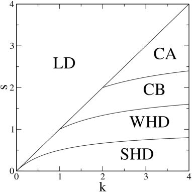
Figure 1: Typical phase diagram for the non-conserving ZRP model, shown in the $k$–$s$ plane for $b=3$. The parameters $k,s,b$ are defined in (2–5). The labelling of the phases corresponds to Low Density Phase (LD), Critical Phase A (CA), Critical Phase B (CB), Weak High Density Phase (WHD) and Strong High Density Phase (SHD).

Identifying the five phases is most conveniently done by inspecting the balance equation (12) which becomes on inserting the expressions (10) for $p(n)$, (4) for $c$ and (5) for $a$

$$L^{k-s} = \sum_{n=1}^{\infty}n^{k}p(n)$$ (15)

$$= p(0)\sum_{n=1}^{\infty}n^{k}\exp\left[n\,{\ln(\lambda+c)}-\sum_{m=1}^{n}\ln(a(m)+u(m))\right]\;.$$

3.1 Low density phase: $s>k$

For $s>k$ the LHS of (15) tends to zero as the system size $L$ tends to infinity. This requires that $p(n)$ is a rapidly decreasing function of $n$. To satisfy the balance equation (15) $\lambda+c$ has to be small. Then to leading order in $L$, $\lambda+c\simeq\lambda\sim L^{k-s}$

$$p(n)\sim L^{-(s-k)n}\;.$$ (16)

Thus the density $\rho\simeq p(1)\sim L^{k-s}$ which tends to zero as the system size tends to $\infty$. The mean total number of particles $N$ increases sublinearly with system size as $L^{k-s+1}$ and so we are in a low density phase when $s>k$.

3.2 Analysis of $s<k$ region

In this case, since $s<k$, the LHS of (15) diverges with $L$, so the sum on the RHS must also diverge and must be dominated by terms at large $n$. This can only happen if $\lambda+c$ approaches one for large $L$. Otherwise, if the limiting value of $\lambda+c$ were less than one the sum would not diverge, whereas if the limiting value were greater than one the sum would diverge even for finite $L$. Therefore we write

$$\lambda+c=1+h(L)\simeq e^{h(L)}\;,$$ (17)

where $h(L)\to 0$ as $L\to\infty$. Since we are interested in the large $n$ behaviour of $p(n)$, keeping leading order terms in $n$, we have $\ln(a(m)+u(m))\simeq b/m+(m/L)^{k}$ and then approximating the sum by an integral gives, for large $n$,

$$\sum_{m=1}^{n}\ln\left[a(m)+u(m)\right]\simeq b\ln(n)+\frac{n^{k+1}}{(k+1)L^{k}}\;.$$

Therefore, from (10), the asymptotic form of $p(n)$ is

$$p(n)\sim\frac{1}{n^{b}}\exp\left[h(L)n-\frac{n^{k+1}}{(k+1)L^{k}}\right]\;.$$ (18)

The rest of the analysis amounts to determining more precisely the large $L$ behaviour of $h(L)$ required to satisfy the balance equation (15) in the various regions of the $s$–$k$ plane.

3.3 Strong High Density Phase: $s<k/(k+1)$

The form of (18) suggests that if $h(L)$ is positive, $p(n)$ may be sharply peaked at some value $n^{*}$ which dominates $p(n)$. By sharply peaked we mean that for $\epsilon$ arbitrarily small, $\int_{n^{*}-\epsilon}^{n^{*}+\epsilon}{\rm d}n\ p(n)\to 1$ as $L\to\infty$. Then the balance equation (15) reduces to $L^{k-s}\simeq(n^{*})^{k}$ which implies

$$n^{*}\simeq L^{1-s/k}\;.$$ (19)

This condition may be used to determine $h(L)$. Maximising the argument of the exponential in (18) yields $n^{*}=Lh^{1/k}(L)$. Therefore comparing with (19) we require

$$h(L)\simeq L^{-s}\;.$$ (20)

However, for the distribution to be sharply peaked at $n^{*}$ we require that the argument of the exponential in (18) diverges for large $L$ at $n^{*}$. Thus, for example, $n^{*}h(L)\simeq L^{1-s-s/k}$ should diverge which implies

$$s<\frac{k}{k+1}\;.$$ (21)

In this phase, note that $\lambda+c=1+O(L^{-s})$ approaches one from above. Also note that the number of particles is super extensive and the mean density is $n^{*}$ which diverges as (19). The sharply peaked distribution $p(n)$ is rather different from that of a conserving ZRP at high density, where a critical fluid and a condensate piece coexist. In contrast, in the present case all sites contain $O(n^{*})$ particles and we refer to this as the Strong High Density Phase.

3.4 Intermediate Regime

We now consider the intermediate regime $k/(k+1)<s<k$ and show that $p(n)$ approaches a power-law distribution. A careful analysis shows that, in fact, this region may be divided into three phases: two of these are critical in the sense that the density is given by $\rho_{c}$, the critical density of the conserving ZRP. The first critical phase (Critical Phase A) has a power-law distribution $p(n)$ with a cut-off at large $n$. The second critical phase (Critical Phase B) has a power-law distribution together with a broad and weak peak at large occupations. In the thermodynamic limit this peak does not contribute to the global density and thus the global density is critical. Finally we have a phase similar to Critical Phase B but where the broad peak dominates the global density which now diverges with $L$. We refer to this as the Weak High Density Phase.

3.4.1 Critical Phase A $(kb/(k+1)\leq s<k)$

In the case where $\lambda+c$ approaches one from below, namely when $h(L)$ in (17) is negative, the distribution (18) becomes a power law with a large $n$ cut-off at $n\sim\mbox{min}[1/|h(L)|,L^{k/(k+1)}]$. This cut-off goes to infinity with $L$ resulting in a power-law distribution in the thermodynamic limit.

We analyse the region in the $s$–$k$ plane where such a behaviour is manifested. Setting $h(L)\simeq-gL^{-x}$, where $g$ is a positive constant, and replacing the sum by an integral, the balance equation (15) takes the form

$$L^{k-s}\sim\int_{1}^{\infty}{\mathrm{d}}n\;n^{k-b}\exp\left[-g\frac{n}{L^{x}}-\frac{n^{k+1}}{(k+1)L^{k}}\right]\;.$$ (22)

In the case $k>b-1$ the integral is dominated by large $n$. The cut-off in the large $n$ contribution will be given by $L^{x}$, as long as $x\leq k/(k+1)$. The asymptotic behaviour of (22) becomes

$$L^{k-s} \sim L^{x(k-b+1)}\;.$$ (23)

Thus, $x$ is given by

$$x=\frac{k-s}{k-b+1}\;.$$ (24)

To be consistent with the requirement $x\leq k/(k+1)$ one finds from (24) that $s$ has to satisfy

$$s \geq \frac{bk}{k+1}\;.$$ (25)

When the equality holds, both terms in the exponential in (22) are relevant. To summarise, in the range $kb/(k+1)\leq s<k$ the asymptotic behaviour of $p(n)$ is a power law with an exponential cut-off, the cut-off point tending to infinity as the system size tends to infinity:

$$p(n)\sim n^{-b}\exp\left[-g\frac{n}{L^{x}}\right]\;,$$ (26)

where $x$ is given by (24), and $g$ is an undetermined positive constant. For this phase to exist we require $k>b-1$.

3.4.2 The region $k/(k+1)\leq s<kb/(k+1)$

This still leaves the behaviour in the region $k/(k+1)<s<kb/(k+1)$ to be determined. We expect that some kind of local maximum in $p(n)$ is needed in order to cope with the increased creation rate in this region compared with Critical Phase A. However, a sharp peak in $p(n)$ is ruled out since that would correspond to the Strong High Density phase. Instead we shall show that a ‘weak peak’ emerges in $p(n)$ whose height scales algebraically with $L$ as opposed to the sharp exponential peak in the high density phase (see Figure 2). We now demonstrate the existence of such a peak in the distribution in the region $k/(k+1)<s<kb/(k+1)$, and show how it satisfies the balance equation (15).

\psfrag{nstar}{$n^{*}$}\psfrag{nmin}{$n_{\mathrm{min}}$}\psfrag{pofnstar}{$p(n^{*})$}\psfrag{deltanstar}{$\Delta n^{*}$}\includegraphics[width=199.16928pt]{weakpeak.eps}

Figure 2: Schematic illustration of a weak peak in $p(n)$. Note that both the height $p(n^{*})$ and width $\Delta n^{*}$ scale algebraically with system size $L$ but the weight. $w=\Delta n^{*}p(n^{*})$ of the peak vanishes. The dip in the distribution to the left of the weak peak is denoted $n_{\rm min}$.

Let us write the distribution (18) as

$$p(n)\sim e^{\psi(n)}$$ (27)

where

$$\psi(n)=h(L)n-\frac{1}{k+1}\frac{n^{k+1}}{L^{k}}-b\ln n\;.$$ (28)

We now seek a function $h(L)$ which produces a maximum at $n^{*}$ and for which $\psi(n^{*})\sim\ln L$. This would result in $p(n^{*})$ scaling as a power of $L$. In order for the second term in (28) to scale as $\ln L$ we require $n^{*}\sim(L^{k}\ln L)^{1/(k+1)}$. Then for the first term to scale similarly we require

$$h(L)=\left(\frac{d\ln L}{L}\right)^{k/(k+1)}\;,$$ (29)

where $d$ is some constant to be determined. Having deduced the required functional form of $h(L)$ we now turn to determining the constant $d$ and the precise location and properties of the weak peak.

Taking the first two derivatives of $\psi(n)$ we have

$$\psi^{\prime}(n) = \left(\frac{d\ln L}{L}\right)^{k/(k+1)}-\frac{n^{k}}{L^{k}}-\frac{b}{n}$$ (30)

$$\psi^{\prime\prime}(n) = -k\frac{n^{k-1}}{L^{k}}+\frac{b}{n^{2}}\;.$$ (31)

Setting $\psi^{\prime}(n^{*})=0$, gives to leading order in $L$

$$n^{*} \simeq d^{1/(k+1)}L^{k/(k+1)}\left(\ln L\right)^{1/(k+1)}\;,$$ (32)

$$\psi(n^{*}) \simeq \frac{(d-b)k}{k+1}\ln L-\frac{b}{k+1}\ln\ln L\;,$$ (33)

$$\psi^{\prime\prime}(n^{*}) \simeq -kL^{-2k/(k+1)}\left(\ln L\right)^{(k-1)/(k+1)}d^{(k-1)/(k+1)}\;.$$ (34)

These expressions imply that the height of the peak at $n^{*}$ is

$$p(n^{*})\sim L^{k(d-b)/(k+1)}\left(\ln L\right)^{-b/(k+1)}\;,$$ (35)

and the width of the peak is given by

$$\Delta n^{*}=\left|\psi^{\prime\prime}(n^{*})\right|^{-1/2}\sim L^{k/(k+1)}\left(\ln L\right)^{-(k-1)/(2(k+1))}\;.$$ (36)

Thus the weight $w$ of the weak peak in $p(n)$, which we define as

$$w=p(n^{*})\Delta n^{*}$$ (37)

is given by

$$w\sim L^{(d-b+1)k/(k+1)}(\ln L)^{-(k-1+2b)/2(k+1)}\;.$$ (38)

The balance equation (15) is satisfied by the contribution of the weak peak and becomes asymptotically,

$$L^{k-s}\sim(n^{*})^{k}w\;.$$ (39)

Inserting the expressions (38) and (32) implies, ignoring logarithmic factors,

$$d=b-\frac{s\,(k+1)}{k}\;.$$ (40)

Thus, from (18), $p(n)$ behaves asymptotically as

$$p(n)\sim n^{-b}\exp\left[n\left\{\left(b-\frac{s(k+1)}{k}\right)\frac{\ln L}{L}\right\}^{k/(k+1)}-\frac{n^{k+1}}{(k+1)L^{k}}\right]\;.$$ (41)

When $s<kb/(k+1)$ one has $d>0$ as required. Also we require that the weight (38) of the peak should not diverge as $L\to\infty$ otherwise the system would be in the Strong High Density Phase. This implies from (38) and (40) that $s\geq k/(k+1)$.

To summarise, for $k/(k+1)\leq s<kb/(k+1)$ we have a probability distribution which initially decreases from a finite $p(0)$ as a power law as in Critical Phase A, but with a weak peak at high $n$. The weak peak allows the creation-annihilation balance condition to be satisfied (see Fig 2). At this point let us recap the properties of the weak peak, ignoring logarithmic correction factors:

$$n^{*} \sim \Delta n^{*}\sim L^{k/(k+1)}$$ (42)

$$p(n^{*}) \sim L^{-s}$$ (43)

$$w \sim L^{k/(k+1)-s}\;.$$ (44)

Within the region $k/(k+1)\leq s<kb/(k+1)$ there are in fact two phases distinguished by the behaviour of the global density. To see this we note that the number of particles per site, $n_{wp}$, associated with the weak peak is

$$n_{wp}\simeq n^{*}w\sim L^{2k/(k+1)-s}$$ (45)

This gives the contribution of the weak peak to the density. Clearly this contribution diverges or goes to zero according to whether or not $s<2k/(k+1)$, thus implying two distinct regimes.

Critical Phase B: $2k/(k+1)<s<kb/(k+1)$
In this region $n_{wp}$ approaches zero in the large $L$ limit and the global density of the system is controlled by the power law part of $p(n)$. Thus the global density is $\rho=\rho_{c}$ where $\rho_{c}$ is the critical density of the corresponding conserving ZRP (6).

Weak High Density Phase: $k/(k+1)\leq s<2k/(k+1)$
In this region $n_{wp}$ diverges so the density is dominated by the weak peak and the total number of particles increases as $N\sim L^{2k/(k+1)-s+1}$.

In these two phases most of the sites of the system form a fluid with typically low occupation numbers. In addition a subextensive number of sites, $Lw\sim L^{1-s+k/(k+1)}$ are highly occupied with $n\simeq n^{*}$ particles where $n^{*}\sim L^{k/(k+1)}$ diverges sublinearly with $L$. We term these highly occupied sites mesocondensates. The expected number of such mesocondensates is given by $wL\sim L^{1-s+k/(k+1)}$ which can vary from $O(L)$ to $O(L^{1-k(b-1)/(k+1)})$. If

$$b>2+\frac{1}{k}\;,$$ (46)

the average number of mesocondensates can be very much less than one. Thus, in this case we typically do not expect to observe any mesocondensates. In terms of $s$, this happens when

$$\frac{kb}{k+1}>s>\frac{2k+1}{k+1}\;.$$ (47)

Another distinction between Critical Phase A and the phases characterised by a weak peak is the behaviour of arbitrary moments of $n$

$$\mu_{r}=\int{\rm d}n\,n^{r}p(n)\;.$$ (48)

In Critical Phase A $\mu_{r}$ diverges when $r>b-1$. On the other hand, the contribution to $\mu_{r}$ from a weak peak is $(n^{*})^{r}w\sim L^{(r+1)/(k+1)-s}$ which diverges when $r>s(k+1)/k-1$. Therefore in Critical Phase B and the Weak High Density Phase which moments diverge depends on the precise values of $s,k$. This is in contrast to Critical Phase A where throughout the phase the same moments ($\mu_{r}$ for $r>b-1$) diverge.

3.5 Summary of phase diagram

We have identified the following phases which are illustrated in a typical phase diagram in Figure 1

• $k<s$ — Low Density Phase (LD)

  Here $p(n)$ decays as $L^{-(s-k)n}$ and the global density vanishes as $L^{-(s-k)}$.

• $kb/(k+1)\leq s<k$ — Critical Phase A (CA)

  Here $p(n)$ decays algebraically as $1/n^{b}$ with a cut-off at $L^{y}$ where $y=(k-s)/(k-b+1)$. The global density throughout this phase is the critical density $\rho_{c}$.

• $2k/(k+1)\leq s<bk/(k+1)$ — Critical Phase B (CB)

  Here $p(n)$ decays algebraically as $1/n^{b}$ and is cut-off by a weak peak, with properties (42–44), at $n^{*}\sim(\ln L)^{1/(k+1)}L^{k/(k+1)}$. The global density is the critical density $\rho_{c}$.

• $k/(k+1)\leq s<2k/(k+1))$ — Weak High Density Phase (WHD)

  Here $p(n)$ decays algebraically as $1/n^{b}$ and is cut-off by a weak peak at $n^{*}\sim(\ln L)^{1/(k+1)}L^{k/(k+1)}$. The global density diverges as $\rho\sim L^{2k/(k+1)-s}$

• $s<k/(k+1)$ — Strong High Density Phase (SHD)

  Here $p(n)$ is sharply peaked around $n^{*}\sim L^{1-s/k}$ and the global density diverges as $n^{*}$.

Numerical evidence for these phases is presented in Figure 3 and Figure 4. In Figure 3 typical distributions $p(n)$ for the phases with non-zero density are presented and compare favourably with the theoretical predictions. The theoretical predictions were generated by taking the predicted asymptotic forms of $\lambda$ and inserting into (10). In the case of Critical Phase A, the constant $g$ was taken to be 1 although, $g$ could be used as a parameter to improve the fit to the simulation data. In Figure 4, $p(n)$ is plotted in Critical Phase A for different $L$ illustrating the $L$ dependence of the cut-off.

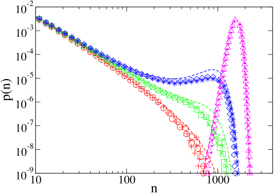
Figure 3: Steady-state distributions of the number of particles on a site from simulations of the non-conserving ZRP model on a fully connected lattice (open shapes) and a 1d lattice (character symbols), compared with theoretical curves (dashed lines). Simulations were run on a system with L=5000 lattice sites and $b=2.6$, $k=3$. Data are shown for: Critical Phase A, $s=2$ (${\color[rgb]{1,0,0}\circ}$, ${\color[rgb]{1,0,0}+}$ and - -); Critical Phase B, $s=1.7$ (${\color[rgb]{0,1,0}\Box}$, ${\color[rgb]{0,1,0}\times}$ and - -); Weak High Density Phase, $s=1.2$ (${\color[rgb]{0,0,1}\Diamond}$, ${\color[rgb]{0,0,1}*}$ and - -); Strong High Density Phase, $s=0.4$ (${\color[rgb]{1,0,1}\triangle}$, ${\color[rgb]{1,0,1}\bullet}$ and - -).

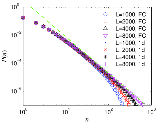
Figure 4: Steady state probability distributions from simulations in Critical Phase A, illustrating $L$ dependence of the cut-off. Here $b=2.6$, $k=3$ and $s=2$, with $L=1000$, 2000, 4000, 8000. The legend indicates for each data set the system size and the geometry used: fully-connected lattice (FC) or one-dimensional lattice (1d). The dashed line corresponds to $P(n)\sim n^{-b}$.

3.6 Nearest Neighbour Hopping

As noted above we expect the mean-field approximation to be applicable to the fully-connected lattice in the limit $L\to\infty$. We also carried out numerical simulations of the model on a one-dimensional lattice with totally asymmetric hops to nearest neighbour sites and periodic boundary conditions. The results are given in Figure 3 and Figure 4 and compare well with the mean-field predictions.

3.7 The case $b<2$

As noted in the introduction, in the conserving model with $b<2$ condensation does not occur. For the non-conserving model the mean-field analysis follows closely that presented above. One finds that Critical Phase B no longer exists and Critical Phase A becomes a Weak High Density Phase. Thus for $b<2$ one no longer has critical phases and the phase diagram reduces to Low Density, Weak High Density and Strong High Density Phases with phase boundaries given by $s=k$ and $s=k/(k+1)$.

4 Discussion

In this work we have studied a ZRP with non-conserving dynamics by means of a mean-field theory. For the choice of rates (2–5) we find a rich phase diagram with five distinct phases. For low creation rate we find a low density phase with exponentially decaying single-site occupation distribution. On the other hand at high particle creation rate we find a strong high density phase where the single-site occupation is sharply peaked at a large occupation which diverges with system size.

The most interesting phases are in the intermediate region. Here we find two distinct critical phases and a weak high density phase. In the Critical Phase A the occupation distribution decays algebraically with occupation number with a finite-size cut-off which diverges with system size. On the other hand in Critical Phase B there exists a weak but broad peak at large occupation in addition to the algebraic decay. The height and width of this peak scale algebraically with system size and the area under the peak vanishes. This peak corresponds to a large, but subextensive, number of mesocondensates each containing a large but subextensive number of particles. The contribution of this peak to the global density vanishes in the thermodynamic limit leaving the global density as $\rho_{c}$. In addition to these two phase we find a Weak High Density Phase whose structure is very similar to Critical Phase B except that the contribution of the weak peak to the global density is dominant and the global density diverges.

Since the ZRP is a prototypical model for condensation phenomena, we might expect the phases established here to be displayed in other driven systems. It would be of interest to explore this possibility by studying other microscopic models. For example $p(n)$ given in (10) is related to the single-site weight that would be obtained in a conserving ZRP with hop rate given by $\tilde{u}(n)=u(n)+a(n)$. This would imply a conserving ZRP with non monotonic hop rates. Studies of this conserving model have revealed that the phenomenon of multiple condensates exists there as well [20].

References

References

- [1] M.R. Evans and T. Hanney, Nonequilibrium statistical mechanics of the zero-range process and related models, J. Phys. A 38, R195 (2005)
- [2] F. Spitzer, Interaction of Markov processes, Adv. Math. 5, 246 (1970)
- [3] O.J. O’Loan, M.R. Evans and M.E. Cates, Jamming transition in a homogeneous, one-dimensional system: The bus route model, Phys. Rev. E 58, 1404 (1998)
- [4] M.R. Evans, Phase transitions in one-dimensional nonequilibrium systems, Braz. J. Phys. 30, 42 (2000)
- [5] M.R. Evans and T. Hanney, Phase transition in two-species zero-range process, J. Phys. A: Math. Gen 36, L441 (2003)
- [6] S Großkinsky and H Spohn, Stationary measures and hydrodynamics of zero range processes with several species of particles, Bulletin of the Brazilian Mathematical Society 34, 489 2003
- [7] C. Godrèche, E. Levine and D. Mukamel, J. Phys. A: Math. Gen. 38, L523 (2005)
- [8] E. Levine, D. Mukamel, G.M. Schutz Zero-range process with open boundaries J. Stat. Phys. 120, 759 - 778 (2005)
- [9] M R Evans Bose-Einstein condensation in disordered exclusion models and relation to traffic flow Europhys. Lett., 36 13-18 (1996)
- [10] J Krug, Phase separation in disordered exclusion models, Braz. J. Phys., 30 97 (2000)
- [11] K Jain and M Barma Dynamics of a Disordered, Driven Zero-Range Process in One Dimension Phys. Rev. Lett. 91, 135701 (2003)
- [12] R. J. Harris, A. Rákos, G. M. Schütz Current fluctuations in the zero-range process with open boundaries J. Stat. Mech. P08003 (2005)
- [13] E. Levine, G. Ziv, L. Gray and D. Mukamel, Physica A 340, 636, (2004); J. Stat. Phys 117, 819, (2004)
- [14] J. Kaupužs, R. Mahnke and R.J. Harris, Zero-range model of traffic flow, Phys. Rev. E 72, 056125 (2005)
- [15] M. R. Evans, T. Hanney, Satya N. Majumdar Interaction driven real-space condensation Phys. Rev. Lett. 97, 010602 (2006)
- [16] S.N. Majumdar, M. R. Evans and R. K. P. Zia Phys. Rev. Lett. 94, 180601 (2005); M. R. Evans, S.N. Majumdar and R. K. P. Zia J. Stat. Phys. 123, 357 (2006)
- [17] A.G. Angel, M.R. Evans, E. Levine and D. Mukamel, Critical phase in non-conserving zero-range processes and equilibrium networks, Phys. Rev. E 72, 046132 (2005)
- [18] S. Großkinsky, G.M. Schütz and H. Spohn, Condensation in the zero-range process: stationary and dynamical properties, J. Stat. Phys. 113, 389 (2003)
- [19] C. Godrèche, Dynamics of condensation in zero-range processes, J. Phys. A 36, 6313 (2003)
- [20] Y Schwarzkopf Masters Thesis, Weizmann Insitute (2006)