Identities by Generalized $L-$Summing Method

Abstract.

In this paper, we introduce 3-dimensional $L-$summing method, which is a rearrangement of the summation $\sum A_{abc}$ with $1\leq a,b,c\leq n$. Applying this method on some special arrays, we obtain some identities on the Riemann zeta function and digamma function. Also, we give a Maple program for this method to obtain identities with input various arrays and out put identities concerning some elementary functions and hypergeometric functions. Finally, we introduce a further generalization of $L-$summing method in higher dimension spaces.

1. Introduction and Motivation

Consider the following $n\times n$ multiplication table

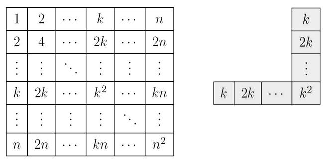
Figure 1. Multiplication table and $L-$summing element, $L_{k}$

If we set $\Sigma(n)$ for the sum of all numbers in it, then by summing line by line we have $\Sigma(n)=\left(\frac{n(n+1)}{2}\right)^{2}$. On the other hand, we can find $\Sigma(n)$ by using another method; letting $L_{k}$ be the sum of numbers in the rotated $L$ in above table (right part of Figure 1), we have

$$L_{k}=k+2k+\cdots+k^{2}+\cdots+2k+k=2k(1+2+\cdots+k)-k^{2}=k^{3}.$$

We call $L_{k}$, $L-$summing element. Thus we get $\Sigma(n)=\sum_{k=1}^{n}L_{k}=\sum_{k=1}^{n}k^{3}$, and therefore $\sum_{k=1}^{n}k^{3}=\left(\frac{n(n+1)}{2}\right)^{2}$. This is 2-dimensional L-summing method (applied on the array $A_{ab}=ab$), which briefly is

(1.1) $$\sum(L-{\rm Summing~{}Elements})=\Sigma.$$

More precisely, the $L-$summing method of elements of $n\times n$ array $A_{ab}$ with $1\leq a,b\leq n$, is the following rearrangement

$$\sum_{k=1}^{n}\left\{\sum_{a=1}^{k}A_{ak}+\sum_{b=1}^{k}A_{kb}-A_{kk}\right\}=\sum_{1\leq a,b\leq n}A_{ab}.$$

This method allows to obtain easily some classical algebraic identities and also, with help of MAPLE, some new compact formulas for sums related with the Riemann zeta function, the gamma function and the digamma function [2, 3].
In this paper we introduce a 3-dimensional version of $L-$summing method for $n\times n\times n$ arrays and applying it on some special arrays we obtain some identities concerning the Riemann zeta function and digamma function. Then, we give a Maple program for this method and using it we generate and then proof some new identities, concerning some elementary functions and hypergeometric functions. Finally, we introduce a further generalization of $L-$summing method in higher dimension spaces and for latices related by a manifold.

2. Formulation of the $L-$summing method in $\mathbb{R}^{3}$

Consider a three dimensional array $A_{abc}$ with $1\leq a,b,c\leq n$ and $n$ is a positive integer. We should prepare an explicit version of the general formulation (1.1) for this array. The summation of all entries is $\Sigma(n)=\sum_{1\leq a,b,c\leq n}A_{abc}$. The $L-$summing elements in this array have the form pictured bellow

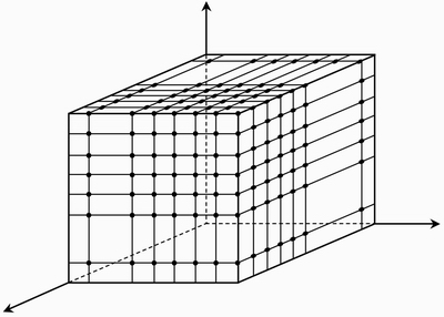
Figure 2. $L-$summing elements in $\mathbb{R}^{3}$

So, we have $L_{k}=\Sigma_{2}-\Sigma_{1}+\Sigma_{0}$, with

$$\Sigma_{2}=\sum_{b,c=1}^{k}A_{kbc}+\sum_{a,c=1}^{k}A_{akc}+\sum_{a,b=1}^{k}A_{abk},\hskip 28.45274pt\Sigma_{1}=\sum_{a=1}^{k}A_{akk}+\sum_{b=1}^{k}A_{kbk}+\sum_{c=1}^{k}A_{kkc},\hskip 28.45274pt\Sigma_{0}=A_{kkk}.$$

Therefore, $L-$summing method in $\mathbb{R}^{3}$ take the following formulation

(2.1) $$\sum_{k=1}^{n}\{\Sigma_{2}-\Sigma_{1}+\Sigma_{0}\}=\Sigma(n).$$

Note that $\Sigma_{2}$ is the sum of entries in three faces, $\Sigma_{1}$ is the sum of entries in three intersected edges and $\Sigma_{0}$ is the end point of all faces and edges.
If the array $A_{abc}$ is symmetric, that is for each permutation $\sigma\in S_{3}$ it satisfies $A_{abc}=A_{\sigma(a)\sigma(b)\sigma(c)}$, then $L-$summing elements in $\mathbb{R}^{3}$ takes the following easier form

(2.2) $$L_{k}=3\sum_{1\leq b,c\leq k}A_{kbc}-3\sum_{a=1}^{k}A_{akk}+A_{kkk}.$$

In the next section we will apply 3-dimensional $L-$summing method on two special symmetric arrays, related by the Riemann zeta function and digamma function.

3. Arrays related by the Riemann zeta function and digamma function

3.1. The Riemann zeta function

Suppose $s\in\mathbb{C}$ and let $A_{abc}=(abc)^{-s}$. It is clear that

$$\Sigma(n)=\sum_{1\leq a,b,c\leq n}(abc)^{-s}=\left(\sum_{k=1}^{n}\frac{1}{k^{s}}\right)^{3}=\zeta_{n}^{3}(s),$$

where $\zeta_{n}(s)=\sum_{k=1}^{n}k^{-s}$. Since this array is symmetric, considering (2.2), we have

$$L_{k}=3\frac{\zeta_{k}^{2}(s)}{k^{s}}-3\frac{\zeta_{k}(s)}{k^{2s}}+\frac{1}{k^{3s}},$$

and an easy simplifying, we can reform $\sum L_{k}=\Sigma(n)$ as follows

(3.1) $$\sum_{k=1}^{n}\frac{\zeta_{k}^{2}(s)}{k^{s}}-\frac{\zeta_{k}(s)}{k^{2s}}=\frac{\zeta_{n}^{3}(s)-\zeta_{n}(3s)}{3}.$$

Note that if $\Re(s)>1$, then $\lim_{n\rightarrow\infty}\zeta_{n}(s)=\zeta(s)$, where $\zeta(s)=\sum_{k=1}^{\infty}n^{-s}$ is the well-known Riemann zeta function defined for complex values of $s$ with $\Re(s)>1$ and admits a meromorphic continuation to whole complex plan [5]. So, for $\Re(s)>1$ we have

$$\sum_{k=1}^{\infty}\frac{\zeta_{k}^{2}(s)}{k^{s}}-\frac{\zeta_{k}(s)}{k^{2s}}=\frac{\zeta^{3}(s)-\zeta(3s)}{3},$$

which also is true for other values of $s$ by meromorphic continuation, except $s=1$ and $s=\frac{1}{3}$.

3.2. Digamma function

Setting $s=1$ in (3.1) (or equivalently taking $A_{abc}=\frac{1}{abc}$) and considering $\zeta_{n}(1)=H_{n}=\sum_{k=1}^{n}\frac{1}{k}$, we obtain

$$\sum_{k=1}^{n}\frac{H_{k}^{2}}{k}-\frac{H_{k}}{k^{2}}=\frac{H_{n}^{3}-\zeta_{n}(3)}{3}.$$

One can state this identity in sense of digamma function $\Psi(x)=\frac{d}{dx}\ln\Gamma(x)$, with $\Gamma(x)=\int_{0}^{\infty}e^{-t}t^{x-1}dt$ is the well-known gamma function. Considering logarithmic derivative of the formula $\Gamma(n+1)=n\Gamma(n)$, we obtain

(3.2) $$\Psi(n+1)=\frac{1}{n}+\Psi(n),$$

and applying this relation, we yield that $\Psi(n+1)-\Psi(1)=H_{n}$. Thus, we have

(3.3) $$\Psi(n+1)+\gamma=H_{n},$$

in which $\gamma=0.57721\cdots$ is the Euler constant [1]. Therefore, we obtain

(3.4) $$\sum_{k=1}^{n}\left\{\frac{(\Psi(k+1)+\gamma)^{2}}{k}-\frac{\Psi(k+1)+\gamma}{k^{2}}\right\}=\frac{(\Psi(n+1)+\gamma)^{3}-\zeta_{n}(3)}{3}.$$

Letting

$$\mathfrak{S}(m,n)=\sum_{k=1}^{n}\frac{\Psi(k)^{m}}{k},$$

the following identity [3] is a result of 2-dimensional $L-$summing method

(3.5) $$\mathfrak{S}(1,n)=\frac{(\Psi(n+1)+\gamma)^{2}+\Psi(1,n+1)}{2}-\frac{\pi^{2}}{12}-\Psi(n+1)\gamma-\gamma^{2},$$

where $\Psi(m,x)=\frac{d^{m}}{dx^{m}}\Psi(x)$ is called $m^{th}$ polygamma function [1] and we have $\sum_{k=1}^{n}\frac{1}{k^{2}}=-\Psi(1,n+1)+\frac{\pi^{2}}{6}$, which is special case of the following identity

(3.6) $$\zeta_{n}(s)=\frac{(-1)^{s-1}}{(s-1)!}\Psi(s-1,n+1)+\zeta(s)\hskip 28.45274pt(s\in\mathbb{Z},s\geq 2),$$

and using it in (3.1) one can get a generalization of (3.4), however this relation itself is the key of getting an analogue of (3.5) in ${\mathbb{R}}^{3}$, stated bellow.

Theorem 3.1.

For every integer $n\geq 1$, we have

$$\sum_{k=1}^{n}\frac{\Psi(k)^{2}}{k}+\frac{\Psi(k)}{k^{2}}=\frac{(\Psi(n+1)+\gamma)^{3}}{3}-\frac{\zeta_{n}(3)}{3}+(\gamma-2)\frac{\pi^{2}}{6}-(\gamma-2)\Psi(1,n+1)-\gamma^{2}\Psi(n+1)-\gamma^{3}-2\mathfrak{S}(1,n).$$

Proof.

We begin from the left hand side of the identity (3.4); simplifying it by the relations (3.2), (3.3) and the relation (3.6) with $s=2$, gives the result. ∎

Corollary 3.2.

For every integer $n\geq 1$, we have

$$\mathfrak{S}(2,n)=\frac{(\Psi(n+1)+\gamma)^{3}}{3}-\frac{\zeta_{n}(3)}{3}+(\gamma-2)\frac{\pi^{2}}{6}-(\gamma-2)\Psi(1,n+1)-\gamma^{2}\Psi(n+1)-\gamma^{3}-2\mathfrak{S}(1,n)-\sum_{k=1}^{n}\frac{\Psi(k)}{k^{2}}.$$

In above corollary, the main term in the right hand side is $\frac{\Psi(n+1)^{3}}{3}$. Also, we note that the summation $\sum_{k=1}^{n}\frac{\Psi(k)}{k^{2}}$ is converges. Thus, we can write the following asymptotic relation

$$\mathfrak{S}(2,n)=\frac{\Psi(n+1)^{3}}{3}+O(\ln^{2}n)\hskip 28.45274pt(n\rightarrow\infty).$$

Similarly, considering (3.5) we have

$$\mathfrak{S}(1,n)=\frac{\Psi(n+1)^{2}}{2}+O(\ln n)\hskip 28.45274pt(n\rightarrow\infty).$$

Note and Problem. It is interesting to find an explicit (probably recurrence) relation for the function $\mathfrak{S}(m,n)$. Considering two above asymptotic relations, we guess that

$$\mathfrak{S}(m,n)=\frac{\Psi(n+1)^{m+1}}{m+1}+O(\ln^{m}n)\hskip 28.45274pt(n\rightarrow\infty).$$

One can attack to this problem considering generalization of $L-$summing method in higher dimension spaces, pointed in the last section of this paper.

4. Generating some new identities by Maple and 3-dimension $L-$summing method

Appendix of this paper includes Maple program of 3-dimension $L-$summing method. By $\textit{{LSMI}}<A_{abc}>$, we call the identity outputted by $L-$Summing method’s Maple program with input $A_{abc}$. The algorithm of this program is result of the formulation of 3-dimension $L-$summing method in above sections. In this program we input a 3-dimensional array $A_{abc}$, then out put is an identity generated by Maple. In this section we will state some of these identities, with handling a detailed proof.

4.1. Some elementary functions

Proposition 4.1.

We have

$$\texttt{LSMI}<\ln(a)>:\sum_{k=1}^{n}\left\{{k}^{2}\ln k+2\,k\ln\Gamma(k+1)-2\,k\ln k-\ln\Gamma(k+1)+\ln k\right\}={n}^{2}\ln\Gamma(n+1).$$

Proof.

Considering the relations (2.1) and $\Gamma(n+1)=n!$, we have $\Sigma(n)=n^{2}\sum_{a=1}^{n}\ln a=n^{2}\ln\Gamma(n+1)$. Also, $\Sigma_{2}=k^{2}\ln k+2k\ln\Gamma(k+1)$, $\Sigma_{1}=\ln\Gamma(k+1)+2k\ln k$ and $\Sigma_{0}=\ln k$. Putting these relations in (2.1) yields $\textit{{LSMI}}<\ln(a)>$ as desired. ∎

Corollary 4.2.

We have

$$\sum_{k=1}^{n}\left\{(k^{2}-k)\ln k+2k\ln\Gamma(k+1)\right\}=(n^{2}+n)\ln\Gamma(n+1).$$

Proof.

Breaking up the statement under the summation obtained from $\textit{{LSMI}}<\ln(a)>$ in Proposition 4.1, into the sum of $(k^{2}-k)\ln k+2k\ln\Gamma(k+1)$ and $\ln\Gamma\left(k+1\right)+k\ln k-\ln k$, and considering the Proposition 6 of [3], which states

$$\sum_{k=1}^{n}\left\{\ln\Gamma\left(k+1\right)+k\ln k-\ln k\right\}=n\ln\Gamma(n+1),$$

completes the proof. ∎

Remark 4.3.

Examining Maple code of expressed summation on above corollary, one can see that Maple has no comment on the computing this summation; however, it is obtained by Maple itself and $L-$summing method. This example shows that program-writers of Maple can add $L-$summing method in the summation package of this software, in order to making it able to compute some summations which already couldn’t compute them.

Proposition 4.4.

A little simplifying $\texttt{LSMI}<\tan(a)>$, we have

$$\sum_{k=1}^{n}\left\{(k-1)^{2}\tan k+(2k-1)\mathfrak{T}(k)\right\}=n^{2}\mathfrak{T}(n),$$

where $\mathfrak{T}(n)=\sum_{k=1}^{n}\tan k$.

Proof.

Considering the relation (2.1), we have $\Sigma(n)=n^{2}\sum_{a=1}^{n}\tan a=n^{2}\mathfrak{T}(n)$. Also, $\Sigma_{2}=k^{2}\tan k+2k\mathfrak{T}(k)$, $\Sigma_{1}=\mathfrak{T}(k)+2k\tan k$ and $\Sigma_{0}=\tan k$, and consequently $L_{k}=(k-1)^{2}\tan k+(2k-1)\mathfrak{T}(k)$. This completes the proof. ∎

4.2. Hypergeometric functions

In the next proposition, we introduce an identity concerning hypergeometric functions, denoted in Maple by $\texttt{hypergeom([}a_{1}~{}~{}a_{2}~{}\cdots~{}a_{p}\texttt{],[}b_{1}~{}~{}b_{2}~{}\cdots~{}b_{q}\texttt{],}x\texttt{)}$. Standard notation and definition [6] is as follows

$$~{}_{p}F_{q}\left[\begin{array}[]{cccc}a_{1}&a_{2}&\cdots&a_{p}\\ b_{1}&b_{2}&\cdots&b_{q}\end{array};x\right]=\sum_{k\geq 0}t_{k}x^{k},$$

where

$$\frac{t_{k+1}}{t_{k}}=\frac{(k+a_{1})(k+a_{2})\cdots(k+a_{p})}{(k+b_{1})(k+b_{2})\cdots(k+b_{q})(k+1)}x.$$

Proposition 4.5.

A little simplifying $\texttt{LSMI}<a!>$ and stating in standard notations, we have

$$\sum_{k=1}^{n}\left\{(k-1)^{2}k!+(2k-1)(k+1!)\mathfrak{H}(1,k+2)\right\}=n^{2}(n+1)!\mathfrak{H}(1,n+2),$$

where

$$\mathfrak{H}(\alpha,\beta)=~{}_{2}F_{0}\left[\begin{array}[]{cc}\alpha&\beta\\ -\end{array};1\right].$$

Proof.

Considering definition of hypergeometric functions we have $\mathfrak{H}(1,n+1)=(n+1)\mathfrak{H}(1,n+2)$, which implies $\sum_{a=1}^{n}a!=\mathfrak{H}(1,2)-(n+1)!\mathfrak{H}(1,n+2)=\mathfrak{P}(n)$, say. This gives $\Sigma(n)=n^{2}\mathfrak{P}(n)$ and in similar way it yields that $L_{k}=(k-1)^{2}k!+(2k-1)\left((k+1!)\mathfrak{H}(1,k+2)-\mathfrak{H}(1,2)\right)$. Thus, we obtain

$$\sum_{k=1}^{n}\left\{(k-1)^{2}k!+(2k-1)\left((k+1!)\mathfrak{H}(1,k+2)-\mathfrak{H}(1,2)\right)\right\}=n^{2}(n+1)!\mathfrak{H}(1,n+2)-n^{2}\mathfrak{H}(1,2),$$

and a easy simplifying this, implies the result. ∎

Remark 4.6.

Three last propositions are examples of the array $A_{abc}=f(a)$, for some given function $f$. In this case, $L-$summing method takes the following form

$$\sum_{k=1}^{n}\left\{(2k-1)\mathfrak{F}(k)+(k-1)^{2}f(k)\right\}=n^{2}\mathfrak{F}(n),$$

where $\mathfrak{F}(n)=\sum_{a=1}^{n}f(a)$.

5. Further generalizations of the $L-$summing method and some comments

5.1. The $L-$Summing method in ${\mathbb{R}}^{t}$

Consider a $t-$dimensional array $A_{x_{1}x_{2}\cdots x_{t}}$ and let $\Sigma(n)=\sum A_{x_{1}x_{2}\cdots x_{t}}$ with $1\leq x_{1},x_{2},\cdots,x_{t}\leq n$. The $L-$Summing method in ${\mathbb{R}}^{t}$ is the rearrangement $\Sigma(n)=\sum L_{k}$, where $L_{k}=\sum_{m=1}^{t}\left\{(-1)^{m-1}\Sigma_{t-m}\right\}$ and

$$\Sigma_{t-m}=\sum_{1\leq i_{1}<i_{2}<\cdots<i_{m}\leq t}\left\{{\sum}^{\prime}A_{\textbf{x}_{i_{1}i_{2}\cdots i_{m}}}\right\},$$

where in the inner summation ${\sum}^{\prime}$ is over $x_{j}\in\{x_{i_{1}},\cdots,x_{i_{m}}\}^{C}=\{x_{1},x_{2},\cdots,x_{t}\}-\{x_{i_{1}},\cdots,x_{i_{m}}\}$ with $1\leq x_{j}\leq k$, and the index $\textbf{x}_{i_{1}i_{2}\cdots i_{m}}$ denotes $x_{1}x_{2}\cdots x_{t}$ with $x_{i_{1}}=x_{i_{2}}=\cdots=x_{i_{m}}=k$. One can apply this generalized version to get more general form of relations obtained in previous sections. For example, considering the array $A_{x_{1}x_{2}\cdots x_{t}}=(x_{1}x_{2}\cdots x_{t})^{-s}$ with $s\in\mathbb{C}$, yields

$$\sum_{k=1}^{n}\left\{\sum_{m=1}^{t-1}(-1)^{m-1}{t\choose m}k^{-ms}\zeta_{k}(s)^{t-m}\right\}=\zeta_{n}(s)^{t}+(-1)^{t}\zeta_{n}(ts).$$

5.2. $L-$summing method on manifolds

As in rising of this paper, the base of the $L-$summing method is ordinary multiplications table. Above generalization of the $L-$Summing method in ${\mathbb{R}}^{t}$ is based on generalized multiplication tables [4]. But, $\mathbb{R}^{t}$ is a very special $t$-dimensional manifold, and if we replace it with $\Gamma$, an $l-$dimensional manifold with $l\leq t$, then we can define generalized multiplication table on $\Gamma$ by considering lattice points on it (which of course isn’t easy problem). Let

$$L_{\Gamma}(n)=\big{\{}(a_{1},a_{2},\cdots,a_{t})\in\Gamma\cap\mathbb{N}^{t}:1\leq a_{1},a_{2},\cdots,a_{t}\leq n\big{\}},$$

and $f:\mathbb{R}^{k}\longrightarrow\mathbb{C}$ is a function. If $\mathcal{O}_{\Gamma}$ is a collection of $k-1$ dimension orthogonal manifolds, in which $L_{\Gamma}(n)=\cup_{\Lambda\in\mathcal{O}_{\Gamma}}L_{\Lambda}(n)$ and $L_{\Lambda_{i}}(n)\cap L_{\Lambda_{j}}(n)=\phi$ for distinct $\Lambda_{i},\Lambda_{j}\in\mathcal{O}_{\Gamma}$, then we can formulate $L-$summing method as follows,

$$\sum_{X\in L_{\Gamma}(n)}f(X)=\sum_{\Lambda\in\mathcal{O}_{\Gamma}}\left\{\sum_{X\in L_{\Lambda}(n)}f(X)\right\}.$$

Here $L-$summing elements are $\sum_{X\in L_{\Lambda}(n)}f(X)$. This may be useful when one apply it on some special manifolds.

5.3. Stronger form of $L-$summing method

One can state the method of $L-$summing $\sum L_{k}=\Sigma(n)$ in the following stronger form

$$L_{n}=\Sigma(n)-\Sigma(n-1).$$

Specially, this will be useful for those arrays with $\Sigma(n)$ computable explicitly and $L_{k}$ maybe note. For example, applying this note on the array $A_{x_{1}x_{2}\cdots x_{t}}=(x_{1}x_{2}\cdots x_{t})^{-s}$ in ${\mathbb{R}}^{t}$ with $s\in\mathbb{C}$, implies

$$\sum_{m=1}^{t-1}(-1)^{m-1}{t\choose m}n^{-ms}\zeta_{n}(s)^{t-m}=\zeta_{n}(s)^{t}+(-1)^{t}\zeta_{n}(ts)-\zeta_{n-1}(s)^{t}-(-1)^{t}\zeta_{n-1}(ts).$$

 

Appendix. Maple Program of 3-dimension $L-$Summing Method for the array $A_{abc}=\frac{1}{abc}$

restart:
A[abc]:=1/(a*b*c);
S21:=sum(sum(eval(A[abc],a=k),b=1..k),c=1..k):
S22:=sum(sum(eval(A[abc],b=k),a=1..k),c=1..k):
S23:=sum(sum(eval(A[abc],c=k),a=1..k),b=1..k):
S2:=S21+S22+S23:
S11:=sum(eval(eval(A[abc],a=k),b=k),c=1..k):
S12:=sum(eval(eval(A[abc],a=k),c=k),b=1..k):
S13:=sum(eval(eval(A[abc],b=k),c=k),a=1..k):
S1:=S11+S12+S13:
S0:=eval(eval(eval(A[abc],a=k),b=k),c=k):
L[k]:=simplify(S2-S1+S0):
ST(A):=(simplify(sum(sum(sum(A[abc],a=1..n),b=1..n),c=1..n))):
Sum(L[k],k=1..n)=ST(A);

$$A_{abc}:=\frac{1}{abc}$$

$$\sum_{k=1}^{n}{\frac{3\,\left(\Psi\left(k+1\right)\right)^{2}{k}^{2}+6\,\Psi\left(k+1\right){k}^{2}\gamma+3\,{\gamma}^{2}{k}^{2}-3\,\Psi\left(k+1\right)k-3\,\gamma\,k+1}{{k}^{3}}}=\left(\Psi\left(n+1\right)+\gamma\right)^{3}$$

References

-
[1]
M. Abramowitz and I.A. Stegun, HANDBOOK OF MATHEMATICAL
FUNCTIONS: with Formulas, Graphs, and Mthematical Tables, Dover
Publications, 1972.
Available at: http://www.convertit.com/Go/ConvertIt/Reference/AMS55.ASP - [2] Jacek Gilewicz (Reviewer), Review of the paper [3] (in this reference list), Zentralblatt MATH Database, European Mathematical Society, FIZ Karlsruhe & Springer-Verlag, 2007.
- [3] M. Hassani, Identities by L-summing Method, Int. J. Math. Comp. Sci., Vol. 1 (2006) no. 2, 165-172.
- [4] M. Hassani, Lattice Points and Multiplication Tables, Int. J. Contemp. Math. Sci., Vol. 1 (2006) no. 1, 1-2.
- [5] Aleksandar Ivic, The Riemann Zeta Function, John Wiley & sons, 1985.
-
[6]
M. Petkovšek, H.S. Wilf and D. Zeilberger, , A. K. Peters,
1996.
Available at: http://www.cis.upenn.edu/ wilf/AeqB.html