Geometry of Borromean Halo Nuclei
Abstract
We discuss the geometry of the highly quantal nuclear three-body systems composed of a core plus two loosely bound particles. These Borromean nuclei have no single bound two-body subsystem. Correlation plays a prominent role. From consideration of the value extracted from electromagnetic dissociation, in conjunction with HBT-type analysis of the two valence-halo particles correlation, we show that an estimate of the over-all geometry can be deduced. In particular we find that the opening angle between the two neutrons in 6He and 11Li are, respectively, and . These angles are reduced by about 12 to and if the laser spectroscopy values of the rms charge radii are used to obtain the rms distance between the cores and the center of mass of the two neutrons. The opening angle in the case of 11Li is more than 20 larger than recently reported by Nakamura Nak06 . The analysis is extended to 14Be and the two-proton Borromean nucleus 17Ne where complete data is still not available. Using available experimental data and recent theoretical calculations we find, and , respectively.
pacs:
21.45.+v, 25.60.-t, 21.10.KyBorromean nuclei are fragile three-body systems with all two-body sub-systems being unbound. Typical examples are 6He, 11Li and 14Be which are two-neutron Borromean halo isotopes and 17Ne which is a two-proton Borromean halo isotope of neon. The reason that the two-body subsystems are unbound while the three-body system is bound is entirely due to the effective (in-medium) two-nucleon correlations. How strong are these effective two-body correlations? Do they correspond to di-nucleon systems, where spatial correlations are maximum, or to some kind of a Cooper correlation, where the two nucleons sit at opposite sides of the core?
From the experimental point of view, the answer to this question could be obtained from a concomitant measurement of the values and source size in a Hanbury-Brown-Twiss (HBT) type correlation study HB56 . We will argue here that this scheme should supply a mean of estimating the average value of the opening angle between the halo nucleons in Borromean nuclei.
In a recent publication, Nakamura et al. Nak06 studied the low lying dipole excitation in 11Li. Nakamura’s work has had a great impact in this field because new results, showing deviations from previous experimental analysis, have been reported Nak06 . They also deduced the opening angle between the two neutrons in the halo. By relating their measured to the rms value of the distance between the core, 9Li and the center of mass of the two valence neutrons, viz
| (1) | ||||
| (2) | ||||
and using obtained from the no-correlation value of () given in Ref. EB92 using a dipole sum rule value, namely e2fm2, Nakamura et al. Nak06 obtained for the value
Notice that the simple relation, Eq. (1), used by Nakamura has a very simple interpretation in terms of . When one gets . This is because the two valence nucleons lie on opposite sides of the nucleus and the dipole operator vanishes identically due to their same charge-to-mass ratio. On the other hand, it , i.e. when the valence nucleon wavefunctions agglomerate close to each other (dineutron), one gets a maximum value of . Thus, assuming the validity of the three-body model for the Borromean nucleus, without the complications of effective charges, core-polarization, etc., the experimental values of are valuable telltales of the nuclear geometry.
A similar procedure can be employed for the other Borromean nuclei when data are available. However, the method of Nakamura relies on the use of the no-correlation value of , and thus is heavily model-dependent. Namely, from Ref. EB92 , one has with (no nn correlation),
| (3) |
The above equation supplies a value for if the Dipole Sum Rule (DSR) value of , , is used.
| (4) |
For 11Li e2fm2 EB92 . Nakamura et al. Nak06 then used the above value of in eq. 3, with their experimental value of , , after setting
| (5) |
where the average of the product is approximated by the product of averages
| (6) |
With eq. 5, and with the further assumption and , we get the Nakamura prescription for determining , i.e.
| (7) |
which gives the value for quoted above.
The above procedure is strongly model-dependent as it relies on only one set of experimental observables, , obtained from Coulomb excitation measurements. Clearly, to reduce the model dependence one needs more sets of experimental observables. It is thus very important to seek other observables in order to determine, in a less model dependent way, , for Borromean nuclei. In this article we will focus on this endeavor. We avoid the use of eq. 2 altogether.
In the work of Marques et al. Mar00 ; Mar01 , the two neutron correlation function is measured. This function is defined as
| (8) |
where is the one-neutron momentum distribution and is the two-neutron momentum distribution. The indices 1 and 2 attached to the momenta refer to first and second emitted neutrons. The authors of refs. Mar00 ; Mar01 compared the measured with eq. 8 with an analytical expression for extracted from ref. Led82 to account for the case of direct two-neutron independent emission from a Gaussian source. From such analysis approximate, model-dependent, values of were determined for 6He, 11Li and 14Be. We should stress that the above HBT analysis was based on the use of a simple model of the emission of the two neutrons from a supposed random source. It is not yet clear how large are the coherent effects, and how much these effects would affect the final results of the analysis. Furthermore, the HBT probes the average n-n configuration of the continuum states and not the ground state, as the nucleus is excited above the threshold before the emission occurs. Bearing all of the above in mind, one would only hope to use the HBT results to get, at most, an estimate of the average value of . For a recent review containing, among other things, an account of the difficulties encountered in the correlation measurement and the extraction of , see ref. Nigel .
In what follows we will use the HBT study results for the distance between the two neutrons, given by Marques et al. Mar00 ; Mar01 and show that the opening angle between the two neutrons in 11Li is 25% larger than the above. We also calculate the opening angle for 6He, where full measurement is available (both the , laser spectroscopy and the HBT analysis) and also supply the value of this angle for 14Be as well as for 17Ne using available data and model calculations. We find using the laser spectroscopy data on the rms values of the charge radiiSAN06 , WAN04 and ESB07 , = , and 64 degrees for 11Li, 6He and 14Be, respectively.
For the two-proton Borromean nucleus, 17Ne we use the general cluster formula for the dipole strength function BBH91
| (9) |
with , and obtain
We supply the details of our calculation in what follows.
The experimental analysis of Ref. Mar00 and Mar01 , can be summarized by giving the average distances between the valence nucleons obtained through two-particle correlations that supplies the size of the source. The obtained values are = 6.6 fm, 5.9 fm and 5.6 fm, for 11Li, 6He and 14Be, respectively. From the calculation of Gri06 , one extracts = 4.45 fm.
| (fm) | (fm) | (fm) | B(E1) (fm2) | ||
|---|---|---|---|---|---|
| 6He | 5.9 | 3.36 (39) | 2.67 | 1.20 (20) | 83 |
| Mar00 | Au99 | (2.48) | Au99 | ||
| 3.71(07) | 2.78 | 78 | |||
| WAN04 | |||||
| 11Li | 6.6 | 5.01 (32) | 3.17 | 1.42 (18) | 66 |
| Mar00 | Nak06 | (3.12) | Nak06 | ||
| 5.97(22) | 3.4 | 58 | |||
| SAN06 | |||||
| 14Be | 5.60 | 4.50 | 3.10 | 1.69∗ | 64 |
| Mar01 | ZT95 | (3.16) | ZT95 | ||
| 17Ne | 4.45 | 1.55 | 2.70 | 1.56∗ | 110∘ |
| Gri06 | Gri06 | (2.75) | Gri06 |
From the measured for 6He Au99 and for 11Li Nak06 and the calculated ones for 14Be ZT95 and for 17Ne Gri06 , and using Eq. 1, the rms value of , which is identified as , the average distance between the cm of the core and the cm of the two nucleons, is determined to be 3.36(39), 5.01(32), 4.50 and 1.55 fm, respectively. More accurate values of this latter quantity can be obtained ESB07 from measurements of the rms charge radii SAN06 , WAN04 . They supply for for 6He WAN04 and 11Li SAN06 employing the analysis of ESB07 the values 3.71(07) and 5.97(22), respectively. Moreover, the rms value of is the quantity measured in the HBT studies. From these two experimentally determined and theoretically calculated quantities, the opening angle is approximately obtained without resort to any further model dependence (besides the model dependence of the measured ) except for the assumption .
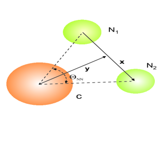
Given and , can one determine the opening angle ? From fig. 1 it is easy to write
| (10) |
The rms value of the cosine above clearly does not correspond to the cosine of the average value of the angle, . This latter can be estimated from
| (11) |
The calculation of the rms value of the cosine in eq. 10 can be performed using the Gaussian model for the source. For our purposes in this paper we use instead eq. 11 to get the already reported estimates of .
How does our current analysis of the geometry of the ground state of Borromean nuclei bear on the values of the rms matter radii tabulated in Oz01 ? To answer this, we use the formula for the rms radius of a two-cluster nucleus, where the two halo nucleons are treated as an extended entity of radius /2,
| (12) |
We have used the radii of the cores, , , and fm, all taken from Oz01 . With the values of cited above and from the measured ’s we find = 2.67(36) fm, 3.17(27) fm, 3.10 fm and 2.70 fm, for the Borromean nuclei 6He, 11Li, 14Be and 17Ne, respectively. These values are to be compared to the tabulated ones given in Oz01 , namely, fm, fm, fm and fm, respectively. Our results are summarized in table I. We did not indicate the error bars in the radius of 17Ne since no data are available.
If we use the values of extracted from the rms charge radii of 6He and 11Li (see above) we get for the rms matter radii the values 2.78 and 3.4 fm, respectively. These values are larger than those of Oz01 but closer to the ones obtained by improved Glauber calculation of the reaction cross sections. For example To97 obtained the value 3.5(6) fm for 11Li.
We should reiterate here a point already mentioned in the paper:the HBT probes the average n-n configuration of the continuum states and not the ground state, as the nucleus is excited above the threshold before the emission occurs. It is therefore expected that the values of corresponding to the ground state would be smaller than the ones quoted in the text and the table. This will result in smaller opening angles, perhaps within the range the errors already indicated in the table.
It is worth mentioning here that the opening angles we have obtained for 6He and 11Li are consistent with the recent three-body pairing calculation of Hagino and Sagawa HS05 .
Notwithstanding the large size of the error bars in the measured and the small difference (2∘) between for 11Li and 14Be, this implies that there is a gradual increase in the intensity of spatial correlations between the two halo neutrons. The case of 17Ne is quite different; owing to the Coulomb repulsion between the two protons the above trend ceases to operate. This may be traced to the scattering lengths of the two nucleon pairs. For the nn case one has the so far accepted value of = -18.6 (4) fm Mil90 ; Bau05 . Though charge symmetry says that the nuclear (hadronic) value of should be equal to that of , the presence of electromagnetic repulsion and other effects render almost one third of . Precisely Mil90 ; Bau66 , one has = -7.8063 (26) fm. It would be quite interesting to check the above by performing both measurement and HBT correlation analysis for the 17Ne two-proton Borromean nucleus. Such an endeavor is currently in the planning stage at the GSI Au07 . Due to the long-range Coulomb interaction, the HBT analysis has to be carried out with care for charged particles BHV07 .
It is tempting to compare our finding for the opening angle between the two halo protons in 17Ne with the opening angle between the two hydrogen atoms in the water molecule H2O. This latter angle is quite well known and its value is , almost equal the nuclear counterpart, . In H2O, pm and pm (pico meter). Though the physics is different, we believe that several universal properties may be common in these quantum three-body systems Jen04 , one of which is the Efimov effect; the limit of infinite -wave scattering length of at least one of the two-body subsystems. This allows for the existence of infinite number of three-body bound states close to the two-body threshold even in the absence of two-body bound states. Such states have been experimentally observed as giant recombination resonances that deplete the Bose-Einstein condensate in cold Cs gases Kr06 . In our present case we are finding a similarity in the three-body geometry of H2O and 17Ne (p2O) which lures us to call 17Ne the nuclear “water” molecule.
In conclusion we have supplied an estimate of the geometry of the Borromean nuclei, 6He, 11Li, 14Be and 17Ne using available values of and the average distance between the valence nucleons supplied by two-particle correlation HBT-type analysis. We have found that the opening angle between the valence nucleons seems to evolve in a decreasing fashion as the mass of the system increases in the case of two-neutron Borromean nuclei. This conclusion is however not definite as it is hampered by the error bars in the measured values of Mar00 ; Mar01 . In the case of the two-proton Borromean halo nucleus 17Ne, the opening angle was found to be , large enough to suggest that the pp sub-system in this nucleus is close to be a Cooper pair Ha06 , in contrast to the nn sub-systems in the two-neutron Borromean nuclei referenced above, where the corresponding nn opening angles were found to be much smaller. After completing a first version of this paper, we became aware of a similar work completed quite recently by Hagino and Sagawa Ha07 . They deduced opening angles for 6He, 11Li close to ours.
Acknowledgements.
We would like to thank Thomas Aumann for very valuable comments. This work was partially supported by the CNPq and FAPESP and by the U.S. Department of Energy under contract No. DE-AC05-00OR22725, and DE-FC02-07ER41457 (UNEDF, SciDAC-2). M. S. H. is the Martin Gutzwiller Fellow 2007/2008.References
- (1) T. Nakamura et al., Phys. Rev. Lett. 96, 252502 (2006).
- (2) R. Hanbury-Brown and R. Q. Twiss, Nature ( London) 178, 1046 ( 1956); S. E. Koonin, Phys. Lett. 70 B, 43 (1977); S. Pratt, Phys. Rev. Lett. 53, 1219 (1984); W. Bauer, C. K. Gelbke and S. Pratt, Ann. Rev. Nucl. Part. Sci. 42, 77 (1992).
- (3) H. Esbensen and G. F. Bertsch, Nucl. Phys. A542, 310 (1992).
- (4) F. M. Marqués et al., Phys. Lett. B 476, 219 (2000).
- (5) F. M. Marqués et al., Phys. Rev. C 64, 061301 (2001).
- (6) R. Lednicky and L. Lyuboshits, Sov. J. Nucl. Phys. 35, 770 (1982).
- (7) N. Orr, Mod. Phys. Lett. A21, 2503 (2006).
- (8) C. A. Bertulani, G. Baur and M. S. Hussein, Nucl. Phys. A 526, 751 (1991); C. A. Bertulani, M. S. Hussein and G. Muenzenberg, Physics of Radioactive Beams (Nova Science Publishing Co. New York, 2001), Chapter 7.
- (9) L. V. Grigorenko, K. Langanke, N. B. Shulgina and M. V. Zhukov, Phys. Lett. B 641, 254 (2006).
- (10) A. Ozawa, T. Suzuki and I. Tanihata, Nucl. Phys. A 693, 32 (2001).
- (11) G. A. Miller, B. M. K. Nefkens and I. Slaus, Phys. Rep. 194, 1 (1990).
- (12) C. Baumer et al., Phys. Rev. C 71, 044003 (2005).
- (13) E.Baumgartner, H. E. Conzett, E. Shield and R. J. Slobodrian, Phys. Rev. 16, 105 (1966).
- (14) T. Aumann, private communication.
- (15) K. Hagino, H. Sagawa, J. Carbonell and P. Schuck, Phys. Rev. Lett. 99, 022506 (2007)..
- (16) T. Aumann et al., Phys. Rev. C 59, 1252 (1999).
- (17) M. V. Zhukov and I. J. Thompson, Phys. Rev. C 52, 3505 (1995).
- (18) K. Hagino and H. Sagawa, Phys. Rev. C 72, 044321 (2005)
- (19) C.A. Bertulani, M.S. Hussein and G. Verde, “Blurred femtoscopy with two-particle emission”, to be published.
- (20) R. Sanchez et al., Phys. Rev. Lett. 96, 033002 (2006).
- (21) L.-B. Wang et al., Phys. Rev. Lett. 93, 142501 (2004).
- (22) H. Esbensen, K. Hagino, P. Mueller and H. Sagawa, Phys. Rev. C 76, 024302 (2007)
- (23) A. S. Jensen, K. Riisager, D. V. Federov and E. Garrido, Rev. Mod. Phys. 76, 215 (2004).
- (24) T. Kraemer et al., Nature 440, 315 (2006).
- (25) K. Hagino and H. Sagawa, arXiv:0708.1543.
- (26) J. A. Tostevin et al., Nucl. Phys. A 616, 418c (1997).