Resonance in an open quantum dot system with a Coulomb interaction:
a Bethe-ansatz approach

Abstract

An open quantum system consisting of a quantum dot with a Coulomb interaction and two leads without interactions is studied. The many-body scattering states are constructed with the Bethe-ansatz approach. The expectation value of the electric current is exactly calculated for the scattering states to observe resonance peaks due to many-body scattering.

The purpose of this letter is to observe resonance in an open quantum system with a Coulomb interaction. The system that we study is the two-lead interacting resonant-level model (IRLM), which consists of two leads of non-interacting electrons that interact with an electron on a quantum dot in between the two leads. We obtain $N$-electron scattering states for arbitrary $N$, generalizing the Bethe-ansatz approach to open systems. By using the scattering states, we exactly calculate the quantum-mechanical expectation value of the electric current through the quantum dot, thereby observing resonance peaks. Some of the resonance peaks appear only when the interaction exists; they reflect the effect of many-body scattering.

The resonance of many-body scattering that we observe in the quantum-mechanical expectation value has not been found in previous works with the Bethe ansatz. The Bethe-ansatz approach has provided a nonperturbative method of studying equilibrium states of interacting quantum systems including the Kondo problem [1, 5, 3, 2, 4]. The approach is now used to discuss transport properties of mesoscopic systems. Konik et al. [7, 6] studied transport properties of the Anderson model in the thermodynamic limit of a closed system with periodic boundary conditions. Our scattering states, in contrast, appear only in open systems; they are constructed without imposing periodic boundary conditions. By extending the Bethe-ansatz approach, Mehta and Andrei [8] studied the two-lead IRLM as an open system to obtain $N$-electron scattering states giving nonequilibrium steady states in the limit $N\to\infty$. In their study, however, the quantum-mechanical expectation value of the current does not depend on the interaction; the effect of the interaction appears only in the statistical-mechanical expectation value as modification of the Fermi distribution in the leads. Thus our results are different from the previous ones.

There has recently been a great deal of interest in mesoscopic systems with interacting electrons. Experiments suggest that interactions are essential in understanding their transport properties [12, 13, 11, 10, 9]. The perturbation theory tells us that the effect of interactions is observed as resonance peaks of the electrical conductance [14, 15]. For non-interacting open quantum systems, the relation between quantum mechanical scattering states and nonequilibrium steady states is well investigated [16, 17]. However, the relation in interacting open quantum systems has not been clarified, excepting Schiller and Hershfield’s result [18] at a special point of the interaction parameter where an interacting system is mapped to a non-interacting one. The present study gives a steady step toward an exact analysis of interacting open quantum systems out of equilibrium.

The Hamiltonian of the two-lead IRLM is given by

$$H\!=\! \sum_{i=1,2}\Big{(}\!\int_{-\frac{L}{2}}^{\frac{L}{2}}dz\hskip 1.0ptc^{\dagger}_{i}(z)\frac{1}{\mathrm{i}}\frac{d}{dz}c_{i}(z)+\frac{t}{\sqrt{2}}\big{(}c^{\dagger}_{i}(0)d\!+\!d^{\dagger}c_{i}(0)\big{)}\Big{)}$$

$$+\epsilon_{d}d^{\dagger}d+U\sum_{i=1,2}c^{\dagger}_{i}(0)c_{i}(0)d^{\dagger}d,$$ (1)

where $t(>0)$ is the transfer integral between each lead and the quantum dot, $\epsilon_{d}$ is the gate energy of the dot and $U(>0)$ expresses the Coulomb repulsion. The dispersion relation in the leads is linearized in the vicinity of the Fermi energy to be $E=k$, under the assumption that $t$, $\epsilon_{d}$ and $U$ are small compared with the Fermi energy [1, 5, 3]. We stress that we treat the system as an open system in the limit $L\to\infty$. The one-lead IRLM with periodic boundary conditions was studied with the Bethe ansatz [3]. Our purpose is to investigate, for scattering states, the electric current through the quantum dot,

$$I\!:=\!\dot{N_{2}}\!-\!\dot{N_{1}}\!=\!\frac{t}{\sqrt{2}\mathrm{i}}\sum_{i=1,2}(-)^{i}\big{(}c_{i}^{\dagger}(0)d-d^{\dagger}c_{i}(0)\big{)}.$$ (2)

We derive the Schrödinger equations for the system. After the transformation $c_{1/2}(z)=\big{(}c_{e}(z)\pm c_{o}(z)\big{)}/\sqrt{2}$, the Hamiltonian (Resonance in an open quantum dot system with a Coulomb interaction: a Bethe-ansatz approach) is decomposed into the even and odd parts [8]. Due to the relations $[H,N_{e}+N_{d}]=[H,N_{o}]=0$ for the number operators $N_{e/o}=\int dzc_{e/o}^{\dagger}(z)c_{e/o}(z)$ and $N_{d}=d^{\dagger}d$, the set $(N_{e}+N_{d},N_{o})$ gives a good quantum number. The $N$-electron state in the subspace with $N_{o}=n,(0\leqslant n\leqslant N)$ is generally expressed in the form

$$|\psi\rangle =\Big{(}\!\int\!\!dz\,g^{(n)}(z)c^{\dagger}_{e}(z_{1})\cdots c^{\dagger}_{e}(z_{N-n})c^{\dagger}_{o}(z_{N-n+1})\cdots c^{\dagger}_{o}(z_{N})$$

$$\quad+\!\int\!\!dz\,e^{(n)}(z)c^{\dagger}_{e}(z_{1})\cdots c^{\dagger}_{e}(z_{N-n-1})d^{\dagger}c^{\dagger}_{o}(z_{N-n})\cdots c^{\dagger}_{o}(z_{N-1})\Big{)}|0\rangle,$$ (3)

where $g^{(n)}(z)=g^{(n)}(z_{1},\ldots,z_{N})$ for $0\leqslant n\leqslant N$ and $e^{(n)}(z)=e^{(n)}(z_{1},\ldots,z_{N-1})$ for $0\leqslant n\leqslant N-1$ are functions to be determined. We also set $e^{(N)}(z)=0$ for convenience. The eigenvalue problem $H|\psi\rangle=E|\psi\rangle$ is cast into a set of the Schrödinger equations

$$(N-n)\Big{(}\sum_{i=1}^{N}\frac{1}{\mathrm{i}}\frac{\partial}{\partial z_{i}}\!-\!E\Big{)}g^{(n)}(z)+t\sum_{i=1}^{N-n}(-)^{N-n-i}\delta(z_{i})e^{(n)}(\ldots,z_{i-1},z_{i+1},\ldots)=0,$$

$$\Big{(}\sum_{i=1}^{N}\frac{1}{\mathrm{i}}\frac{\partial}{\partial z_{i}}\!-\!E\Big{)}g^{(N)}(z)=0,$$

$$\Big{(}\sum_{i=1}^{N-1}\Big{(}\frac{1}{\mathrm{i}}\frac{\partial}{\partial z_{i}}\!+\!U\delta(z_{i})\Big{)}\!+\!\epsilon_{d}\!-\!E\Big{)}e^{(n)}(z)\!+\!t(N\!-\!n)g^{(n)}(\ldots,z_{N-n-1},0,z_{N-n},\ldots)=0,$$ (4)

where $0\leqslant n\leqslant N\!-\!1$. In what follows, we use the variables $x_{i}$ and $y_{i}$ to express the coordinates of the leads $e$ and $o$, respectively: $g^{(n)}(z)=g^{(n)}(x_{1},\ldots,x_{N-n},y_{1},\ldots,y_{n})$ and $e^{(n)}(z)=e^{(n)}(x_{1},\ldots,x_{N-n-1},y_{1},\ldots,y_{n})$. The set of eigenfunctions in the one-electron sector with $E=k$ is given by

$$g^{(0)}(x_{1})=g_{k}(x_{1}):=\frac{2\mathrm{e}^{\mathrm{i}kx_{1}}}{1+\mathrm{e}^{\mathrm{i}\delta_{k}}}\big{(}\theta(-x_{1})+\mathrm{e}^{\mathrm{i}\delta_{k}}\theta(x_{1})\big{)},$$

$$e^{(0)}=e_{k}:=\frac{t}{k-\epsilon_{d}},$$

$$g^{(1)}(y_{1})=h_{k}(y_{1}):=\frac{2\mathrm{e}^{\mathrm{i}ky_{1}}}{1+\mathrm{e}^{\mathrm{i}\delta_{k}}}$$

with the phase shift $\delta_{k}:=-2\arctan\big{(}t^{2}/2(k-\epsilon_{d}))$ of one-body scattering at $x_{1}=0$ in the lead $e$ and the step function $\theta(z)$. Note that the eigenfunction $g_{k}(x_{1})$ is discontinuous at $x_{1}=0$.

We construct an $N$-electron eigenstate with the Bethe ansatz. It is different from the one obtained by Mehta and Andrei [8]. To demonstrate the difference, we first consider the case $N=2$. The set of two-electron eigenfunctions with the energy eigenvalue $E=k_{1}+k_{2}$ is assumed to be

$$2g^{(0)}_{k_{1}k_{2}}(x_{1},x_{2})=Z_{k_{1}k_{2}}(x_{1}-x_{2})g_{k_{1}}(x_{1})g_{k_{2}}(x_{2})-Z_{k_{1}k_{2}}(x_{2}-x_{1})g_{k_{2}}(x_{1})g_{k_{1}}(x_{2}),$$

$$e^{(0)}_{k_{1}k_{2}}(x_{1})=Z_{k_{1}k_{2}}(x_{1})g_{k_{1}}(x_{1})e_{k_{2}}\!-\!Z_{k_{1}k_{2}}(-x_{1})g_{k_{2}}(x_{1})e_{k_{1}},$$

$$g^{(1)}_{k_{1}k_{2}}(x_{1},y_{1})=X(x_{1}-y_{1})g_{k_{1}}(x_{1})h_{k_{2}}(y_{1}),$$

$$e^{(1)}_{k_{1}k_{2}}(y_{1})=X(-y_{1})e_{k_{1}}h_{k_{2}}(y_{1}),$$

$$2g^{(2)}_{k_{1}k_{2}}(y_{1},y_{2})=h_{k_{1}}(y_{1})h_{k_{2}}(y_{2})\!-\!h_{k_{2}}(y_{1})h_{k_{1}}(y_{2}),$$ (5)

where the amplitudes $Z_{k_{1}k_{2}}(z)$ and $X(z)$ are defined by

$$Z_{k_{1}k_{2}}(z):=\mathrm{e}^{-\frac{\mathrm{i}}{2}\varphi_{k_{1}k_{2}}}\theta(-z)+\mathrm{e}^{\frac{\mathrm{i}}{2}\varphi_{k_{1}k_{2}}}\theta(z),$$

$$X(z):=\mathrm{e}^{\frac{\mathrm{i}}{2}\eta}\theta(-z)+\mathrm{e}^{-\frac{\mathrm{i}}{2}\eta}\theta(z)$$

with the phase shifts $\varphi_{k_{1}k_{2}}:=2\arctan\big{(}\!-\!\frac{U}{2}\frac{k_{1}-k_{2}}{k_{1}+k_{2}-2\epsilon_{d}}\big{)}$ and $\eta:=2\arctan(-U/2)$ of two-body scattering. The eigenfunctions $g^{(0)}_{k_{1}k_{2}}(x_{1},x_{2})$ and $e^{(0)}_{k_{1}k_{2}}(x_{1})$ are the same Bethe eigenfunctions as those assumed in the one-lead IRLM [3], although we do not impose periodic boundary conditions. The eigenfunctions $g^{(1)}_{k_{1}k_{2}}(x_{1},y_{1})$ and $e^{(1)}_{k_{1}k_{2}}(y_{1})$ are obtained with separation of variables; if we set $g^{(1)}_{k_{1}k_{2}}(x_{1},y_{1})=X(x_{1}-y_{1})\tilde{g}^{(1)}_{k_{1}k_{2}}(x_{1},y_{1})$ and $e^{(1)}_{k_{1}k_{2}}(y_{1})=X(-y_{1})\tilde{e}^{(1)}_{k_{1}k_{2}}(y_{1})$, Eqs. (Resonance in an open quantum dot system with a Coulomb interaction: a Bethe-ansatz approach) are decoupled into even and odd parts, and the eigenfunctions $\tilde{g}^{(1)}_{k_{1}k_{2}}(x_{1},y_{1})$ and $\tilde{e}^{(1)}_{k_{1}k_{2}}(y_{1})$ are given by the product of eigenfunctions of the even and the odd parts. The eigenfunctions $g^{(2)}_{k_{1}k_{2}}(y_{1},y_{2})$ should be a free fermion eigenfunction because of Eq. (Resonance in an open quantum dot system with a Coulomb interaction: a Bethe-ansatz approach) for $g^{(N)}(z)$. The phase shifts in our solution are different for each two-body scattering in the lead $e$, in the lead $o$ and between the leads; this gives the resonance of many-body scattering in the current expectation value, as we shall see below. In Mehta and Andrei’s solution [8], on the other hand, the same phase shift $\varphi_{k_{1}k_{2}}$ of two-body scattering was adopted for all the two-electron eigenfunctions $g^{(n)}(z)$ and $e^{(n)}(z)$.

By exchanging $k_{1}$ and $k_{2}$ in both eigenfunctions $g^{(1)}_{k_{1}k_{2}}(x_{1},y_{1})$ and $e^{(1)}_{k_{1}k_{2}}(y_{1})$, we have another set of eigenfunctions $g^{(1)}_{k_{2}k_{1}}(x_{1},y_{1})$ and $e^{(1)}_{k_{2}k_{1}}(y_{1})$ with the same eigenvalue $E=k_{1}+k_{2}$. In the limit $t,U\to 0$, the set $\{g^{(0)}_{k_{1}k_{2}}(x_{1},x_{2}),g^{(1)}_{k_{1}k_{2}}(x_{1},y_{1}),g^{(1)}_{k_{2}k_{1}}(x_{1},y_{1}),g^{(2)}_{k_{1}k_{2}}(y_{1},y_{2})\}$ reproduces a complete orthogonal system of two free fermions in the two leads, while Mehta and Andrei’s solution [8] does not. In this sense, our solution (Resonance in an open quantum dot system with a Coulomb interaction: a Bethe-ansatz approach) is more plausible than theirs.

In a way similar to the case $N=2$, we obtain a set of $N$-electron eigenfunctions with the energy eigenvalue $E=\sum_{i=1}^{N}k_{i}$ in the form

$$g^{(n)}_{k}(x;y)=\frac{1}{(N\!-\!n)!n!}\!\!\sum_{P\in\mathfrak{S}_{N-n}\atop Q\in\mathfrak{S}_{n}}\!\!\mathrm{sgn}(PQ)Z^{(n)}_{k_{P}}(x;y)\prod_{i=1}^{N-n}g_{k_{P_{i}}}(x_{i})\prod_{j=1}^{n}h_{k_{N-n+Q_{j}}}(y_{j}),$$

$$e^{(n)}_{k}(x;y)=\frac{1}{(N\!-\!n\!-\!1)!n!}\!\!\sum_{P\in\mathfrak{S}_{N-n}\atop Q\in\mathfrak{S}_{n}}\!\!\!\!\!\mathrm{sgn}(PQ)\tilde{Z}^{(n)}_{k_{P}}(x;y)\!\!\prod_{i=1}^{N-n-1}\!\!g_{k_{P_{i}}}(x_{i})e_{k_{P_{N-n}}}\prod_{j=1}^{n}h_{k_{N-n+Q_{j}}}(y_{j}),$$ (6)

where $\mathfrak{S}_{m}$ is the symmetric group acting on the set $\{1,2,\ldots,m\}$ and

$$Z^{(n)}_{k_{P}}(x;y)=\prod_{1\leqslant i<j\leqslant N\!-\!n}Z_{k_{P_{i}}k_{P_{j}}}(x_{i}-x_{j})\prod_{1\leqslant i\leqslant N\!-\!n\atop 1\leqslant j\leqslant n}X(x_{i}-y_{j}),$$

$$\tilde{Z}^{(n)}_{k_{P}}(x;y)=Z^{(n)}_{k_{P}}(x;y)\big{|}_{x_{N\!-\!n}=0}.$$

Note that the amplitude $Z^{(n)}_{k_{P}}(x;y)$ and $\tilde{Z}^{(n)}_{k_{P}}(x;y)$ are given by the product of the amplitudes of the two-electron eigenfunctions. The $N$-electron eigenfunctions (Resonance in an open quantum dot system with a Coulomb interaction: a Bethe-ansatz approach) are indexed by a set of momenta $k=\{k_{1},\ldots,k_{N}\}$. We denote by $|k;n\rangle$ the eigenstate obtained by putting the eigenfunctions $g^{(n)}_{k}(x;y)$ and $e^{(n)}_{k}(x;y)$ into (Resonance in an open quantum dot system with a Coulomb interaction: a Bethe-ansatz approach), and call it a Bethe eigenstate.

We show that, for a fixed set of $N$ momenta $k=\{k_{1},\ldots,k_{N}\}$, there exist $2^{N}$ degenerate Bethe eigenstates with the energy eigenvalue $E=\sum_{i=1}^{N}k_{i}$. For a fixed $n$, we consider ${}_{N}C_{n}$ ways of dividing the set $k$ into two subsets wherein the first subset contains $N-n$ elements and the second subset contains $n$ elements. It is convenient to index each way of dividing by $k_{R}=\{k_{R_{1}},\ldots,k_{R_{N}}\}$ with an element $R$ of the symmetric group $\mathfrak{S}_{N}$ satisfying $R_{1}<R_{2}<\cdots<R_{N-n}$ and $R_{N-n+1}<R_{N-n+2}<\cdots<R_{N}$. The element $R$ is an element of $\mathfrak{S}_{N}/(\mathfrak{S}_{N-n}\times\mathfrak{S}_{n})$, where $\mathfrak{S}_{N-n}$ is the symmetric group acting on $\{1,2,\cdots,N-n\}$ and $\mathfrak{S}_{n}$ that acting on $\{N-n+1,N-n+2,\ldots,N\}$. For $0\leqslant n\leqslant N$ and $R\in\mathfrak{S}_{N}/(\mathfrak{S}_{N-n}\times\mathfrak{S}_{n})$, all the Bethe eigenstates $|k_{R};n\rangle$ with a set of momenta $k_{R}$ have the same energy eigenvalue $E=\sum_{i=1}^{N}k_{i}$. In the limit $L\to\infty$, the Bethe eigenstates $|k_{R};n\rangle$ satisfy the relation

$$\langle k_{R};n|k_{S};m\rangle =\delta_{nm}\delta_{RS}L^{N}\prod_{i=1}^{N}\frac{2}{1+\cos\delta_{k_{i}}}+O(L^{N-1})$$

for generic values of $\{k_{i}\}$. Hence the normalized Bethe eigenstates are orthogonal in the limit $L\to\infty$. As a result, the total degree of degeneracy of the energy eigenvalue $E=\sum_{i=1}^{N}k_{i}$ is $\sum_{n=0}^{N}\,{}_{N}C_{n}=2^{N}$.

We obtain a general $N$-electron eigenstate by taking a linear combination of the $2^{N}$ degenerate Bethe eigenstates $|k_{R};n\rangle$ in the form

$$|k\rangle=\sum_{n=0}^{N}\sum_{R}\mathrm{sgn}(R)A^{(n)}_{R}|k_{R};n\rangle,$$ (7)

where the sum on $R$ runs over elements in $\mathfrak{S}_{N}/(\mathfrak{S}_{N-n}\times\mathfrak{S}_{n})$. The square norm of the eigenstate $|k\rangle$ is readily calculated from $\langle k|k\rangle=\sum_{n=0}^{N}\sum_{R}|A^{(n)}_{R}|^{2}\langle k_{R};n|k_{R};n\rangle$.

The expectation value $\langle I\rangle=\langle k|I|k\rangle/\langle k|k\rangle$ of the current operator $I$ in (2) for each eigenstate $|k\rangle$ in (7) is exactly given by

$$\langle I\rangle =\frac{-t}{2^{N-1}L}\sum_{n=1}^{N}\frac{n}{(N\!-\!n)!n!}\sum_{P\in\mathfrak{S}_{N}}\mathrm{Im}\big{(}A^{(n)\ast}_{P}A^{(n-1)}_{P}\mathrm{e}^{\frac{\mathrm{i}}{2}\delta_{k_{P_{N-n+1}}}}\big{)}$$

$$\quad\times\Big{(}\!\prod_{i=1}^{N-n}\cos\frac{\varphi_{k_{P_{i}}k_{P_{N-n+1}}}\!\!\!\!+\!\eta}{2}\Big{)}\Big{(}\!\cos\frac{\eta}{2}\Big{)}^{\!\!n-1}\cos\frac{\delta_{k_{P_{N-n+1}}}}{2}e_{k_{P_{N-n+1}}}+O(L^{-2}).$$ (8)

Here, by using the fact that any element $P\in\mathfrak{S}_{N}$ is decomposed as $P=RQ$ with a unique element $R\in\mathfrak{S}_{N}/(\mathfrak{S}_{N-n}\times\mathfrak{S}_{n})$ and a unique element $Q\in\mathfrak{S}_{N-n}\times\mathfrak{S}_{n}$, we set $A^{(n)}_{P}=A^{(n)}_{R}$ for every $P$ with the same $R$.

The result in (Resonance in an open quantum dot system with a Coulomb interaction: a Bethe-ansatz approach) shows that we need to consider the linear combination (7) of the degenerate Bethe states in order to obtain a non-zero current expectation value. Indeed, a specific Bethe eigenstate $|k_{R};n\rangle$ gives the expectation value $\langle k_{R};n|I|k_{R};n\rangle=0$. We stress that we do not impose periodic boundary conditions to the eigenfunctions $g^{(n)}_{k}(x;y)$ and $e^{(n)}_{k}(x;y)$ in (Resonance in an open quantum dot system with a Coulomb interaction: a Bethe-ansatz approach); with the periodic boundary conditions [7, 6], the eigenstates $|k_{R};n\rangle$ with different $n$ or different $R$ would not be degenerate, and hence the current expectation value would be zero.

By expressing the eigenstate $|k\rangle$ in terms of the leads 1 and 2, the eigenfunction describing $N-n$ electrons in the lead 1 and $n$ electrons in the lead 2 is given by

$$(N\!-\!n)!n!\,F^{(n)}_{k}(z) :=\langle c_{2}(z_{N})\cdots c_{2}(z_{N-n+1})c_{1}(z_{N-n})\cdots c_{1}(z_{1})|k\rangle$$

$$=\frac{1}{2^{\frac{N}{2}}}\sum_{m=0}^{N}\sum_{R}(-)^{\sharp\{R_{i}|N-n<R_{N-m+1},\ldots,R_{N}\}}\mathrm{sgn}(R)$$

$$\quad\times\langle c_{o}(z_{R_{N}})\cdots c_{o}(z_{R_{N-m+1}})c_{e}(z_{R_{N-m}})\cdots c_{e}(z_{R_{1}})|k\rangle,$$

where $\sharp A$ stands for the number of elements in the set $A$. We consider the behavior of $F^{(n)}_{k}(z)$ in the region $z_{1}<z_{2}<\cdots<z_{N}<0$. The eigenfunction $F^{(n)}_{k}(z)$ is a complicated linear combination of plane waves $\mathrm{e}^{\mathrm{i}\sum_{i}k_{P_{i}}z_{i}}$ for $P\!\in\!\mathfrak{S}_{N}$. Among them, we call the plain wave $\mathrm{e}^{\mathrm{i}\sum_{i}k_{i}z_{i}}$ an “incoming wave”. The terms with the incoming wave are summarized as

$$\mathrm{e}^{\mathrm{i}\sum_{i}k_{i}z_{i}}\!\!\sum_{m,R}(-)^{\sharp\{R_{i}|N-n<R_{N\!-\!m\!+\!1},\ldots,R_{N}\}}\tilde{A}_{R}^{(m)}$$

where

$$\tilde{A}_{R}^{(m)}=A_{R}^{(m)}\mathrm{e}^{-\frac{\mathrm{i}}{2}(\sum_{i<j\leqslant N\!-\!m}\varphi_{k_{R_{i}}\!k_{R_{j}}}\!+\eta\sum_{i\leqslant N\!-\!m\atop N\!-\!m<j}\mathrm{sgn}(R_{i}\!-R_{j}))}.$$

We define the scattering states $|k\rangle^{(\ell)}$, ($\ell=0,1,\ldots,N$) by taking the coefficients $\{\tilde{A}_{R}^{(n)}\}$ of the eigenstate $|k\rangle$ as

$$\tilde{A}_{R}^{(n)} =(-)^{\sharp\{R_{i}|N-\ell<R_{N-n+1},\ldots,R_{N}\}},$$ (9)

for $k_{1}>k_{2}>\cdots>k_{N}$. In the scattering state $|k\rangle^{(\ell)}$, the incoming wave $\mathrm{e}^{\mathrm{i}\sum_{i=1}^{N}k_{i}z_{i}}$ exists only in the eigenfunction $F^{(\ell)}_{k}(z)$, which describes $N-\ell$ electrons in the lead 1 and $\ell$ electrons in the lead 2.

The scattering states $|k\rangle^{(\ell)}$ are different from those of the standard one-body scattering theory in quantum mechanics. If we were solving the one-body scattering problem, the scattering state would be obtained from the condition that an electron comes only from the lead 1 or the lead 2. However, the eigenstate $|k\rangle$ in (7) does not give such scattering state. In fact, the scattering state $|k\rangle^{(\ell)}$ extends to all parts of the two leads for $U>0$. In other words, it is impossible to judge whether each electron comes from the lead 1 or the lead 2 for $U>0$, which is not strange since we assume the same Fermi energy for both leads. In the limit $U\to 0$, our scattering state $|k\rangle^{(\ell)}$ is reduced to the standard one-body scattering state.

By applying (9) to the expectation value (Resonance in an open quantum dot system with a Coulomb interaction: a Bethe-ansatz approach), we have

$$\langle I\rangle^{(\ell)}=\frac{t}{2^{N-1}L}\sum_{n=1}^{N}\frac{n}{(N\!-\!n)!n!}\sum_{P\in\mathfrak{S}_{N}}\!\mathrm{sgn}(P_{n}\!-\!N\!+\!\ell)$$

$$\times\!\sin\Big{(}\frac{1}{2}\Big{(}\sum_{i=1}^{n-1}\mathrm{sgn}(P_{i}\!-\!P_{n})\varphi_{k_{P_{i}}k_{P_{n}}}+\sum_{i=1}^{N}\mathrm{sgn}(P_{i}\!-\!P_{n})\eta-\delta_{k_{P_{n}}}\Big{)}\Big{)}$$

$$\times\!\Big{(}\!\prod_{i=1}^{n-1}\!\cos\frac{\varphi_{k_{P_{i}}k_{P_{n}}}\!\!\!\!+\eta}{2}\Big{)}\Big{(}\!\cos\frac{\eta}{2}\Big{)}^{\!N-n}\cos\frac{\delta_{k_{P_{n}}}}{2}e_{k_{P_{n}}}\!+\!O(L^{-2}).$$

Short calculations reveal that every term in $\langle I\rangle^{(\ell)}$ contains the product of the factors $\sin\delta_{k},1+\cos\delta_{k},\sin(\varphi_{k_{i}k_{j}}+\eta)$ and $1+\cos(\varphi_{k_{i}k_{j}}+\eta)$, which are rational functions of $k_{i},t,\epsilon_{d}$ and $U$. The factors have poles at $\epsilon_{d}=k_{i}\pm\mathrm{i}t^{2}/2,(k_{i}+k_{j})/2\mp\mathrm{i}(k_{i}-k_{j})U/4$ in the complex plane of $\epsilon_{d}$. Figure 1 shows the current expectation value $\langle I\rangle^{(\ell)}$ as a function of the gate energy $\epsilon_{d}$ for the scattering states $|k\rangle^{(\ell)}$ indexed by $(N,\ell)=(2,0)$ and $(3,1)$.

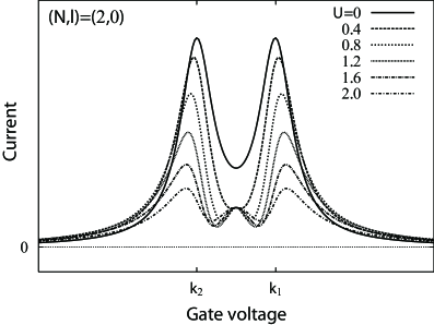
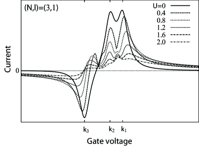
Figure 1: The current expectation value $\langle I\rangle^{(\ell)}$ for the scattering states. We fixed $t=1$.

We find resonance peaks in the vicinity of $\epsilon_{d}=(k_{i}+k_{j})/2$, which correspond to many-body scattering; they appear only for $U>0$. As is stressed above, the resonance of many-body scattering is originated from the phase shifts which are different for each two-body scattering in the lead $e$, in the lead $o$ and between the two leads. We also find resonance peaks in the vicinity of $\epsilon_{d}=k_{i}$, which correspond to one-body scattering at the quantum dot and are reduced to Lorentzian peaks in the limit $U\to 0$. The resonance peaks in the vicinity of $\epsilon_{d}=(k_{i}+k_{j})/2$ were not present in Mehta and Andrei’s result [8]; their results are equal to the limit $U\to 0$ of our result. This is because the interaction effect would be canceled in the current expectation value $\langle I\rangle$ if we adopted the same phase shifts for all the two-body scattering in the lead $e$, in the lead $o$ and between the two leads. Our choice (Resonance in an open quantum dot system with a Coulomb interaction: a Bethe-ansatz approach) of the phase shifts of two-body scattering is more plausible in the context of eigenstates as mentioned above. It would be interesting to discuss how the resonance of many-body scattering affects the transport properties of the interacting open quantum system out of equilibrium.

References

• [1] N. Andrei, Phys. Rev. Lett. 45 (1980), 379.
• [2] N. Andrei, K. Furuya and J. H. Lowenstein, Rev. Mod. Phys. 55 (1983), 331.
• [3] V. M. Filyov and P. B. Wiegmann, Phys. Lett. A 76 (1980), 283.
• [4] A. M. Tsvelick and P. B. Wiegmann, Adv. Phys. 32 (1983), 453.
• [5] P. B. Wiegmann, Phys. Let. A 80 (1980), 163.
• [6] R. M. Konik, H. Saleur and A. Ludwig, Phys. Rev. B 66 (2002), 125304.
• [7] R. M. Konik, H. Saleur and A. W. W. Ludwig, Phys. Rev. Lett. 87 (2001), 236801.
• [8] P. Mehta and N. Andrei, Phys. Rev. Lett. 96 (2006), 216802.
• [9] S. M. Cronenwett, T. H. Oosterkamp and L. P. Kouwenhoven, Science 281 (1998), 540.
• [10] D. Goldhaber-Gordon, J. Gores, M. A. Kastner, H. Shtrikman, D. Mahalu and U. Meirav, Phys. Rev. Lett. 81 (1998), 5225.
• [11] D. Goldhaber-Gordon, H. Shtrikman, D. Mahalu, D. Abusch-Magder, U. Meirav and M. A. Kastner, Nature (London) 391 (1998), 156.
• [12] D. C. Ralph and R. A. Buhrman, Phys. Rev. Lett. 69 (1992), 2118.
• [13] D. C. Ralph and R. A. Buhrman, Phys. Rev. Lett. 72 (1994), 3401.
• [14] Y. Meir, N. S. Wingreen and P. A. Lee, Phys. Rev. Lett. 66 (1991), 3048.
• [15] A. Levy Yeyati, A. Martin-Rodero and F. Flores, Phys. Rev. Lett. 71 (1993), 2991.
• [16] S. Datta, Electronic Transport in Mesoscopic Systems (Cambridge University, Cambridge, England, 1995).
• [17] A. M. Zagoskin, Quantum Theory of Many-Body Systems, Graduate Texts in Contemporary Physics (Springer, New York, 1998).
• [18] A. Schiller and S. Hershfield, Phys. Rev. B 58 (1998), 14978.