Comparing Star Formation on Large Scales in the c2d Legacy Clouds: Bolocam 1.1 mm Dust Continuum Surveys of Serpens, Perseus, and Ophiuchus
Abstract
We have undertaken an unprecedentedly large 1.1 millimeter continuum survey of three nearby star forming clouds using Bolocam at the Caltech Submillimeter Observatory. We mapped the largest areas in each cloud at millimeter or submillimeter wavelengths to date: 7.5 deg2 in Perseus (Paper I), 10.8 deg2 in Ophiuchus (Paper II), and 1.5 deg2 in Serpens with a resolution of 31″, detecting 122, 44, and 35 cores, respectively. Here we report on results of the Serpens survey and compare the three clouds. Average measured angular core sizes and their dependence on resolution suggest that many of the observed sources are consistent with power-law density profiles. Tests of the effects of cloud distance reveal that linear resolution strongly affects measured source sizes and densities, but not the shape of the mass distribution. Core mass distribution slopes in Perseus and Ophiuchus ( and ) are consistent with recent measurements of the stellar IMF, whereas the Serpens distribution is flatter (). We also compare the relative mass distribution shapes to predictions from turbulent fragmentation simulations. Dense cores constitute less than 10% of the total cloud mass in all three clouds, consistent with other measurements of low star-formation efficiencies. Furthermore, most cores are found at high column densities; more than 75% of 1.1 mm cores are associated with mag in Perseus, 15 mag in Serpens, and mag in Ophiuchus.
Subject headings:
stars: formation — ISM: clouds — ISM: individual (Serpens, Perseus, Ophiuchus) — submillimeter1. Introduction
Large-scale physical conditions in molecular clouds influence the outcome of local star formation, including the stellar initial mass function, star-formation efficiency, and the spatial distribution of stars within clouds (e.g. Evans, 1999). The physical processes that provide support of molecular clouds and control the fragmentation of cloud material into star-forming cores remain a matter of debate. In the classical picture magnetic fields provide support and collapse occurs via ambipolar diffusion (e.g. Shu et al., 1978), but many simulations now suggest that turbulence dominates both support and fragmentation (for a review see Mac Low & Klessen, 2004).
Dense prestellar and protostellar condensations, or cores (for definitions and an overview see Di Francesco et al., 2005), provide a crucial link between the global processes that control star formation on large scales and the properties of newly-formed stars. The mass and spatial distributions of such cores retain imprints of the fragmentation process, prior to significant influence from later protostellar stages such as mass ejection in outflows, core dissipation, and dynamical interactions. These cold (10 K), dense ( cm-3) cores are most easily observed at millimeter and submillimeter wavelengths where continuum emission from cold dust becomes optically thin and traces the total mass. Thus, complete maps of molecular clouds at millimeter wavelengths are important for addressing some of the outstanding questions in star formation.
Recent advances in millimeter and submillimeter wavelength continuum detectors have enabled a number of large-scale surveys of nearby molecular clouds (e.g. Johnstone et al., 2004; Kirk et al., 2005; Hatchell et al., 2005; Enoch et al., 2006; Stanke et al., 2006; Young et al., 2006). In addition to tracing the current and future star-forming activity of the clouds on large scales, millimeter and submillimeter observations are essential to understanding the properties of starless cores and the envelopes of the most deeply embedded protostars (for more on the utility of millimeter observations, see Enoch et al., 2006).
We have recently completed 1.1 mm surveys of Perseus (Enoch et al., 2006, hereafter Paper I) and Ophiuchus (Young et al., 2006, hereafter Paper II) with Bolocam at the Caltech Submillimeter Observatory (CSO). In this work we present a similar 1.1 mm survey of Serpens, completing our three-cloud study of nearby northern star-forming molecular clouds. Unlike previous work, our surveys not only cover the largest area in each cloud to date, but the uniform instrumental properties allow a comprehensive comparison of the cloud environments in these three regions. A comparison of the results for all three clouds provides insights into global cloud conditions and highlights the influence that cloud environment has on properties of star forming cores.
Background facts on the Perseus and Ophiuchus molecular clouds are discussed in Papers I and II. The Serpens molecular cloud is an active star formation region at a distance of pc (Straizys et al., 1996). Although the cloud extends more then 10 deg2 as mapped by optical extinction (Cambrésy, 1999), most observations of the region have been focused near the main Serpens cluster at a Right Ascension (R.A.) of and declination (decl.) of (J2000).
The Serpens cluster is a highly extincted region with a high density of young stellar objects (YSOs), including a number of Class 0 protostars. It has been studied extensively at near-infrared, far-infrared, submillimeter, and millimeter wavelengths (e.g. Eiroa & Casali, 1992; Hurt & Barsony, 1996; Larsson et al., 2000; Davis et al., 1999; Casali, Eiroa, & Duncan, 1993; Testi & Sargent, 1998). Some recent work has also drawn attention to a less well known cluster to the south, sometimes referred to as Serpens/G3-G6 (Djupvik et al., 2006; Harvey et al., 2006). Beyond these two clusters no continuum millimeter or submillimeter continuum surveys have been done that could shed light on large-scale star formation processes.
Following Papers I and II, we utilize the wide-field mapping capabilities of Bolocam, a large format bolometer array at the CSO, to complete millimeter continuum observations of 1.5 deg2 of the Serpens cloud. These observations are coordinated to cover the area mapped with Spitzer Space Telescope IRAC and MIPS observations of Serpens from the “Cores to Disks” (c2d Evans et al., 2003) legacy project. While millimeter and submillimeter observations are essential to understanding the properties of dense prestellar cores and protostellar envelopes, infrared observations are necessary to characterize the protostars embedded within those envelopes. In a future paper (M. Enoch et al. 2007, in preparation) we will take advantage of the overlap between our 1.1 mm maps and the c2d Spitzer Legacy maps to characterize the deeply embedded and prestellar populations in Serpens.
Here the Bolocam observations and data reduction (§ 2), general cloud morphology and source properties (§ 3), and summary (§ 4) for Serpens are briefly presented. In § 5 we compare the millimeter survey results for Serpens, Perseus, and Ophiuchus. First, we outline our operational definition of a millimeter core including instrumental effects in § 5.1, and discuss the observational biases introduced by different cloud distances in § 5.2. Physical implications of source sizes and shapes, and differences between the clouds, are discussed in § 5.3. We examine source densities and compare the cloud mass versus size distributions in § 5.4. We analyze the core mass distributions and their relation to cloud turbulence in § 5.5, and the spatial distributions of the core samples and clustering in § 5.6. The relationship of dense cores to the surrounding cloud column density and the mass fraction in dense cores are discussed in § 5.7 and § 5.8. We end with a summary in § 6.
2. Serpens Observations and Data Reduction
Observations and data reduction for Serpens follow the same methodology as for Perseus (Paper I) and Ophiuchus (Paper II). The data reduction techniques we have developed for the molecular cloud data are described in detail in Paper I and Paper II, including removal of sky noise, construction of pointing and calibration models, application of iterative mapping, and source extraction. Given these previous descriptions, only details specific to Serpens will be presented here. Further information about the Bolocam instrument and reduction pipeline is also available in Laurent et al. (2005).
2.1. Observations
As for Perseus and Ophiuchus, millimeter continuum observations of Serpens were made with Bolocam111http://www.cso.caltech.edu/bolocam at the CSO on Mauna Kea, Hawaii. Bolocam is a 144-element bolometer array that operates at millimeter wavelengths and is designed to map large fields (Glenn et al., 2003). Observations of Serpens were carried out at a wavelength of mm, where the field of view is and the beam is well approximated by a Gaussian with full-width at half-maximum (FWHM) size of 31. The instrument has a bandwidth of 45 GHz at mm, excluding the CO (J=2-1) line to approximately 99%.
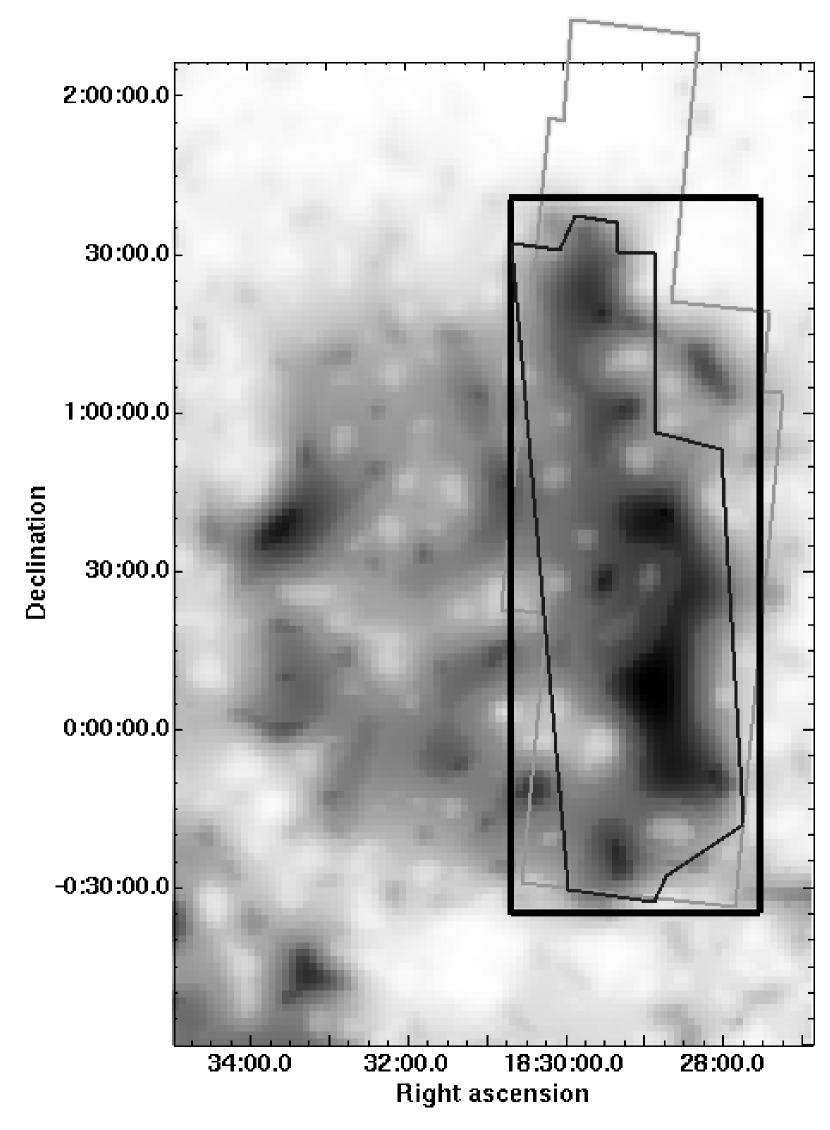
The 1.1mm observations were designed to cover a region with magnitudes () in the visual extinction map of Cambrésy (1999), shown in Figure 1. As demonstrated in Figure 1, this ensures that the Bolocam observations overlap as closely as possible with the region of Serpens observed with Spitzer IRAC and MIPS as part of the c2d Legacy project. In practice, the Bolocam survey covers a region slightly larger than the IRAC map, and slightly smaller than the MIPS map.
Serpens was observed during two separate runs in 2003 May 21-June 9 and 2005 June 26-30. During the 2003 run, 94 of the 144 channels were operational, compared to 109 during the 2005 run. Scans of Serpens were made at a rate of sec-1 with no chopping of the secondary. The final map consists of 13 scans from 2003 in good weather, and 17 scans from 2005 in somewhat poorer conditions. Each scan covered the entire 1.5 deg2 area and took minutes to complete depending on the scan direction. Scans were made in two orthogonal directions, approximately half in R.A. and half in decl. This strategy allows for good cross-linking in the final map, sub-Nyquist sampling, and minimal striping from noise. Scans were observed in sets of three offset by , , to optimize coverage.
In addition, small maps of pointing sources were observed approximately every 2 hours, and at least one primary flux calibration source, including Neptune, Uranus, and Mars, was observed each night. Several larger beam maps of planets were also made during each run, to characterize the Bolocam beam at 1.1 mm.
2.2. Pointing and Flux Calibration
A pointing model for Serpens was generated using two nearby pointing sources, G 34.3 and the quasar 1749+096. After application of the pointing model, a comparison to the literature SCUBA positions of four bright known sources (Davis et al., 1999) in the main Serpens cluster indicated a constant positional offset of (R.A., decl.) = (5, ). We corrected for the positional offset, but estimate an uncertainty in the absolute pointing of , still small compared to the beam size of 31″. The relative pointing errors, which cause blurring of sources and an increase in the effective beam size, should be much smaller, approximately . Relative pointing errors are characterized by the rms pointing uncertainty, derived from the deviations of G 34.3 from the pointing model.
The Bolocam flux calibration method makes real-time corrections for the atmospheric attenuation and bolometer operating point using the bolometer optical loading, by calculating the calibration factor as a function of the bolometer DC resistence. Calibrator maps of Neptune, Uranus, and G 34.3, observed at least once per night, were used to construct a calibration curve for each run. A systematic uncertainty of approximately 10% is associated with the absolute flux calibration, but relative fluxes should be much more accurate.
2.3. Cleaning and Iterative mapping
Aggressive sky subtraction techniques are required for Bolocam data to remove sky noise, which dominates over the astronomical signal before cleaning. As in Papers I and II, we remove sky noise from the Serpens scans using Principal Component Analysis (PCA) cleaning (Laurent et al. (2005) and references therein), by subtracting 3 PCA components.
As described in Paper I, PCA cleaning removes some source flux from the map as well as sky noise, necessitating the use of an iterative mapping procedure to recover lost astronomical flux. In this procedure, sky subtraction is refined by iteratively removing a source model (derived from the cleaned map) from the raw data, thereby reducing contamination of the sky template by bright sources. Simulations show that at least 98% of source flux density is recovered after 5 iterations, with the exception of very large ( FWHM) faint sources, for which we only recover 90% or less of the true flux density (See Paper I). We conservatively estimate a 10% residual photometric uncertainty from sky subtraction after iterative mapping, in addition to the 10% uncertainty in the absolute flux calibration.
Data from the 2003 and 2005 observing runs were iteratively mapped separately because they required different pointing and flux calibration models. After iterative mapping the two epochs were averaged, weighted by the square root of the observational coverage.
2.4. Source Identification
Millimeter cores are identified in an optimally filtered map using the source extraction method described in Paper I. Because the signal from a point source lies in a limited frequency band, we can use an optimal (Wiener) filter in Fourier space to attenuate noise at low frequencies, as well as high frequency noise above the signal band. The optimal filter preserves the resolution of the map and the peak brightness of point sources but reduces the rms noise per pixel by approximately , thereby optimizing the source signal-to-noise (S/N). Extended sources will have slightly enhanced peak values in the optimally filtered map. After optimal filtering, the map is trimmed to remove areas of low coverage. Note that the optimally filtered map is used for source detection only; all photometry is measured in the unfiltered map, and all maps displayed here are unfiltered.
Observational coverage, which depends on the scan strategy, number of scans, and number of bolometer channels, was very uniform for Serpens; trimming regions where the coverage was less than 30% of the peak coverage was equivalent to cutting off the noisy outer edges of the map. The average coverage of the Serpens map is 1600 hits per pixel, where a hit means a bolometer passed over this position, with differences in hits per pixel across the map of 18%. The average coverage corresponds to an integration time of 13 minutes per pixel, although individual pixels are not independent because the map is over-sampled.
For each pixel, the local rms noise is calculated in small (45 arcmin2) boxes using a noise map from which sources have been removed. This noise map is derived as part of the iterative mapping process (see Paper I). A simple peak-finding routine identifies all pixels in the optimally filtered map more than above the local rms noise level, and source positions are determined using an IDL centroiding routine. Each new source must be separated by at least a beam size from any previously identified source centroid. The centroid is a weighted average position based on the surface brightness within a specified aperture, and is computed as the position at which the derivatives of the partial sums of the input image over (y,x) with respect to (x,y) equal zero. A given centroid is considered “well defined” as long as the computed derivatives are decreasing. All sources were additionally inspected by eye to remove spurious peaks near the noisier edges of the map.
3. Serpens Results
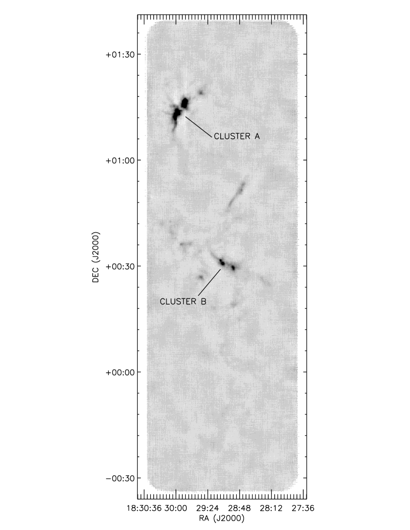
The final pixel-1 Serpens map is shown in Figure 2, with the well known northern Serpens cluster, Cluster A (Harvey et al., 2006), indicated, as well as the southern cluster, Cluster B (Serpens/G3-G6). Covering a total area of 1.5 deg2, or 30.9 pc2 at a distance of 260 pc, the map has a linear resolution of AU.
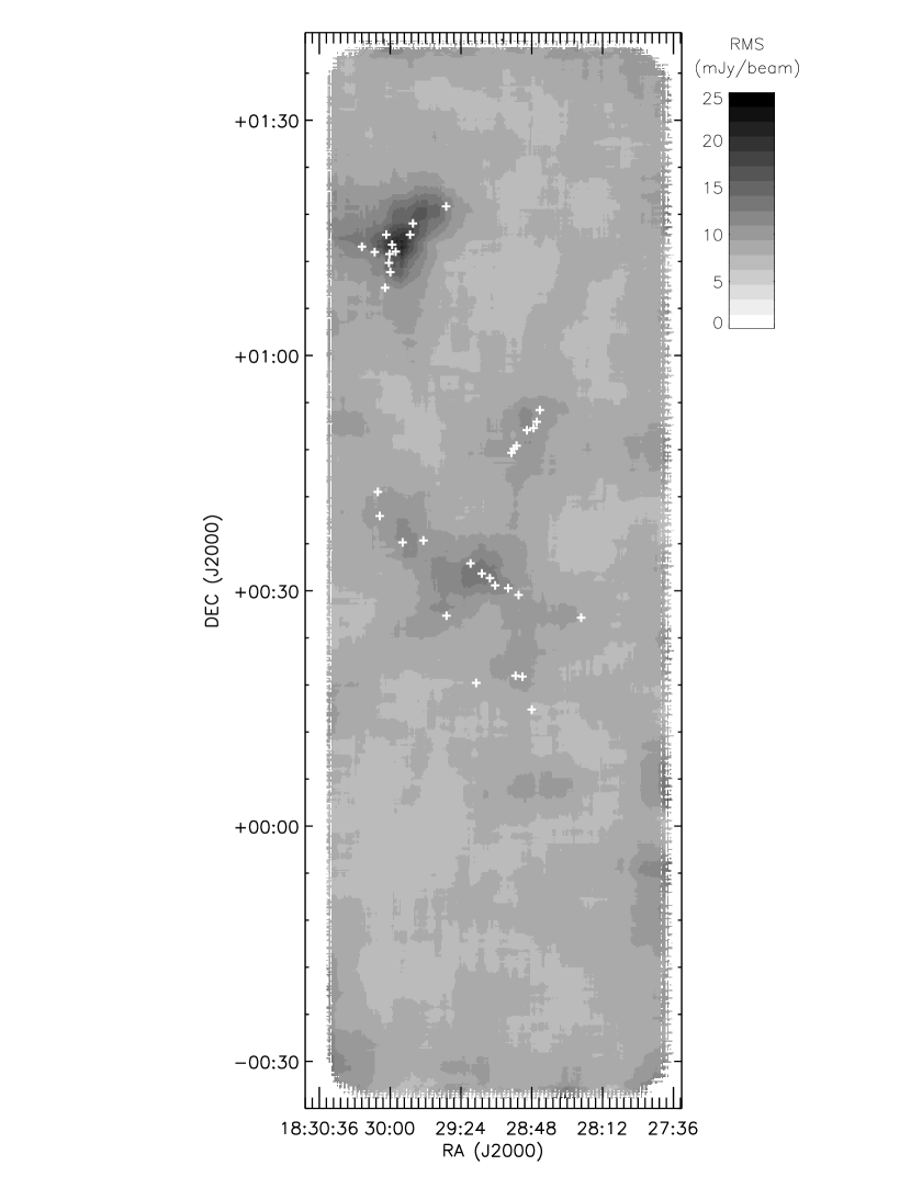
We identify 35 sources above the detection limit in the Serpens map. The limit is based on the local rms noise, and is typically 50 mJy beam-1. The noise map for Serpens is shown in Figure 3, with the positions of identified sources overlaid. The mean rms noise is 9.5 mJy beam-1, but is higher near bright sources. Most of the 18% variations in the local rms noise occur in the main cluster region, where calculation of the noise is confused by residual artifacts from bright sources. Such artifacts must contribute significantly to noise fluctuations; coverage variations alone would predict rms noise variations of only . This means that faint sources near bright regions have a slightly lower chance of being detected than those in isolation.
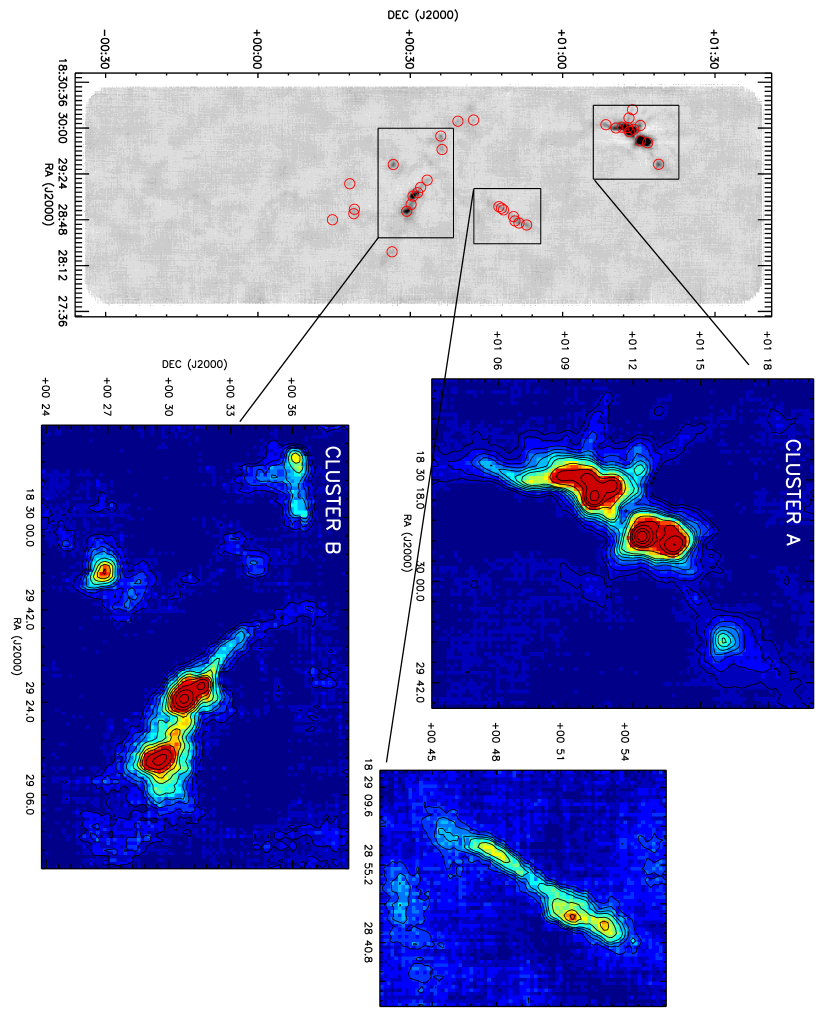
Source positions are listed in Table 1, and identified by red circles in Figure 4. Figure 4 also shows magnifications of the more densely populated source regions, including Cluster A and Cluster B. We do not see any circularly symmetric extended emission on scales in the map. It should, in principle, be possible to recover symmetric structures up to the array size of , but our simulations show that sources in size are severely affected by cleaning and therefore difficult to fully recover with iterative mapping. The map does contain larger filamentary structures up to long. In particular, the long filament between Cluster A and Cluster B is reminiscent of the elongated ridge near B1 in Perseus (Paper I). The Serpens filament does not contain the bright compact sources at either end that are seen in the B1 ridge, however.
Previous millimeter-wavelength maps of Cluster A, such as the 1.1 mm UKT14 map of Casali, Eiroa, & Duncan (1993) and the SCUBA map of Davis et al. (1999), generally agree with our results in terms of morphology and source structure. Not all of the individual sources are detected by our peak finding routine, presumably due to the poorer resolution of Bolocam () compared to SCUBA (), but most can, in fact, be identified by eye in the Bolocam map. An IRAM 1.3 mm continuum map of Cluster B with 11″ resolution (Djupvik et al., 2006) is visually quite similar to our Bolocam map of the region. We detect each of the four 1.3 mm sources identified (MMS1-4), although the 1.3 mm triplet MMS1 is seen as a single extended source in our map.
Most of the brightest cores, in particular those in Cluster A, are associated with known YSOs including a number of Class 0 objects (Hurt & Barsony, 1996; Harvey et al., 2006). All bright 1.1 mm sources are aligned with bright emission in the Spitzer MIPS map of Serpens observed by the c2d legacy project (Harvey et al., 2007). Fainter millimeter sources are usually associated with extended filaments, but do not necessarily correspond to point sources in the MIPS map. Conversely, one bright extended region of emission just south of Cluster A contains no 1.1 mm sources. This area also exhibits extended emission at 70 and 24 , which may be indicative of warmer, more diffuse material than that of the dense cores detected at 1.1 mm.
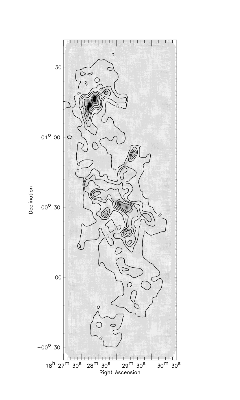
Despite the low rms noise level achieved in Serpens, very few sources are seen outside the main clusters; most of the area that we mapped appears devoid of 1.1 mm emission, despite being in a region of high extinction. Figure 5 shows a comparison between the Bolocam millimeter map (gray-scale) and visual extinction (contours) derived from c2d near- and mid-infrared Spitzer data.
The majority of sources (90–95%) detected by IRAC and MIPS in the c2d clouds have spectral energy distributions characteristic of reddened stars. Thus we have measures of the visual extinction for many lines of sight through the molecular clouds imaged by c2d. Line-of-sight extinction values are derived by fitting the RV=5.5 dust model of Weingartner & Draine (2001) to the near-infrared through mid-infrared SED (Evans et al., 2006). For each of the three clouds, the derived line-of-sight extinctions were convolved with uniformly spaced 90″ Gaussian beams to construct an extinction map.
Extinction maps used throughout this paper for Serpens, Perseus, and Ophiuchus are derived from c2d data by this method. The c2d extinction maps accurately trace column densities up to , but are relatively insensitive to small regions of high volume density, because they rely on the detection of background stars. Thus the extinction maps are complementary to the 1.1 mm observations, which trace high volume density structures (see § 5.1). In Figure 5, the map for Serpens is smoothed to an effective resolution of .
As can be seen in Figure 5, nearly all Serpens millimeter sources lie within regions of high visual extinction () and, in particular, all bright Bolocam sources are associated with areas of . Nevertheless, there are a number of high extinction areas () with no detectable 1.1 mm sources. A similar general trend was noted in both Perseus (Paper I) and Ophiuchus (Paper II), with relatively few sources found outside the major groups and clusters associated with the highest extinction. § 5.7 examines the relationship between and 1.1 mm sources in more detail.
3.1. Source Properties
3.1.1 Positions and Photometry
Positions, peak flux densities, and S/N for the 35 1.1 mm sources identified in the Bolocam map of Serpens are listed in Table 1. The S/N ratio is measured in the optimally filtered map, whereas photometry and all other source properties are measured in the unfiltered, surface brightness normalized map. The peak flux density per beam () is given in mJy beam-1 (1 mJy beam MJy sr-1). Uncertainties in photometry are calculated from the local rms beam-1, calculated as in § 2.4. An additional systematic error of 15% is associated with all flux densities, from the absolute calibration uncertainty and the systematic bias remaining after iterative mapping. Table 1 also lists the most commonly used name from the literature for known sources, and indicates if the 1.1 mm source is coincident (within ) with a MIPS source from the c2d database (Harvey et al., 2007).
Table 2 lists photometry in fixed apertures of diameter , , and , and the total integrated flux density (). Integrated flux densities are measured assuming a sky value of zero, and include a correction for the Gaussian beam so that a point source has the same integrated flux density in all apertures. No integrated flux density is given if the distance to the nearest neighboring source is smaller than the aperture diameter. The total flux density is integrated in the largest aperture ( diameters in steps of ) that is smaller than the distance to the nearest neighboring source. Uncertainties are , where is the local rms beam-1 and (, ) are the aperture and beam FWHM respectively.
Peak and total flux density distributions for the 35 1.1 mm sources in Serpens are shown in Figure 6, with the detection limit indicated. In general, source total flux densities are larger than peak flux densities because most sources in the map are extended, with sizes larger than the beam. Both distributions look bimodal; all of the sources in the brighter peak are in either Cluster A or Cluster B. The mean peak flux density of the sample is 0.5 Jy beam-1, and the mean total flux density is 1.0 Jy, both with large standard deviations of order the mean value. Peak values of the cores, calculated from the peak flux density as in § 3.1.3, are indicated on the upper axis.
3.1.2 Sizes and Shapes
Source FWHM sizes and position angles (PA, measured east of north) are measured by fitting an elliptical Gaussian after masking out nearby sources using a mask radius equal to half the distance to the nearest neighbor. The best fit major and minor axis sizes and PAs are listed in Table 2. Errors given are the formal fitting errors and do not include uncertainties due to residual cleaning effects, which are of order for the FWHM and for the PA (see Paper I).
As can be seen in Figure 7, the minor axis FWHM values are fairly narrowly distributed around the sample mean of , with a standard deviation of . The major axis FWHM have a similarly narrow distribution with a mean of and a scatter of . On average sources are slightly elongated, with a mean axis ratio at the half-max contour (major axis FWHM / minor axis FWHM) of 1.3.
A morphology keyword for each source is also given in Table 2, to describe the general source shape and environment. Keywords indicate if the source is multiple (within of another source), extended (major axis full-width at ), elongated (axis ratio at ), round (axis ratio at ), or weak (peak flux densities less than 5 times the rms per pixel in the unfiltered map). The majority (28/35) of sources are multiple by this definition, and nearly all (32/35) are extended at the contour.
3.1.3 Masses, Densities, and Extinctions
The total mass of gas and dust in a core is proportional to the total flux density , assuming the dust emission at 1.1 mm is optically thin and both the dust temperature and opacity are independent of position within a core:
| (1) |
where cm2 g-1 is the dust opacity per gram of gas, pc is the distance, and K is the dust temperature. A gas to dust mass ratio of 100 is included in . The dust opacity is interpolated from Ossenkopf & Henning (1994, Table 1 column 5), for dust grains with thin ice mantles, coagulated for years at a gas density of cm-3. This opacity has been found to be the best fit in a number of radiative transfer models (Evans et al., 2001; Shirley et al., 2002; Young et al., 2003).
Masses calculated in this manner, assuming a dust temperature of K for all sources, are listed in Table 2. Uncertainties given are from the uncertainty in the total flux density only; additional uncertainties from , , and together introduce a total uncertainty in the mass of up to a factor of 4 or more (also see Paper I). The dust opacity is uncertain by up to a factor of two or more (Ossenkopf & Henning, 1994), owing to large uncertainties in the assumed dust properties, and possible positional variations of within a core. Variations in both and the cloud distance have smaller effects than dust temperature uncertainties for the range of plausible values ( cm2 g-1; pc; ).
Assuming K is a reasonable compromise to cover both prestellar and protostellar sources, based on the results of more detailed radiative transfer models (Evans et al., 2001; Shirley et al., 2002, see also discussion in Paper I). A temperature of 10 K will result in overestimates of the masses of protostellar cores, which will be warmer on the inside, by up to a factor of three (for a 20 K source). Temperature errors are not as problematic as they might seem, however, as most of the envelope mass is located at large radii and low temperatures (see also Paper I).
The total mass of the 35 1.1 mm cores in Serpens is , which is only 2.7% of the total cloud mass (3470 M⊙). The cloud mass is estimated from the c2d visual extinction map using H mag cm-2 (Bohlin et al., 1978) and
| (2) |
where is the distance, is the solid angle, indicates summation over all pixels in the extinction map, and is the mean molecular weight per H2 molecule.
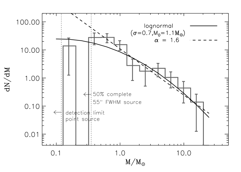
Figure 8 shows the differential mass function of all 1.1 mm sources in Serpens. The point source detection limit of is indicated, as well as the 50% completeness limit for sources of FWHM 55 (), which is the average size of the sample. Completeness is determined from Monte Carlo simulations of simulated sources inserted into the raw data and run through the reduction pipeline, as described in Paper I. The best fit power law slope to is shown (), as well as the best fit lognormal slope.
Our mass distribution has a flatter slope than that found by Testi & Sargent (1998) from higher resolution () OVRO observations ( for ). This may be due in part to the fact that most of our detections, at least 25/35, lie outside the area observed by Testi & Sargent (1998). The resolution differences of the observations may also contribute significantly; for example, a number of our bright sources break down into multiple objects in the resolution map.
From the peak flux density we calculate the central H2 column density for each source:
| (3) |
Here is the beam solid angle, is the mass of hydrogen, cm2g-1 is the dust opacity per gram of gas, is the Planck function, =10 K is the dust temperature, and as above. From column density we convert to extinction: H mag cm-2 (Bohlin et al., 1978), adopting . We note, however, that this relation was determined for the diffuse interstellar medium and may not be ideal for the highly extincted lines of sight probed here.
The resulting peak values are listed in Table 2. The average peak of the sample is 41m with a large standard deviation of 55m and a maximum of 256m. Extinctions calculated from the millimeter emission are generally higher than those from the c2d visual extinction map by approximately a factor of 7, likely a combination of both the higher resolution of the Bolocam map ( compared with ) and the fact that the extinction map cannot trace the highest volume densities because it relies on the detection of background sources. Grain growth in dense cores beyond that included in the dust opacity from Ossenkopf & Henning (1994) could also lead to an overestimate of the from out 1.1 mm data.
Also listed in Table 2 is the mean particle density:
| (4) |
where is the total mass, is the linear deconvolved half-width at half-max size, and is the mean molecular weight per particle. The median of the source mean densities is cm-3, with values ranging from to cm-3.
4. Serpens Summary
We have completed a 1.1 mm dust continuum survey of Serpens, covering deg2, with Bolocam at the CSO. We identify 35 1.1 mm sources in Serpens above a detection limit which is 50 mJy beam-1, or , on average. The sample has an average mass of , and an average source FWHM size of . On average, sources are slightly elongated with a mean axis ratio at half-max of 1.3. The differential mass distribution of all 35 cores is consistent with a power law of slope above . The total mass in dense 1.1 mm cores in Serpens is , accounting for 2.7% of the total cloud mass, as estimated from our c2d visual extinction map.
5. Three-Cloud Comparison of Perseus, Ophiuchus, and Serpens
The survey of Serpens completes a three-cloud study investigating the properties of millimeter emission in nearby star-forming molecular clouds: Perseus (Enoch et al., 2006), Ophiuchus (Young et al., 2006), and Serpens. Having presented the results for the Serpens cloud, we now compare the three clouds.
Our large-scale millimeter surveys of Perseus, Ophiuchus, and Serpens, completed with the same instrument and reduction techniques, provide us with a unique basis for comparing the properties of 1.1 mm emission in a variety of star-forming environments. In the following sections we examine similarities and differences in the samples of star-forming cores, and discuss implications for physical properties of cores as well as global cloud conditions.
5.1. What is a core?
Before comparing results from the three clouds, we first describe our operational definition of a millimeter core. The response of Bolocam to extended emission, together with observed sensitivity limits determine the type of structure that is detectable in our 1.1 mm maps The Bolocam 1.1 mm observations presented here are sensitive to sub-structures in molecular clouds with volume density cm-3. One way to see this is to calculate the mean density along the curve defined by the detection as a function of size in each cloud.
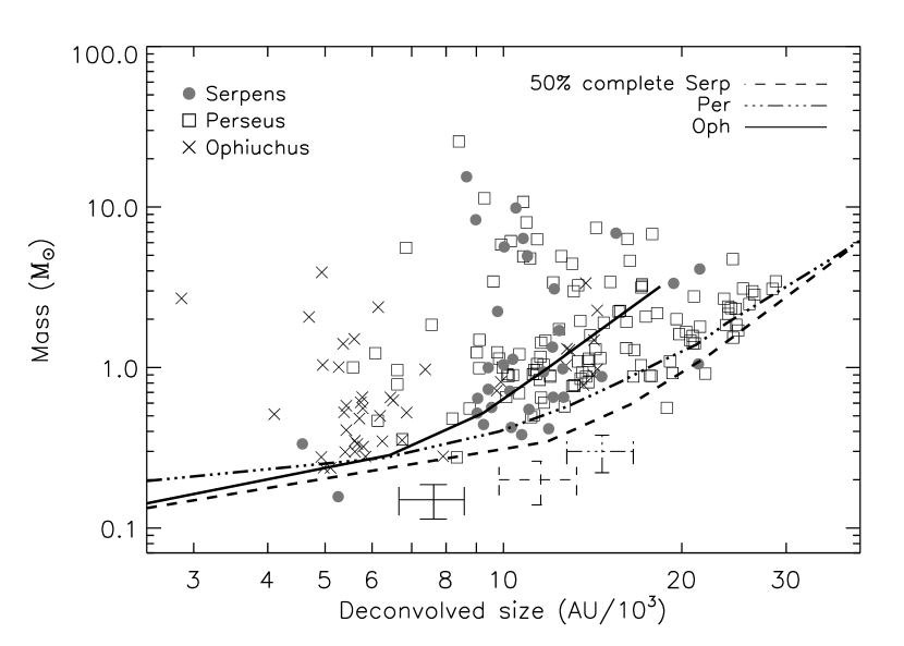
Figure 9 demonstrates how the completeness in each cloud varies as a function of source size. Plotted symbols give the total mass versus linear deconvolved size for all sources detected in each cloud, and lines indicate the empirically derived 50% completeness limits. For Ophiuchus the average completeness curve is plotted; as the rms noise varies considerably in Ophiuchus, some regions have higher or lower completeness limits than the curve shown here. Completeness is determined from Monte Carlo simulations by adding simulated sources to the raw data, processing them in the same way as the real data, and attempting to detect them using our peak-finding algorithm (see Paper I). We are biased against detecting large diffuse sources because we detect sources based on their peak flux density, whereas the mass is calculated from the total flux, which scales approximately as the size squared.
Calculating mean densities along the 50% completeness curve in each cloud yields cm-3 in Serpens, cm-3 in Perseus, and cm-3 in Ophiuchus. By comparison, the mean cloud density as probed by the extinction map is approximately 1000 cm-3 in Serpens, 220 cm-3 in Perseus, and 390 cm-3 in Ophiuchus. To be identified as a core, therefore, individual structures must have a mean density cm-3, and a contrast compared to the average background density of at least 30-100. The mean cloud density is estimated from the total cloud mass (§ 3.1.3) and assumes a cloud volume of , where A is the area of the extinction map within the contour.
Although we are primarily sensitive to cores with high density contrast compared to the background, it is clear that there is structure in the 1.1 mm map at lower contrasts as well, and that many cores are embedded within lower density filaments. The total mass in each of the 1.1 mm maps, calculated from the sum of all pixels , is approximately twice the mass in dense cores: 176M⊙ versus 92M⊙ in Serpens, 376M⊙ versus 278M⊙ in Perseus, and 83M⊙ versus 44M⊙ in Ophiuchus, for ratios of total 1.1 mm mass to total core mass of 1.9, 1.4, and 1.9 respectively. Thus about half the mass detectable at 1.1 mm is not contained in dense cores, but is rather in the “foothills” between high density cores and the lower density cloud medium.
Structures that meet the above sensitivity criteria and are identified by our peak-finding routine are considered cores. Our peak-finding method will cause extended filaments to be broken up into several separate “cores” if there are local maxima in the filament separated by more than one beam size, and if each has a well-defined centroid (see § 2.4). There is some question as to whether these objects should be considered separate sources or a single extended structure, but we believe that our method is more reliable for these data than alternative methods such as Clumpfind (Williams et al., 1994). In Paper I we found that faint extended sources in our maps, which one would consider single if examining by eye, are often partitioned into multiple sources by Clumpfind. Using our method, one filamentary structure in Serpens is broken up into several sources, as are two filaments in Perseus.
Monte Carlo tests were done to quantify biases and systematic errors introduced by the cleaning and iterative mapping process, which affect the kind of structure we can detect. Measured FWHM, axis ratios, and position angles are not significantly affected by either cleaning or iterative mapping for sources with FWHM; likewise, any loss of flux for such sources has an amplitude less than that of the rms noise. Sources with FWHM are detected, but with reduced flux density (by up to 50%), and large errors in the measured FWHM sizes of up to a factor of two.
The limitation on measurable core sizes of approximately corresponds to AU in Perseus and Serpens, and AU in Ophiuchus. Note that these sizes are of order the median core separation in each cloud (see § 5.6), meaning that we are just as likely to be limited by the crowding of cores as by our sensitivity limits in the measurement of large cores. The dependence of measurable core size on cloud distance can be seen in Figure 9, where the completeness rises steeply at smaller linear deconvolved sizes for Ophiuchus than for Perseus or Serpens. Thus we are biased against measuring large cores in Ophiuchus compared to the other two clouds. Although there are cores in our sample with sizes up to AU (Figure 9), most cores have sizes substantially smaller than the largest measurable value, again indicating that we are not limited by systematics.
To summarize, the Bolocam 1.1 mm observations presented here naturally pick out sub-structures in molecular clouds with high volume density ( cm-3). These millimeter cores have a contrast of at least compared to the average cloud density as measured by the visual extinction map ( cm-3). Many cores are embedded in lower density extended structures, which contribute approximately half the mass measurable in the Bolocam 1.1 mm maps. Finally, Monte Carlo tests indicate that we can detect cores with intrinsic sizes up to approximately .
5.2. Distance effects
To test the effects of instrumental resolution and its dependence on distance, we convolve the Ophiuchus map with a larger beam to simulate putting it at approximately the same distance as Perseus and Serpens. After convolving the unfiltered Ophiuchus map to resolution, we apply the optimal filter and re-compute the local rms noise, as described for Serpens (§ 2.4). The pixel scale in the convolved map is still 10″ pixel-1, but the resolution is now and the rms is lower than in the original map, with a median value of 17 mJy beam-1 in the main L 1688 region. Source detection and photometry is carried out in the same way as for the original map, with the exception that a 62″ beam is assumed.
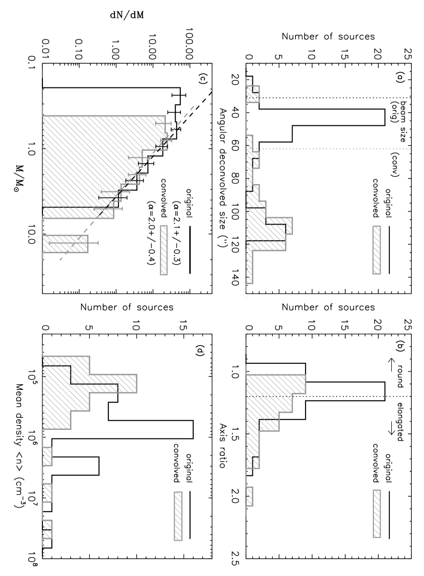
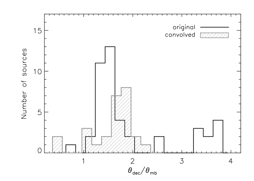
We detect 26 sources in the degraded-resolution map, or 40% fewer than the 44 sources in the original map. Therefore a number of sources do become confused at lower resolution. The basic source properties for the original and degraded-resolution samples, including angular deconvolved sizes, axis ratios, mass distribution, and mean densities, are compared in Figure 10. Here the angular deconvolved size is defined as , where is the geometric mean of the measured minor and major axis FWHM sizes and is the pointing-smeared beam FWHM ( and for the original and degraded resolution maps, respectively).
We note that the average source size in the degraded-resolution map is nearly twice that in the original Ophiuchus map (average angular deconvolved size of versus ). Such a large size difference cannot be fully accounted for by blending of sources, as even isolated sources show the same effect. This behavior provides clues to the intrinsic intensity profile of the sources. For example, a gaussian intensity profile or a solid disk of constant intensity will both have measured deconvolved sizes that are similar in maps with and beams. Conversely, a power law intensity profile will have a larger measured size in the resolution map.
The ratio of angular deconvolved size to beam size (; Figure 11) are similar for the degraded-resolution (median ) and original (median ) samples, further evidence for power law intensity profiles. An intrinsic gaussian or solid disk intensity profile will result in values in the degraded-resolution map that are approximately half those in the original map, while a intensity profile results in similar values in the degraded-resolution and original map (0.9 versus 1.3). We discuss source profiles further in Section 5.3 below.
Sources in the degraded-resolution map appear slightly more elongated, with an average axis ratio at the half-maximum contour of compared to for the original map. Larger axis ratios are expected for blended sources in a lower-resolution map. The slope of the mass distribution is not significantly changed: for the degraded-resolution sample compared to for the original sample. The factor of two increase in deconvolved sizes do create lower mean densities in the degraded-resolution sample, however (median density of cm-3 compared to cm-3 for the original sample). The effect of resolution on mean densities will be discussed further in § 5.4.
Given the small number of sources in the degraded-resolution map, we carry out the three cloud comparison below using the original Ophiuchus map to mitigate uncertainties from small number statistics. Any notable differences between the original and degraded-resolution Ophiuchus results will be discussed where appropriate.
5.3. Physical Implications of Source Sizes and Shapes
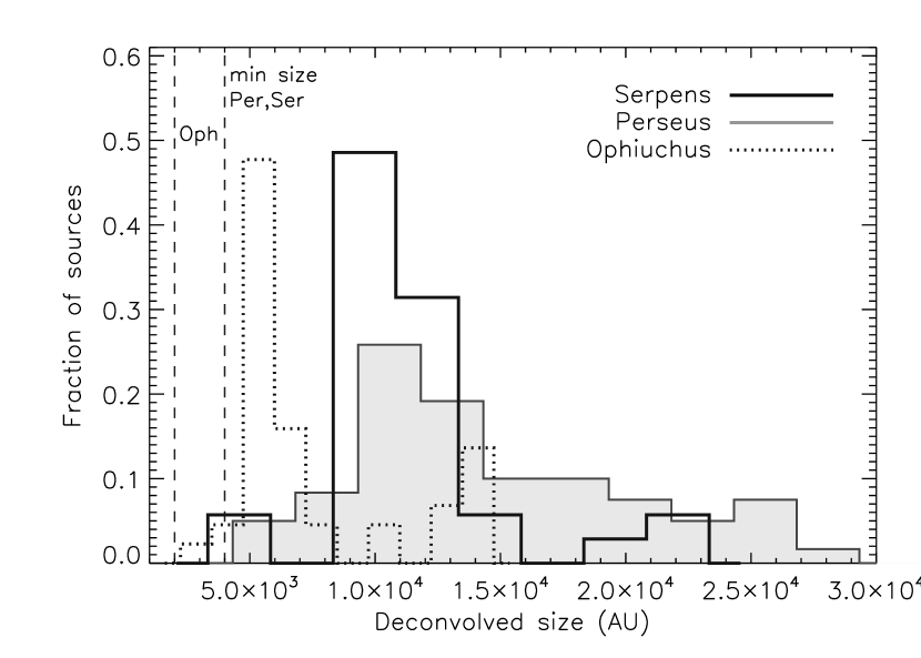
To compare sources in clouds at different distances, we first look at the linear deconvolved size: , where is the cloud distance, is measured angular size, and is the beam size. The distributions of linear deconvolved source sizes for the three clouds are shown in Figure 12, left. Sources in Ophiuchus have smaller deconvolved sizes than those in Perseus or Serpens by almost a factor of two, with mean vales of AU in Ophiuchus compared to AU in Serpens and AU in Perseus. There is a systematic uncertainty in the deconvolved size associated with the uncertainty in the effective beam size, which becomes larger with larger pointing errors. The effective beam in any of the three clouds may be as large as , which would decrease deconvolved sizes negligibly, by up to AU depending on the distance and measured size.
While there are possible physical explanations for intrinsic size differences, for instance a denser medium with a shorter Jeans length should produce smaller cores on average, we are more likely seeing a consequence of the higher linear resolution in Ophiuchus, as discussed in § 5.2. Thus cores in Serpens and Perseus would likely appear smaller if observed at higher resolution, and measured linear deconvolved sizes should be regarded as upper limits. To reduce the effects of distance, we examine the ratio of angular deconvolved size to beam size (; Figure 12, right). We found in § 5.2 that does not depend strongly on the linear resolution, but does depend on the intrinsic source intensity profile.
If the millimeter sources follow power law density distributions, which do not have a well defined size, then Young et al. (2003, hereafter Y03) show that depends on the index of the power-law, and not on the distance of the source. So, for example, if sources in Perseus and Ophiuchus have the same intrinsic power law profile, the mean should be similar in the two clouds, and the mean linear deconvolved size should be twice as small in Ophiuchus because it lies at half the distance. This is precisely the behavior we observe, suggesting that many of the detected 1.1 mm sources have power law density profiles.
Considering that a number of the 1.1 mm sources have internal luminosity sources (M. Enoch et al. 2007, in preparation), and that protostellar envelopes are often well described by power law profiles (Shirley et al., 2002, Y03), this is certainly a plausible scenario. According to the correlation between and density power law exponent found by Y03, median values of 1.7 in Perseus, 1.5 in Ophiuchus and 1.3 in Serpens would imply average indices of , 1.5, and 1.6 respectively. These numbers are consistent with mean values found from radiative transfer modeling of Class 0 and Class I envelopes (, Shirley et al., 2002, Y03), although the median for those samples is somewhat higher (). Note that source profiles could deviate from a power-law on scales much smaller than the beam size, or on scales larger than our size sensitivity () without affecting our conclusions.
Perseus displays the widest dispersion of angular sizes, ranging continuously from . By contrast, more than half the sources in Serpens and Ophiuchus are within of their respective mean values. Although there is a group of Ophiuchus sources at large sizes in Figure 12, note that the degraded-resolution Ophiuchus sample displays a very narrow range of sizes (Figure 11), similar to Serpens. The observed size range in Perseus would correspond to a wide range of power law indices, from very shallow () to that of a singular isothermal sphere (). A more likely possibility, however, is that sources with large do not follow power law density profiles.
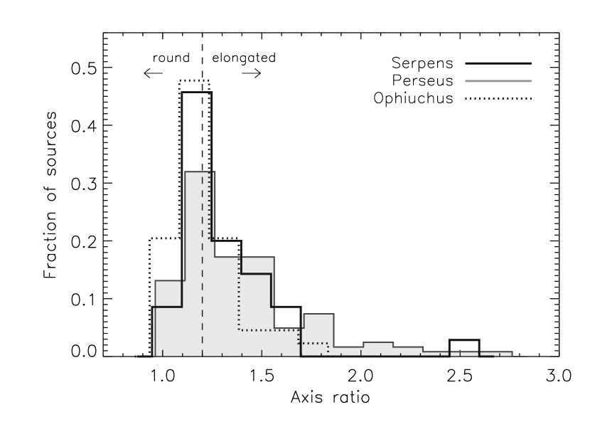
The axis ratio at the half-maximum contour is a simple measure of source shape. Figure 13 shows the distribution of 1.1 mm source axis ratios in the three clouds. Our simulations suggest that axis ratios of up to 1.2 can be introduced by the data reduction (Paper I), so we consider sources with an axis ratio to be round, and those with a ratio to be elongated. Sources in Ophiuchus tend to be round, with a mean axis ratio of 1.2, but note that the mean axis ratio in the degraded-resolution Ophiuchus sample is 1.3. The average axis ratio in Serpens is 1.3, and Perseus sources exhibit the largest axis ratios with a mean of 1.4 and a tail out to 2.7.
We found in Paper II that Ophiuchus sources were more elongated at the contour than at the half-max contour, as would be the case for round cores embedded in more elongated filaments. A similar situation is seen in Serpens; the average axis ratio at the contour is 1.4 in all three clouds. Thus cores in Perseus are somewhat elongated on average, while objects in Serpens and Ophiuchus appear more round at the half-max contour but elongated at the contour, suggesting round cores embedded in filamentary structures.
In addition to angular sizes, Y03 also note a relationship between axis ratio and density power law exponent, finding that aspherical sources are best modeled with shallower density profiles. The inverse proportionality between and axis ratio demonstrated in Figure 25 of Y03 suggests power law indices in all three clouds between 1.5 and 1.7. These values are consistent with those inferred from the average angular deconvolved source sizes, and the wider variation of axis ratios in Perseus again points to a larger range in for that cloud.
5.4. Densities and the Mass versus Size Distribution
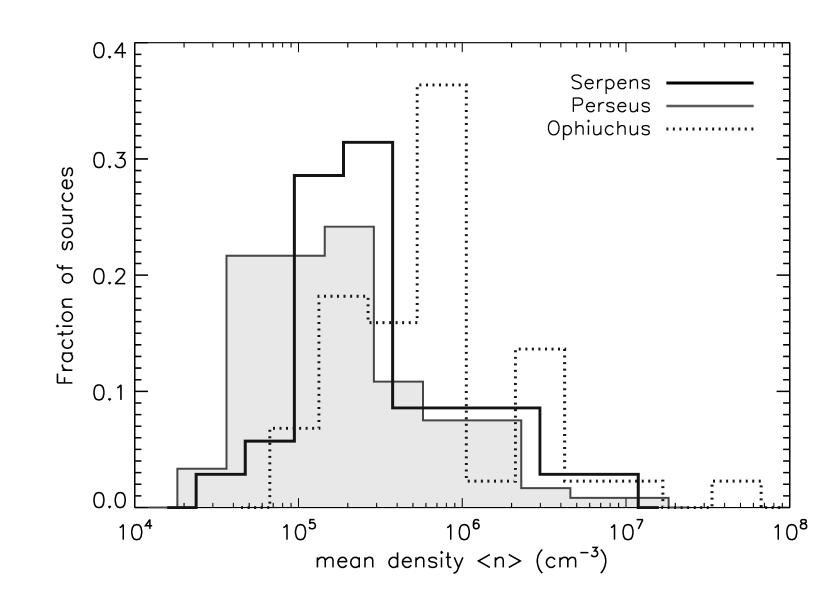
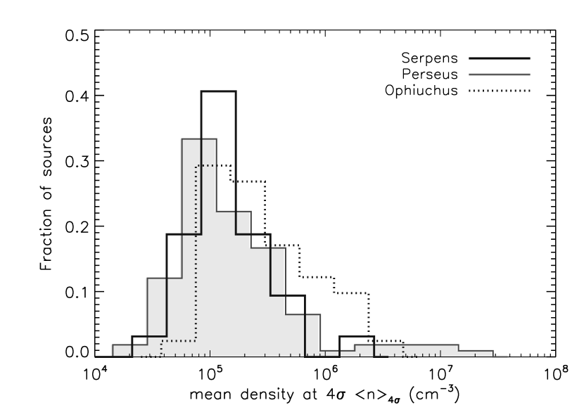
Mean densities calculated using linear deconvolved FWHM sizes appear to be significantly higher in Ophiuchus, where the median of the mean densities of the sample is cm-3, than in Serpens (median density cm-3) or Perseus (median density cm-3), as seen in Figure 14, left. There is a large scatter with standard deviation of order twice the mean value in all three clouds. Sources in Ophiuchus tend to be less massive than in the other two clouds, so the larger mean densities can be entirely attributed to smaller deconvolved sizes in the Ophiuchus sample, which are sensitive to the shape of the intrinsic density distribution (Y03). As noted in § 5.2, linear resolution has a strong systematic effect on deconvolved sizes, and consequently on mean densities. The median density of the degraded-resolution Ophiuchus sample is cm-3, similar to both Perseus and Serpens.
We additionally calculate mean densities using the full-width at size rather than the FWHM size (Figure 14, right) to test the hypothesis that mean density differences are largely an effect of how source sizes are measured. Using this definition, differences between the clouds are less pronounced, with median densities of cm-3 in Perseus, cm-3 in Serpens, and cm-3 in Ophiuchus. These numbers suggest that source mean densities are less dependent on cloud distance when measured at the radius where the source merges into the background, rather than at the half-max.
Figure 15 again displays the source total mass versus size distribution, using the angular deconvolved size (, in units of the beam size) rather than the linear deconvolved size. With the exception of two low mass compact sources, 1.1 mm sources in Serpens exhibit a wide range of masses and a narrow range of sizes. Sources in Perseus, in contrast, demonstrate a wide range in both mass and size. This difference likely reflects a wider variety of physical conditions in the Perseus cloud, including the existence of more sources outside the main cluster regions. In such lower density regions, sources may be more extended than in densely populated groups. This idea is supported by our observations: Perseus sources within the NGC 1333 region are smaller on average (mean size of ) than those in the rest of the cloud (mean size of ). Sources in Ophiuchus have a more bimodal distribution, with the majority occupying a narrow range of sizes, and a smaller group with .
5.5. Fragmentation and the Core Mass Distribution
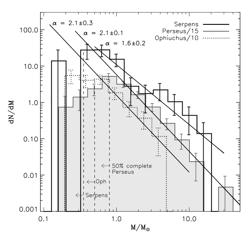
Differential () core mass distributions (CMDs) of 1.1 mm sources in Serpens, Perseus, and Ophiuchus are shown in Figure 16, with those of Perseus and Ophiuchus scaled down for clarity. Error bars reflect statistical uncertainties. Dashed lines indicate empirical 50% completeness limits for average sized sources in each cloud, which are determined as described in § 5.1 and in Paper I. Mass distributions include all 1.1 mm cores in each cloud, including those that may be associated with embedded protostellar sources.
The shape of the Ophiuchus and Perseus mass distributions are quite similar above their respective completeness limits ( in Ophiuchus and in Perseus). Fitting a power law () to the CMDs, we find that they both have a best fit slope of , although the error is larger on the slope for Ophiuchus () than for Perseus (). The slope of the Serpens CMD is marginally different (), being flatter than in the other two clouds by approximately .
The two-sided Kolmogorov-Smirnov test indicates a high probability (46%) that the Perseus and Ophiuchus mass distributions are representative of the same parent population. Conversely, the probabilities that the Serpens core masses are sampled from the same population as the Perseus (prob%) or Ophiuchus (prob%) masses are much lower. Although it is possible that the lower linear resolution in Perseus and Serpens has lead to larger masses via blending, the test we conducted to increase the effective beam size in the Ophiuchus map did not appreciably change the shape of the Ophiuchus mass distribution (see Figure 10).
If the shape of the CMD is a result of the fragmentation process, then the slope of the CMD can be compared to models, e.g. of turbulent fragmentation. Padoan & Nordlund (2002) argue that turbulent fragmentation naturally produces a power law with , consistent with the slopes we measure in Perseus and Ophiuchus (), but not with Serpens (). Recently Ballesteros-Paredes et al. (2006, hereafter BP06) have questioned that result, finding that the shape of the CMD depends strongly on the Mach number of the turbulence in their simulations. The BP06 smoothed particle hydrodynamics (SPH) simulations show that higher Mach numbers result in a larger number of sources with lower mass and a steep slope at the high mass end (their Figure 5). Conversely, lower Mach numbers favor sources with higher mass, resulting in a smaller number of low mass sources, more high mass cores, and a shallower slope at the high mass end.
Using an analytic argument, Padoan & Nordlund (2002) also note a relationship between core masses and Mach numbers, predicting that the mass of the largest core formed by turbulent fragmentation should be inversely proportional to the square of the Alfvénic Mach number on the largest turbulent scale . Given that our ability to accurately measure the maximum core mass is limited by resolution, small number statistics, and cloud distance differences, we focus here on the overall CMD shapes.
To compare our observational results to the simulations of BP06, we estimate the sonic Mach number in each cloud. Here is the observed rms velocity dispersion, is the isothermal sound speed, and is the mean molecular weight per particle. Large 13CO maps of Perseus and Ophiuchus observed with FCRAO at a resolution of 44″ are publicly available as part of “The COMPLETE Survey of Star Forming Regions”222http://cfa-www.harvard.edu/COMPLETE/ (COMPLETE; Goodman et al., 2004; Ridge et al., 2006). Average observed rms velocity dispersions kindly provided by the COMPLETE team are km s-1 in Perseus, km s-1 in Ophiuchus, and km s-1 in Serpens (J. Pineda, personal communication). These were measured by masking out all positions in the map that have peak temperatures with a S/N less than 10, fitting a Gaussian profile to each, and taking an average of the standard deviations.
We note that the value of km s-1 for Perseus is smaller than a previous measurement of km s-1 based on AT&T Bell Laboratory 7 m observations of a similar area of the cloud (Padoan et al., 2003). The smaller value derived by the COMPLETE team is most likely a consequence of the method used: a linewidth is calculated at every position and then an average of these values is taken. In contrast to calculating the width of the averaged spectrum this method removes the effects of velocity gradients across the cloud. The different resolutions of the surveys (44″ and 0.07 km s-1 for the COMPLETE observations, 100″ and 0.27 km s-1 for the Padoan et al. observations) may also play a role. Sources of uncertainty in the linewidth measurement are not insignificant, and include the possibility that 13CO is optically thick to an unknown degree, and the fact that line profiles are not necessarily well fit by a gaussian, especially in Perseus where the lines sometimes appear double-peaked.
Assuming that the sound speed is similar in all three clouds, the relative velocity dispersions suggest that turbulence is more important in Serpens than in Perseus or Ophiuchus, by factors of approximately 1.5 and 2, respectively. Mach numbers calculated using the observed and assuming a gas kinetic temperature of 10 K are (Serpens), (Perseus), and (Ophiuchus). We focus on Serpens and Ophiuchus, as they are the most different. Serpens is observed to have a higher Mach number than Ophiuchus, but the CMD indicates a larger number of high mass cores, a shallower slope at the high mass end, and a dearth of low mass cores compared to Ophiuchus. This result is contrary to the trends found by BP06, which would predict a steeper slope and more low mass cores in Serpens.333It should be noted that the shape of the CMDs presented by BP06 depend on the type of numerical code used, and not on the cloud Mach number alone. Here we have compared to the BP06 SPH simulations (their Figure 5); for the BP06 total variation diminishing (TVD) method (their Figure 4), a larger number of low mass cores are again seen for higher Mach numbers, but the CMD slopes at the high mass end are independent of Mach number.
One core of relatively high mass is measured in the degraded-resolution map of Ophiuchus, as is expected for blending at lower resolution (Figure 10), making the difference between the Serpens and Ophiuchus CMDs less dramatic. The degraded-resolution CMD for Ophiuchus still has a steeper slope () than the Serpens CMD, however, and a larger fraction of low mass sources: 81% of sources in the degraded-resolution Ophiuchus sample have compared to 49% in the Serpens sample.
More accurate measurements of the Mach number and higher resolution studies of the relative CMD shapes will be necessary to fully test the BP06 prediction, given that uncertainties are currently too large to draw firm conclusions. As both numerical simulations and observations improve, however, the observed CMD and measurements of the Mach number will provide a powerful constraint on turbulent star formation simulations.
Comparing the shape of the CMD to the stellar initial mass function (IMF) may give insight into what determines final stellar masses: the initial fragmentation into cores, competitive accretion, or feedback processes. The shape of the local IMF is still uncertain (Scalo, 2005), but recent work has found evidence for a slope of for stellar masses , somewhat steeper than the slopes we observe in all three clouds. For example, Reid et al. (2002) find above 0.6 M⊙, and above 1 M⊙. Chabrier (2003) suggests (), while Schröder & Pagel (2003) finds for M⊙ and for M⊙. For reference, the Salpeter IMF has a slope of (Salpeter, 1955).
For comparison to the IMF, we would ideally like to construct a CMD that includes starless cores only, so that it is a measure of the mass initially available to form a star. Although we cannot separate prestellar cores from more evolved objects with millimeter data alone, we are currently comparing the Bolocam maps with c2d Spitzer Legacy maps of the same regions, which will allow us to distinguish prestellar cores from those with internal luminosity sources (M. Enoch et al. 2007, in preparation).
5.6. Clustering
We use the two-point correlation function,
| (5) |
as a quantitative measure of the clustering of cores. Here is the number of core pairs with separation between and , and is similar but for a random distribution (see Paper I). Thus is a measure of excess clustering over a random distribution, as a function of separation.
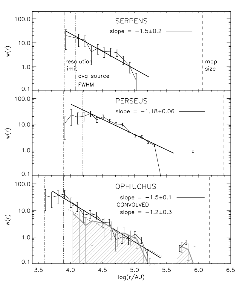
Figure 17 plots the cloud two-point correlation functions, with the best fit power laws, , shown. The average linear source FWHM size is indicated, as well as the minimum possible separation (the beam size), and the linear map size. The best fit slopes to for Serpens (), Perseus (), and Ophiuchus () are consistent within , but there is an indication both from the slopes and a visual examination of the plot that falls off more steeply in Serpens and Ophiuchus than in Perseus. A shallower slope suggests that clustering remains strong out to larger scales in Perseus than in the other two clouds.
We do find that a broken power law with slopes of (AU) and (AU) is a better fit to the Serpens correlation function than a single power law, indicating that clustering remains strong to intermediate scales, as in Perseus, but then drops off quickly. Also shown in Figure 17 is for the degraded-resolution Ophiuchus sample (gray hatched curve). The degraded-resolution sample is fit by a shallower slope () because there are fewer sources at small separations, but it is broadly consistent with the original Ophiuchus sample.
Our general conclusion that clustering of 1.1 mm sources remains strong over larger scales in Perseus than in Serpens and Ophiuchus can also be reached by visually examining each map. Perseus has highly clustered regions spread over a larger area as well as a number of more distributed sources, whereas Serpens and Ophiuchus have a single main cluster with fewer small groups spread throughout the cloud.
A few caveats should be noted here. First, the fact that clustering seems to extend over larger scales in Perseus could simply be due to the fact that Perseus has more widely separated regions of star formation, and the physical association of all these regions has not been firmly established. Second, the map of Serpens covers a much smaller linear area than that of Perseus (30 pc2 versus 140 pc2); we need to be sure that the steepening of the slope in Serpens is not caused by the map size. This was confirmed by taking a piece of the Perseus map equal in size to the Serpens map and recalculating . Although the value of the slope changed slightly, the smaller map size did not cause the slope to steepen at large separations. A more serious issue is that the overall amplitude, but not the slope, of depends on how large an area the random distribution covers. We choose each random distribution such that the largest pair separation is similar to the largest pair separation in the real data. For Serpens and Ophiuchus this means that the random distribution does not cover the entire observed area.
Finally, we look at two other measures of clustering: the peak number of cores per square parsec, and the median separation of cores. Although the median separation of cores is much smaller in Ophiuchus ( AU) than in Perseus ( AU) or Serpens ( AU), the median separation in the degraded-resolution Ophiuchus map ( AU) is consistent with the other two clouds. Imposing a uniform flux limit of across all three clouds, equivalent to the limit in the shallowest map (Perseus), does not significantly change these results.
We calculate the number of cores within one square parsec at each point in the map, and take the peak value to be the peak number of cores per square parsec. The peak values are in Serpens, in Perseus, and in the original Ophiuchus map. Differences in linear resolution and completeness both have an effect in this case; the peak number in Ophiuchus falls to 20 pc-2 when using a uniform flux limit, and to 12 pc-2 in the degraded-resolution map. The peak number of cores per parsec provides further evidence that clustering is stronger in Perseus than in the other two clouds.
5.7. Relationship to Cloud Column Density
In contrast to the extinction map, which is a measure of the general cloud (line-of-sight averaged) column density, the 1.1 mm map is sensitive only to regions of high volume density (see § 5.1). A comparison of the two tells us, therefore, about the relationship between dense star-forming structures and the column density of the larger-scale cloud. A visual comparison of the 1.1 mm maps of each cloud with visual extinction maps derived from the reddening of background stars (e.g. Figure 5) suggests that 1.1 mm cores are generally found in regions of the cloud with high .
Figure 18 quantifies the relationship between dense cores and the surrounding cloud column density by plotting the cumulative fraction of 1.1 mm cores in each cloud as a function of cloud . In all three clouds the majority of cores are found at high cloud column density (). The levels above which 75% of cores are found in each cloud are indicated by thin lines in Figure 18: 75% of 1.1 mm cores in Perseus, Serpens, and Ophiuchus are found at visual extinctions of , , and , respectively. Although there is not, in general, a strict extinction threshold for finding cores, below these levels the likelihood of finding a 1.1 mm core is very low. Only in Ophiuchus does there appear to be a true threshold; only two cores are found at in this cloud.
The cumulative distribution for the degraded resolution Ophiuchus sample is nearly identical to the original Ophiuchus sample, but shifted to lower by 1–2 mag. For the degraded resolution map, 75% of cores are found at . Based on this result and the value for the original Ophiuchus sample, we adopt for the 75% level in Ophiuchus. Requiring that all cores in the Perseus and Serpens sample meet the detection threshold for Ophiuchus (approximately 110 mJy) changes the distributions negligably. Only for Serpens is the 75% level increased slightly, from to .
Cloud to cloud differences could indicate variations in the core formation process with environment, differing degrees of sub-structure in the clouds, or varying amounts of foreground extinction. Note that in Papers I and II we found extinction “thresholds” for Perseus and Ophiuchus, using a different analysis that looked at the probability of finding a 1.1 mm core as a function of , of and , respectively. Those values were derived using 2MASS-only maps, rather than the c2d extinction maps used here.
Johnstone et al. (2004) have suggested an extinction threshold for forming dense cores in Ophiuchus at , based on the lowest at which SCUBA cores were observed to have sizes and fluxes consistent with those of stable Bonnor-Ebert spheres. We find that most Bolocam cores in Ophiuchus are found at even higher extinctions (75% at ); the discrepancy likely arises from differences in the extinction maps used. Johnstone et al. (2004) used a 2MASS-derived extinction map, while the c2d extinction map used here includes IRAC data as well and probes somewhat higher values. Hatchell et al. (2005) find no evidence for an extinction threshold in Perseus using SCUBA data, but Kirk, Johnstone & Di Francesco (2006), also using SCUBA data, find a threshold of . Despite differences in detail, the relative 75% levels found here (highest in Ophiuchus and lowest in Perseus) are consistent with the relative values of previous extinction threshold measurements in Perseus and Ophiuchus.
An extinction threshold has been predicted by McKee (1989) for photoionization-regulated star formation in magnetically supported clouds. In this model star formation is governed by ambipolar diffusion, which depends on ionization levels in the cloud. Core collapse and star formation will occur only in shielded regions of a molecular cloud where . Johnstone et al. (2004) note that it is not clear how turbulent models of star formation would produce an extinction threshold for star-forming objects, and interpret such a threshold as evidence for magnetic support.
5.8. Efficiency of Forming Cores
Another interesting measure of global cloud conditions is the fraction of cloud mass contained in dense cores. Table 3 lists the cloud area and cloud mass within increasing contours, calculated from the c2d visual extinction maps, as well as the total mass in cores within the same extinction contour. Cloud masses are calculated from the c2d maps (§ 3.1.3, Eq. 2). The total cloud mass within is 3470 M⊙for Serpens, 7340 M⊙for Perseus, and 3570 M⊙for Ophiuchus.
Within a given contour, the mass ratio is defined as the ratio of total core mass to total cloud mass, and is a measure of the efficiency of core formation at that level. For example, the mass ratio at the contour is equivalent to the fraction of total cloud mass that is contained in dense cores. In each cloud 1.1 mm cores account for less than 5% of the total cloud mass. The mass ratios at are similar in all three clouds: 3.8% in Perseus, 2.7% in Serpens, and 1.2% in Ophiuchus. If we restrict ourselves to in each cloud, which is reasonable given that the Serpens map was only designed to cover , the mass ratio is still low in all three clouds (%), and remains higher in Perseus (7%) than in Serpens (4%) or Ophiuchus (2%). Low mass ratios are consistent with measurements of the overall star-formation efficiency of , which suggests that molecular cloud material is relatively sterile (e.g. Evans, 1999; Leisawitz et al., 1989).
Johnstone et al. (2004) find a mass ratio of 2.5% in a survey of approximately deg2 of Ophiuchus, quite similar to our result. Note, however, that the Johnstone et al. (2004) core masses (and mass ratio) should be multiplied by a factor of 1.5 to compare to our values, due to differences in assumed values of , , and . In a similar analysis of 3.5 deg2 in Perseus, also using SCUBA data, Kirk, Johnstone & Di Francesco (2006) found a mass ratio for of only 1%. The difference between this result and our value arises primarily from the smaller core masses of those authors, which should be multiplied by 2.5 to compare to ours.
In all three clouds the mass ratio rises with increasing contour, indicating that in high extinction regions a greater percentage of cloud mass has been assembled into cores, consistent with the idea that star formation is more efficient in dense regions. Although this is an intuitively obvious result, it is not a necessary one. If, for example, a constant percentage of cloud mass were contained in dense cores at all column densities, there would be a large number of dense cores lying in a low background. On the other hand, a molecular cloud might consist of large regions of uniformly high extinction in which we would find no 1.1 mm cores because there is no sub-structure, and millimeter cores require high density contrast (see § 5.1).
At higher levels, mass ratios vary considerably from cloud to cloud. The mass ratio remains fairly low in Ophiuchus, with a maximum value of 9% at . In contrast, the mass ratio rises rapidly in Serpens to 65% at , which may suggest that Serpens has formed cores more efficiently than Ophiuchus at high .
6. Summary
This work completes a three-cloud study of the millimeter continuum emission in Perseus, Ophiuchus, and Serpens. We examine similarities and differences in the current star formation activity within the clouds using large-scale 1.1 mm continuum maps completed with Bolocam at the CSO. In total, our surveys cover nearly 20 deg2 with a resolution of 31″ (7.5 deg2 in Perseus, 10.8 deg2 in Ophiuchus, and 1.5 deg2 in Serpens), and we have assembled a sample of 200 cores (122 in Perseus, 44 in Ophiuchus, and 35 in Serpens). Point mass detection limits vary from approximately 0.1 to 0.2 M⊙ depending on the cloud. The results presented here provide an unprecedented global picture of star formation in three clouds spanning a range of diverse environments.
These Bolocam 1.1 mm observations naturally select dense cores with cm-3 and density contrast compared to the background cloud of at least . We test instrumental biases and the effects of cloud distance by degrading the resolution of the Ophiuchus map to match the distance of Perseus and Serpens. We find that linear resolution strongly biases measured linear deconvolved source sizes and mean densities, but not the mass distribution slope. Angular deconvolved sizes are less strongly affected by cloud distance.
Rather than a true physical difference, the small mean linear deconvolved sizes in Ophiuchus ( AU) compared to Perseus ( AU) and Serpens ( AU) are likely a result of observing sources with power law density profiles, which do not have a well defined size, at a distance of 125 pc in Ophiuchus versus 250 pc in Perseus and 260 pc in Serpens. The observed mean angular deconvolved sizes and axis ratios in each cloud suggest average power law indices ranging from to 1.7 (Y03).
Sources in Perseus exhibit the largest range in sizes, axis ratios, and densities, whereas sources in both Serpens and Ophiuchus display a fairly narrow range of sizes for a large range of masses. We suggest that this is indicative of a greater variety of physical conditions in Perseus, supported by the fact that Perseus contains both dense clusters of millimeter sources and more isolated distributed objects. A wide range in angular deconvolved sizes may also imply a range in the power law index of source profiles in Perseus (Y03).
The slope of the clump mass distribution for both Perseus and Ophiuchus is , marginally different than the Serpens slope of . Only Perseus and Ophiuchus are consistent within the substantial errors with the stellar initial mass function () and with the slope predicted for turbulent fragmentation () by Padoan & Nordlund (2002).
Turbulent fragmentation simulations by BP06 predict that higher cloud Mach numbers should result in a large number of low mass cores, and low Mach numbers in a smaller number of higher mass cores. Given the measured Mach numbers of in Serpens, 3.6 in Perseus and 2.3 in Ophiuchus, our observed core mass distribution (CMD) shapes are inconsistent with the turbulent fragmentation prediction from BP06. We cannot rule out a turbulent fragmentation scenario, however, due to uncertainties in the observations and in our assumptions.
We argue that clustering of 1.1 mm sources remains stronger out to larger scales in Perseus, based on the slope of the two-point correlation function (-1.5 in Serpens and Ophiuchus, and -1.2 in Perseus). This result is supported by the fact that the peak number of cores per square parsec is larger in Perseus () than in Serpens () or the degraded-resolution Ophiuchus map ().
Finally, we examine relationship between dense cores and the local cloud column density, as measured by visual extinction (). Extinction thresholds for star formation have been suggested based on both theory and observation (McKee, 1989; Johnstone et al., 2004). Although in general we do not observe a strict threshold, dense 1.1 mm cores do tend to be found at high : 75% of cores in Perseus are found at , in Serpens at , and in Ophiuchus at . Our results confirm that forming dense cores in molecular clouds is a very inefficient process, with 1.1 mm cores accounting for less than 10% of the total cloud mass in each cloud. This result is consistent with measurements of low star formation efficiencies of a few percent from studies of the stellar content of molecular clouds (e.g. Evans, 1999).
While millimeter-wavelength observations can provide a wealth of information about the detailed properties of star forming cores as well as insight into the large scale physical properties of molecular clouds, they do not tell a complete story. Detecting and understanding the youngest embedded protostars currently forming within those cores requires information at mid- to far-infrared wavelengths. The Bolocam maps for all three clouds presented here are coordinated to cover the same regions as the c2d Spitzer Legacy IRAC and MIPS maps of Serpens, Perseus, and Ophiuchus. Combining millimeter and Spitzer data for these clouds will allow us to separate starless cores from cores with embedded luminosity sources and to better understand the evolution of cores through the early Class 0 and Class I protostellar phases. Synthesis and analysis of the combined data set is currently underway (M. Enoch et al. 2007, in preparation).
References
- Ballesteros-Paredes et al. (2006) Ballesteros-Paredes, J., Gazol, A., Kim, J., Klessen, R. S., Jappsen, A-K., & Tejero, E., 2006, ApJ, 637, 384
- Bohlin et al. (1978) Bohlin, R. C., Savage, B. D., & Drake, J. F. 1978, ApJ, 224, 132
- Cambrésy (1999) Cambrésy, L. 1999, A&A, 345, 965
- Casali, Eiroa, & Duncan (1993) Casali, M. M., Eiroa, C., Duncan, W. D. 1993, A&A, 275, 195
- Chabrier (2003) Chabrier, G. 2003, PASP, 115, 763
- Davis et al. (1999) Davis, C. J., Matthews, H. E., Ray, T. P., Dent, W. R. F., & Richer, J. S. 1999, MNRAS, 309, 141
- Di Francesco et al. (2005) Di Francesco, J., Evans, N.J. II, Caselli, P., Myers, P.C., Shirley, Y., Aikawa, Y., & Tafalla, M., ”An Observational Perspective of Low-Mass Dense Cores I: Internal Physical and Chemical Properties,” Protostars and Planets V, 2005
- Djupvik et al. (2006) Djupvik, A. A., André, Ph., Bontemps, S., Motte, F., Olofsson, G., Gålfalk, M., & Florén, H.-G. 2006, A&A, 485, 789
- Eiroa & Casali (1992) Eiroa, C. & Casali, M. M.. 1992, A&A, 262, 468
- Enoch et al. (2006) Enoch, M. L., et al. 2006, ApJ, 638, 293
- Evans (1999) Evans, N. J. 1999, ARA&A, 37, 311
- Evans et al. (2001) Evans, N. J., II, Rawlings, J. M. C., Shirley, Y. L., & Mundy, L. G. 2001, ApJ, 557, 193
- Evans et al. (2003) Evans, N. J., II, et al. 2003, PASP, 115, 965
- Evans et al. (2006) Evans, N. J., II, et al. 2006, Final Delivery of Data from the c2d Legacy Project: IRAC and MIPS (Pasadena: Caltech), http://data.spitzer.caltech.edu
- Glenn et al. (2003) Glenn, J., et al. 2003, Proc. SPIE, 4855, 30
- Goodman et al. (2004) Goodman, A. A., & the COMPLETE Team, 2004, in Star Formation in the Interstellar Medium (San Francisco: ASP)
- Harvey et al. (2006) Harvey, P. M., et al. 2006, ApJ, 644, 307
- Harvey et al. (2007) Harvey, P. M., et al. 2007, ApJ, in press
- Hatchell et al. (2005) Hatchell, J., Richer, J. S., Fuller, G. A., Qualtrough, C. J., Ladd, E. F., & Chandler, C. J. 2005, A&A, 440, 151
- Huard et al. (2006) Huard, T. L., et al. 2006, ApJ, 640, 391
- Hurt & Barsony (1996) Hurt, R. L., Barsony, M. 1996, ApJ, 460, L45
- Johnstone et al. (2000) Johnstone, D., Wilson, C. D., Moriarty-Schieven, G., Joncas, G., Smith, G., Gregersen, E., & Fich, M. 2000, ApJ, 545, 327
- Johnstone et al. (2004) Johnstone, D., DiFrancesco, J., & Kirk, H. 2004, ApJ, 45, 611L
- Jørgensen et al. (2006) Jørgensen, J., et al. 2006, ApJ, submitted
- Kirk et al. (2005) Kirk, J. M., Ward-Thompson, D., & André, P. 2005, MNRAS, 360, 1506
- Kirk, Johnstone & Di Francesco (2006) Kirk, H., Johnstone, D., & Di Francesco, J. 2006, ApJ, 646, 1009
- Larson (1981) Larson, R. B., 1981, MNRAS, 194, 809
- Lada et al. (1999) Lada, C. J., Alves, J., & Lada, E. A. 1999, in The Physics and Chemistry of the Interstellar Medium, eds. V. Ossenkopf, J. Stutzki, G. Winnewisser, 161
- Laurent et al. (2005) Laurent, G., et al. 2005, ApJ, 623, 742
- Larsson et al. (2000) Larsson, B., et al. 2000 A&A, 363, 253
- Leisawitz et al. (1989) Leisawitz, D., Bash, F., & Thaddeus, P. 1989, ApJS, 70, 731
- Mac Low & Klessen (2004) Mac Low, M.-M. & Klessen, R. S. 2004, Reviews of Modern Physics, 76, 125
- McKee (1989) McKee, C. F. 1989, ApJ, 345, 782
- Myers (1998) Myers, P. C. 1998, ApJ, 496, L109
- Ossenkopf & Henning (1994) Ossenkopf, V., & Henning, Th. 1994, A&A, 291, 943
- Padoan & Nordlund (2002) Padoan, P., & Nordlund, Å. 2002, ApJ, 576, 870
- Padoan et al. (2003) Padoan, P., Goodman, A. A., & Juvela, M. 2003, ApJ, 588 881
- Reid et al. (2002) Reid, I. N., Gizis, J. E., & Hawley, S. L. 2002, AJ, 124, 2721
- Ridge et al. (2006) Ridge, N. A., et al. 2006, AJ, 131, 2921
- Salpeter (1955) Salpeter, E. E. 1955, ApJ, 121, 161
- Scalo (2005) Scalo, J., 2005 in The Stellar Initial Mass Function Fifty Years Later, Kluwer Academic Publishers, ed. E. Corbelli, F. Palla, and H. Zinnecker, p. 23
- Schröder & Pagel (2003) Schröder, K.-P., & Pagel, B. E. J. 2003, MNRAS, 343, 1231
- Shirley et al. (2002) Shirley, Y. L., Evans, N. J., II, & Rawlings, J. M. C. 2002, ApJ, 575, 337
- Shu et al. (1978) Shu, F. H., Adams, F. C., & Lizano, S. 1978, ARA&A, 25, 23
- Stanke et al. (2006) Stanke, T., Smith, M. D., Gredel, R., Khanzadyan, T. 2006, A&A, 447, 609
- Straizys et al. (1996) Straizys, V., Cernis, K., & Bartasiute, S. 1996, Baltic Astronomy, 5, 125
- Testi & Sargent (1998) Testi, L. & Sargent, A. I. 1998, ApJ, 508, L91
- Weingartner & Draine (2001) Weingartner, J. C. & Draine, B. T. 2001, ApJ, 548, 296
- Williams et al. (1994) Williams, J. P., deGeus, E. J., & Blitz, L. 1994, ApJ, 428, 693
- Young et al. (2003) Young, C. H., Shirley, Y. L., Evans, N. J., II, & Rawlings, J. M. C. 2003, ApJS, 145, 111
- Young et al. (2006) Young, K. E., et al. 2006, ApJ, 644, 326
| ID | RA (2000) | Dec (2000) | Peak | S/N | other names | MIPS source? |
|---|---|---|---|---|---|---|
| () | () | (mJy/beam) | ||||
| Bolo1 | 18 28 23.1 | +00 26 34.6 | 95 (12) | 5.0 | N | |
| Bolo2 | 18 28 44.0 | +00 53 02.8 | 198 (12) | 9.9 | N | |
| Bolo3 | 18 28 45.8 | +00 51 32.4 | 227 (12) | 13.7 | IRAS 18262+0050 | Y |
| Bolo4 | 18 28 47.2 | +00 50 45.1 | 145 (10) | 7.1 | N | |
| Bolo5 | 18 28 48.3 | +00 14 51.5 | 73 (9) | 5.8 | N | |
| Bolo6 | 18 28 50.8 | +00 50 28.6 | 115 (10) | 7.3 | N | |
| Bolo7 | 18 28 53.0 | +00 19 03.6 | 119 (11) | 5.4 | Y | |
| Bolo8 | 18 28 55.2 | +00 29 28.0 | 617 (13) | 30.8 | IRAS 18263+0027; MMS1 (2) | Y |
| Bolo9 | 18 28 55.9 | +00 48 30.3 | 141 (10) | 9.1 | N | |
| Bolo10 | 18 28 56.6 | +00 19 10.4 | 107 (11) | 5.7 | N | |
| Bolo11 | 18 28 57.3 | +00 48 06.5 | 162 (11) | 10.9 | N | |
| Bolo12 | 18 28 58.4 | +00 47 35.7 | 172 (11) | 12.0 | N | |
| Bolo13 | 18 29 00.2 | +00 30 19.8 | 239 (15) | 5.5 | Y | |
| Bolo14 | 18 29 07.0 | +00 30 41.5 | 1016 (14) | 59.2 | IRAS 18265+0028; MMS2 (2) | Y |
| Bolo15 | 18 29 09.6 | +00 31 36.9 | 626 (14) | 33.0 | MMS3 (2) | Y |
| Bolo16 | 18 29 13.5 | +00 32 12.6 | 175 (13) | 5.8 | N | |
| Bolo17 | 18 29 16.4 | +00 18 15.4 | 82 (8) | 6.7 | IRAS 18267+0016 | Y |
| Bolo18 | 18 29 19.3 | +00 33 29.1 | 104 (12) | 6.0 | N | |
| Bolo19 | 18 29 31.5 | +00 26 49.3 | 279 (14) | 14.8 | MMS4 (2) | N |
| Bolo20 | 18 29 31.9 | +01 19 00.9 | 337 (13) | 18.3 | Y | |
| Bolo21 | 18 29 43.4 | +00 36 25.2 | 129 (11) | 7.7 | N | |
| Bolo22 | 18 29 48.8 | +01 16 50.6 | 1694 (16) | 80.7 | SMM 9 (1); S68N | Y |
| Bolo23 | 18 29 50.2 | +01 15 24.6 | 3010 (20) | 138 | SMM 1 (1); FIRS 1 | Y |
| Bolo24 | 18 29 53.8 | +00 36 10.1 | 202 (10) | 17.2 | IRAS 18273+0034 | Y |
| Bolo25 | 18 29 57.4 | +01 13 14.9 | 1980 (23) | 62.7 | SMM 4 (1) | Y |
| Bolo26 | 18 29 59.2 | +01 14 07.4 | 1331 (19) | 43.0 | SMM 3 (1) | Y |
| Bolo27 | 18 30 00.3 | +01 10 37.8 | 425 (19) | 14.5 | Y | |
| Bolo28 | 18 30 00.7 | +01 12 56.5 | 1266 (19) | 34.3 | SMM 2 (1) | Y |
| Bolo29 | 18 30 01.0 | +01 11 49.1 | 979 (19) | 33.5 | SMM 11 (1) | Y |
| Bolo30 | 18 30 02.5 | +01 15 24.5 | 319 (16) | 11.3 | SMM 8 (1) | Y |
| Bolo31 | 18 30 02.8 | +01 08 38.3 | 214 (16) | 10.0 | Y | |
| Bolo32 | 18 30 05.7 | +00 39 32.2 | 105 (12) | 5.0 | Y | |
| Bolo33 | 18 30 06.4 | +00 42 37.0 | 126 (11) | 8.3 | Y | |
| Bolo34 | 18 30 08.2 | +01 13 11.5 | 153 (11) | 7.8 | N | |
| Bolo35 | 18 30 14.7 | +01 13 52.6 | 85 (11) | 5.6 | N |
Note. — Numbers in parentheses are errors. The peak flux density is the peak value per beam in the pixel-1 unfiltered map (without the optimal filter applied). The uncertainty in the peak flux density is the local rms beam-1 and does not include an additional 15% systematic uncertainty from calibration uncertainties and residual errors after iterative mapping. Other names listed are the most common identifications from the literature, and are not meant to be a complete list. A 1.1 mm source is considered coincident with a MIPS source if the position is within of a source from the c2d catalog (Harvey et al., 2007). References – (1) Casali, Eiroa, & Duncan (1993); (2) Djupvik et al. (2006)
| ID | Flux() | Flux() | Flux() | Total Flux | Mass (10K) | Peak | FWHM | FWHM | PA | Morphology11The morphology keywords given indicates whether the source is multiple (within of another source), extended (major axis FW at ), elongated (axis ratio at ), round (axis ratio at ), or weak (peak flux density less than 5 times the rms pixel-1 in the unfiltered map). | |
|---|---|---|---|---|---|---|---|---|---|---|---|
| (Jy) | (Jy) | (Jy) | (Jy) | () | (mag) | (minor,) | (major,) | () | cm-3 | ||
| Bolo1 | 0.137 (0.016) | 0.25 (0.03) | 0.65 (0.07) | 8 | 52 (1.0) | 62 (1.2) | 55 (8) | 1.0 | extended,elongated,weak | ||
| Bolo2 | 0.282 (0.017) | 0.51 (0.03) | 1.34 (0.08) | 17 | 51 (0.5) | 63 (0.6) | -57 (4) | 2.1 | multiple,extended,elongated | ||
| Bolo3 | 0.324 (0.015) | 0.382 (0.019) | 1.00 (0.05) | 19 | 43 (0.4) | 55 (0.5) | -77 (3) | 3.2 | multiple,extended,round | ||
| Bolo4 | 0.226 (0.013) | 0.28 (0.017) | 0.73 (0.04) | 12 | 43 (0.5) | 55 (0.6) | 49 (4) | 2.2 | multiple,extended,elongated | ||
| Bolo5 | 0.094 (0.013) | 0.16 (0.02) | 0.41 (0.06) | 6 | 50 (1.2) | 63 (1.4) | -68 (8) | 7 | extended,round,weak | ||
| Bolo6 | 0.172 (0.013) | 0.210 (0.016) | 0.55 (0.04) | 10 | 46 (0.6) | 62 (0.8) | -40 (3) | 1.1 | multiple,extended,elongated | ||
| Bolo7 | 0.162 (0.015) | 0.162 (0.015) | 0.42 (0.04) | 10 | 46 (0.8) | 57 (0.9) | -30 (7) | 1.0 | multiple,extended,elongated | ||
| Bolo8 | 0.933 (0.018) | 1.99 (0.04) | 2.63 (0.04) | 6.87 (0.12) | 52 | 62 (0.2) | 74 (0.2) | 68 (1) | 5.2 | multiple,extended,round | |
| Bolo9 | 0.169 (0.010) | 0.44 (0.03) | 12 | 38 (0.5) | 61 (0.7) | -58 (2) | 1.5 | multiple,extended,elongated | |||
| Bolo10 | 0.146 (0.015) | 0.146 (0.015) | 0.38 (0.04) | 9 | 51 (0.8) | 54 (0.9) | 11 (25) | 8 | multiple,extended,elongated | ||
| Bolo11 | 0.199 (0.011) | 0.52 (0.03) | 14 | 37 (0.4) | 61 (0.7) | -59 (2) | 1.8 | multiple,round, | |||
| Bolo12 | 0.246 (0.014) | 0.246 (0.014) | 0.64 (0.04) | 15 | 39 (0.4) | 58 (0.6) | -65 (2) | 2.2 | multiple,extended,elongated | ||
| Bolo13 | 0.36 (0.02) | 0.36 (0.02) | 0.94 (0.05) | 20 | 52 (0.5) | 59 (0.5) | -78 (6) | 1.7 | multiple,extended,round | ||
| Bolo14 | 1.381 (0.019) | 2.16 (0.03) | 5.65 (0.09) | 86 | 47 (0.1) | 54 (0.1) | -44 (2) | 1.5 | multiple,extended,elongated | ||
| Bolo15 | 0.856 (0.018) | 0.856 (0.018) | 2.24 (0.05) | 53 | 44 (0.2) | 56 (0.2) | -27 (1) | 6.5 | multiple,extended,round | ||
| Bolo16 | 0.222 (0.018) | 0.27 (0.02) | 0.71 (0.06) | 15 | 42 (0.5) | 62 (0.8) | 32 (3) | 1.8 | multiple,extended,elongated | ||
| Bolo17 | 0.118 (0.011) | 0.24 (0.02) | 0.4 (0.03) | 0.40 (0.03) | 1.05 (0.09) | 7 | 80 (1.1) | 97 (1.3) | -66 (5) | 3 | extended,elongated |
| Bolo18 | 0.144 (0.016) | 0.25 (0.03) | 0.65 (0.08) | 9 | 48 (0.8) | 71 (1.2) | -41 (3) | 9 | multiple,extended,elongated,weak | ||
| Bolo19 | 0.41 (0.018) | 0.85 (0.04) | 1.28 (0.06) | 1.28 (0.06) | 3.34 (0.14) | 24 | 74 (0.5) | 89 (0.6) | -74 (3) | 1.3 | extended,elongated |
| Bolo20 | 0.494 (0.018) | 1.01 (0.04) | 1.57 (0.05) | 1.57 (0.05) | 4.11 (0.14) | 29 | 87 (0.5) | 90 (0.5) | 9 (11) | 1.2 | extended,elongated |
| Bolo21 | 0.177 (0.014) | 0.38 (0.03) | 0.38 (0.03) | 0.98 (0.07) | 11 | 53 (0.7) | 64 (0.8) | 47 (6) | 1.3 | multiple,extended,elongated | |
| Bolo22 | 2.32 (0.02) | 3.78 (0.04) | 9.86 (0.10) | 144 | 47 (0.1) | 57 (0.1) | 73 (1) | 2.3 | multiple,extended,round | ||
| Bolo23 | 3.8 (0.03) | 5.91 (0.05) | 5.91 (0.05) | 15.44 (0.14) | 256 | 46 (0.1) | 47 (0.1) | 39 (4) | 6.1 | multiple,extended,round | |
| Bolo24 | 0.291 (0.014) | 0.40 (0.02) | 1.04 (0.05) | 17 | 46 (0.4) | 55 (0.5) | -12 (4) | 2.9 | multiple,extended,elongated | ||
| Bolo25 | 2.75 (0.03) | 3.19 (0.04) | 8.33 (0.10) | 168 | 44 (0.1) | 51 (0.1) | 79 (1) | 2.9 | multiple,extended,round | ||
| Bolo26 | 1.9 (0.03) | 1.90 (0.03) | 4.95 (0.07) | 113 | 48 (0.1) | 59 (0.1) | -21 (1) | 1.0 | multiple,extended,round | ||
| Bolo27 | 0.65 (0.03) | 1.18 (0.05) | 3.09 (0.12) | 36 | 47 (0.3) | 69 (0.4) | 89 (1) | 4.6 | multiple,extended,elongated | ||
| Bolo28 | 1.9 (0.03) | 1.90 (0.03) | 4.96 (0.06) | 108 | 48 (0.1) | 59 (0.1) | -47 (1) | 1.0 | multiple,extended,round | ||
| Bolo29 | 1.41 (0.03) | 2.44 (0.05) | 6.37 (0.12) | 83 | 47 (0.1) | 59 (0.2) | -86 (1) | 1.4 | multiple,extended,round | ||
| Bolo30 | 0.43 (0.02) | 0.43 (0.02) | 1.13 (0.06) | 27 | 48 (0.4) | 55 (0.5) | 33 (5) | 2.6 | multiple,extended,elongated | ||
| Bolo31 | 0.32 (0.02) | 0.65 (0.04) | 0.65 (0.04) | 1.70 (0.11) | 18 | 45 (0.5) | 74 (0.8) | -65 (2) | 2.4 | multiple,extended,elongated | |
| Bolo32 | 0.151 (0.016) | 0.34 (0.03) | 0.34 (0.03) | 0.88 (0.08) | 9 | 57 (0.9) | 74 (1.2) | 50 (5) | 8 | extended,elongated | |
| Bolo33 | 0.12 (0.015) | 0.128 (0.019) | 0.34 (0.05) | 11 | 35 (0.9) | 39 (1.1) | 25 (17) | 6.9 | round | ||
| Bolo34 | 0.181 (0.015) | 0.216 (0.019) | 0.56 (0.05) | 13 | 40 (0.6) | 60 (0.9) | -70 (3) | 1.7 | multiple,extended,elongated | ||
| Bolo35 | 0.06 (0.011) | 0.16 (0.03) | 7 | 24 (1.1) | 61 (2.9) | -69 (4) | 2.4 | multiple,weak |
Note. — Masses are calculated according to Eq. 1 from the total flux density assuming a single dust temperature of K and a dust opacity at 1.1mm of cm2g-1. Peak is calculated from the peak flux density as in Eq. 3. FWHM and PAs are from an elliptical gaussian fit; the PA of the major axis is measured in degrees east of north. is the mean particle density as calculated from the total mass and the deconvolved average FWHM size. Numbers in parentheses are uncertainties. Uncertainties for masses are from photometry only, and do not include uncertainties from , , or , which can be up to a factor of a few or more. Uncertainties for the FWHM and PA are formal fitting errors from the elliptical gaussian fit; additional uncertainties of % apply to the FWHM, and to the PA (determined from simulations).
| Min. | Area | Cloud Mass | Percent | Core Mass | Percent | Mass Ratio11The Mass Ratio is computed from the ratio of total core mass to cloud mass within the same contour of . |
|---|---|---|---|---|---|---|
| mag | (%) | (M⊙) | (%) | (M⊙) | (%) | (%) |
| Serpens | ||||||
| 2 | 100 | 3470 | 100 | 92 | 100 | 2.7 |
| 4 | 97 | 3420 | 99 | 92 | 100 | 2.7 |
| 6 | 60 | 2560 | 74 | 92 | 100 | 3.6 |
| 8 | 28 | 1530 | 44 | 91 | 98 | 5.9 |
| 10 | 15 | 1010 | 29 | 91 | 98 | 9.0 |
| 12 | 9.4 | 740 | 21 | 89 | 96 | 12 |
| 14 | 6.0 | 540 | 15 | 89 | 96 | 16 |
| 16 | 3.9 | 390 | 11 | 86 | 93 | 22 |
| 18 | 2.6 | 290 | 8.3 | 83 | 90 | 29 |
| 20 | 2.0 | 230 | 6.7 | 79 | 85 | 34 |
| 25 | 1.0 | 130 | 3.7 | 61 | 66 | 47 |
| 30 | 0.4 | 60 | 1.7 | 39 | 42 | 65 |
| Perseus | ||||||
| 2 | 100 | 7340 | 100 | 278 | 97 | 3.8 |
| 4 | 55 | 5460 | 74 | 273 | 96 | 5.0 |
| 6 | 27 | 3620 | 49 | 258 | 91 | 7.1 |
| 8 | 14 | 2370 | 32 | 244 | 86 | 10 |
| 10 | 8.0 | 1620 | 22 | 205 | 72 | 13 |
| 12 | 4.8 | 1140 | 15 | 161 | 57 | 14 |
| 14 | 3.2 | 840 | 12 | 127 | 45 | 15 |
| 16 | 2.0 | 610 | 8.3 | 112 | 39 | 18 |
| 18 | 1.3 | 440 | 6.0 | 96 | 34 | 22 |
| 20 | 0.9 | 340 | 4.6 | 88 | 31 | 26 |
| 25 | 0.4 | 180 | 2.5 | 53 | 19 | 29 |
| 30 | 0.2 | 100 | 1.4 | 6.1 | 2.2 | 6.1 |
| Ophiuchus | ||||||
| 2 | 100 | 3570 | 100 | 44 | 100 | 1.2 |
| 4 | 55 | 2710 | 76 | 44 | 100 | 1.6 |
| 6 | 25 | 1830 | 51 | 40 | 92 | 2.2 |
| 8 | 14 | 1330 | 37 | 40 | 92 | 3.0 |
| 10 | 9.0 | 1070 | 30 | 40 | 92 | 3.7 |
| 12 | 7.0 | 940 | 26 | 40 | 92 | 4.3 |
| 14 | 5.6 | 820 | 23 | 40 | 92 | 4.9 |
| 16 | 4.6 | 730 | 20 | 40 | 92 | 5.5 |
| 18 | 3.8 | 640 | 18 | 39 | 90 | 6.1 |
| 20 | 3.1 | 560 | 16 | 37 | 84 | 6.6 |
| 25 | 2.0 | 400 | 11 | 32 | 73 | 8.0 |
| 30 | 1.2 | 260 | 7.3 | 23 | 52 | 8.8 |