Determination of the Far-Infrared Cosmic Background Using COBE/DIRBE and WHAM Data

Abstract

Determination of the cosmic infrared background (CIB) at far infrared wavelengths using COBE/DIRBE data is limited by the accuracy to which foreground interplanetary and Galactic dust emission can be modeled and subtracted. Previous determinations of the far infrared CIB (e.g., Hauser et al. 1998) were based on the detection of residual isotropic emission in skymaps from which the emission from interplanetary dust and the neutral interstellar medium were removed. In this paper we use the Wisconsin H$\alpha$ Mapper (WHAM) Northern Sky Survey as a tracer of the ionized medium to examine the effect of this foreground component on determination of the CIB. We decompose the DIRBE far infrared data for five high Galactic latitude regions into H I– and H$\alpha$–correlated components and a residual component. Based on FUSE H₂ absorption line observations, the contribution of an H₂–correlated component is expected to be negligible. We find the H$\alpha$–correlated component to be consistent with zero for each region, and we find that addition of an H$\alpha$– correlated component in modeling the foreground emission has negligible effect on derived CIB results. Our CIB detections and 2$\sigma$ upper limits are essentially the same as those derived by Hauser et al. and are given by $\nu I_{\nu}($nW m^-2 sr^-1) $<$ 75, $<$ 32, 25$\pm$8, and 13$\pm$3 at $\lambda$ = 60, 100, 140, and 240 $\mu$m, respectively. Our residuals have not been subjected to a detailed anisotropy test, so our CIB results do not supersede those of Hauser et al. We derive upper limits on the 100 $\mu$m emissivity of the ionized medium that are typically about 40% of the 100 $\mu$m emissivity of the neutral atomic medium. This low value may be caused in part by a lower dust-to-gas mass ratio in the ionized medium than in the neutral medium, and in part by a shortcoming of using H$\alpha$ intensity as a tracer of far infrared emission. If H$\alpha$ is not a reliable tracer, our analysis would underestimate the emissivity of the ionized medium, and both our analysis and the Hauser et al. analysis may slightly overestimate the CIB. We estimate the possible effect for the CIB to be only about 5%, which is much smaller than the quoted uncertainties. From a comparison of the Hauser et al. CIB results with the integrated galaxy brightness from Spitzer source counts, we obtain 2$\sigma$ upper limits on a possible diffuse CIB component that are 26 nW m^-2 sr^-1 at 140 $\micron$ and 8.5 nW m^-2 sr^-1 at 240 $\micron$.

1 Introduction

The diffuse cosmic infrared background (CIB) consists of the cumulative energy releases in the universe that have either been redshifted, or absorbed and reradiated by dust, into the infrared (IR) wavelength region. The CIB therefore provides important constraints on the rates of nuclear and gravitational energy release, as well as more exotic forms of energy release, over the history of the universe. Over the past few years, analyses of data obtained with the Diffuse Infrared Background Experiment (DIRBE) and the Far Infrared Absolute Spectrophotometer (FIRAS) onboard the Cosmic Background Explorer (COBE) satellite have provided the first measurements of the cosmic background in the far infrared to submillimeter wavelength region (Puget et al. 1996, Schlegel et al. 1998, Fixsen et al. 1998, Hauser et al. 1998, Lagache et al. 1999, Lagache et al. 2000). A detailed description of the COBE instruments and the COBE mission is given by Boggess et al. (1992), Silverberg (1993), Mather, Fixsen, & Shafer (1993), Hauser et al. (1997), and Brodd et al. (1997). Recent reviews covering the history of the quest for the CIB, the current detections and limits on its spectrum, and the astrophysical implications are given by Hauser and Dwek (2001), Kashlinsky (2005), and Lagache, Puget, and Dole (2005).

The far infrared CIB measurements are limited by the accuracy to which foreground interplanetary and Galactic emission can be modeled and subtracted from the COBE data. Emission from interplanetary dust is the dominant foreground below about 100 $\micron$ and emission from interstellar dust is the dominant one at longer wavelengths.

Different models with different degrees of complexity have been used to remove the interplanetary dust (IPD) emission from the COBE maps. Puget et al. (1996) and Schlegel et al. (1998) relied only on the spatial characteristics of the IPD emission and subtracted a scaled template based on the DIRBE 25 $\mu$m sky map. The detections reported by Hauser et al. (1998) and Fixsen et al. (1998) used the IPD model of Kelsall et al. (1998), which was fit to the time variation of the DIRBE data caused by the motion of the earth through the interplanetary dust cloud. The uncertainty in the zero level of the emission predicted by this model makes a major contribution to the uncertainty of the related CIB measurements. Wright (1998) and Gorjian, Wright, and Chary (2000) modeled the IPD using a method similar to that of Kelsall et al., with an added constraint that the residual 25 $\micron$ intensity after zodiacal light subtraction be zero at high Galactic latitudes.

Removal of the emission from interstellar dust requires an interstellar medium (ISM) template that has a well-defined zero level and correlates well with the spatial variation of IR emission in the COBE maps. Before the completion of the Wisconsin H-Alpha Mapper (WHAM) survey, observations of Galactic H I emission provided the best ISM template for this purpose (Puget et al. 1996; Schlegel et al. 1998; and Hauser et al. 1998). For example, Hauser et al. (1998) determined correlations of IR intensity with Galactic H I column density for selected regions at high Galactic latitude and high ecliptic latitude, using data in the DIRBE 100 $\micron$, 140 $\micron$, and 240 $\micron$ bands. For each region and each wavelength band, the H I–correlated component of the infrared emission was subtracted from the data. Careful error analysis, including estimates of systematic error in subtraction of the interplanetary and Galactic foregrounds, showed that the mean residual intensity was significantly (more than 3$\sigma$) greater than zero at all three wavelengths. The residual intensity passed tests for isotropy at 140 $\micron$ and 240 $\micron$, so detection of the CIB was claimed at these wavelengths.

This method of subtracting Galactic foreground emission is subject to error if the ratio of Galactic foreground emission to Galactic H I column density varies over the region studied. Such variation could occur if there is emission from dust associated with molecular or ionized gas, and this emission is not entirely correlated with H I column density. Based on the FUSE H₂ absorption line study of Gillmon et al. (2006) and Gillmon and Shull (2006), H₂ column density is expected to be negligible compared to H I column density over a large fraction of the high latitude sky, and to account for 1% to 30% of total H column density for cirrus features brighter than $1.5-3$ MJy sr^-1 in the temperature-corrected 100 $\micron$ map of Schlegel, Finkbeiner, and Davis (1998). Most far infrared CIB determinations have used restrictions on Galactic latitude, H I column density, and/or far infrared color to exclude lines of sight that may contain significant emission from dust associated with molecular gas. On the other hand, the warm ionized medium (WIM) is known to be prevalent at high Galactic latitudes. Available data indicates that H II column density is on average about one-third of H I column density (Reynolds 1991a), and correlation studies using H$\alpha$ as a tracer suggest that a significant fraction of the H II is not spatially correlated with H I (e.g., Reynolds et al. 1995, Arendt et al. 1998, Lagache et al. 2000). The ionized gas is expected to be subject to approximately the same interstellar radiation field as the neutral gas, and the depletion study of Howk and Savage (1999) shows that the dust–to–gas mass ratio in the WIM may be similar to that in the warm neutral medium. Thus, the infrared emissivity per H nucleus may be similar in the ionized and diffuse H I phases of the ISM, and infrared emission from the ionized phase may have a significant effect on any CIB determination that is solely based on correlation with an H I template.

The paucity of tracers of the ionized gas at high latitudes precluded any definitive measurement of the amount of IR emission from dust in this gas phase. Nevertheless, several methods were used to estimate and subtract its contribution to the foreground ISM emission: (1) Puget et al. (1996) and Lagache et al. (1999) identified the H II emission component with a spatially varying component obtained after subtraction of an H I correlated foreground component from COBE/FIRAS data. This residual component exhibited a csc($|b|$) dependence (Boulanger et al. 1996), consistent with that expected from a plane parallel layer of ionized gas. (2) Fixsen et al. (1998) used maps of H I column density and [C II] 158 $\micron$ line emission as templates to model the IR emission from the neutral and ionized gas phases. They found that essentially none of the high latitude emission observed by FIRAS correlated with the [C II] template, and their final CIB spectrum was more than two times greater than the H II emission subtracted CIB spectrum of Puget et al. (1996) at $\lambda<240\micron$. (3) Arendt et al. (1998) derived an upper limit to the 100 $\micron$ emissivity per H nucleus in the ionized medium from a correlation analysis of H$\alpha$, H I, and DIRBE maps for a $10\arcdeg\times 12\arcdeg$ region centered at $l=144\arcdeg$, $b=-21\arcdeg$. The derived $3\sigma$ upper limit was equal to 3/4 of the 100 $\micron$ emissivity per H nucleus for the neutral atomic gas in the same region. Assuming this limit is valid for the Lockman hole region, they used available H$\alpha$ and pulsar dispersion measure data for the Lockman hole to place an upper limit of 4 nW m^-2 sr^-1 on the possible contribution of the ionized gas phase to the 100 $\micron$ foreground emission. This was scaled to obtain upper limits of 5 and 2 nW m^-2 sr^-1 at 140 and 240 $\micron$, respectively, assuming the spectrum of emission from the ionized phase has the same shape as that of the neutral atomic phase. These upper limits are comparable to the overall uncertainties in the CIB determinations. They were noted as possible errors by Hauser et al. (1998) but were not included in their quoted CIB uncertainties. If they had been included, their reported 240 $\mu$m CIB value would still be a 3$\sigma$ detection.

The Wisconsin H-Alpha Mapper (WHAM) northern sky survey provided the first H$\alpha$ map sensitive enough to trace the ionized gas phase of the ISM at high Galactic latitude (Haffner et al. 2003). Lagache et al. (2000) used preliminary WHAM survey data to decompose the 100 to 1000 $\micron$ DIRBE and FIRAS data at high latitude into H$\alpha$-correlated, H I-correlated, and isotropic components. The regions studied cover about 2% of the sky in the range $25\arcdeg<|b|<50\arcdeg$. They found a significant H$\alpha$-correlated component with dust temperature of 17.2 K, very similar to that of the H I-correlated component. Assuming a constant electron density of 0.08 cm^-3 and an electron temperature of 8000 K for the ionized gas, they derived an infrared emissivity per H nucleus for this phase that is similar to that of the neutral phase. The CIB spectrum they determined from analysis of the FIRAS data is consistent with that of Fixsen et al. (1998). The mean residual intensities they found at 100, 140, and 240 $\micron$ from analysis of the DIRBE data are consistent with the results of Hauser et al. (1998), although their uncertainties are larger.

The agreement between these latest CIB determinations is encouraging, but the disagreement between the Arendt et al. (1998) and Lagache et al. (2000) results for the 100 $\micron$ emissivity of the ionized medium is a matter of concern. In this paper, we address the possible effects of the ionized medium on the Hauser et al. (1998) CIB results by including an H$\alpha$-correlated foreground component in an analysis that is otherwise similar to the DIRBE team analysis. We make use of H$\alpha$ data from the WHAM Northern Sky Survey. The paper is organized as follows. In §2 we describe the data sets and sky areas used in the analysis. The decomposition method is described in §3. From the decompositions we derive the emissivity per H nucleus for the H I and H II phases of the ISM as well as the residual emission for the different DIRBE bands. In §4 we present these results and compare them with results of previous studies. In §5 we discuss the emissivity results and we discuss possible systematic errors if H$\alpha$ is not a reliable tracer of far infrared emission. Our results and conclusions are summarized in §6.

2 Data Sets

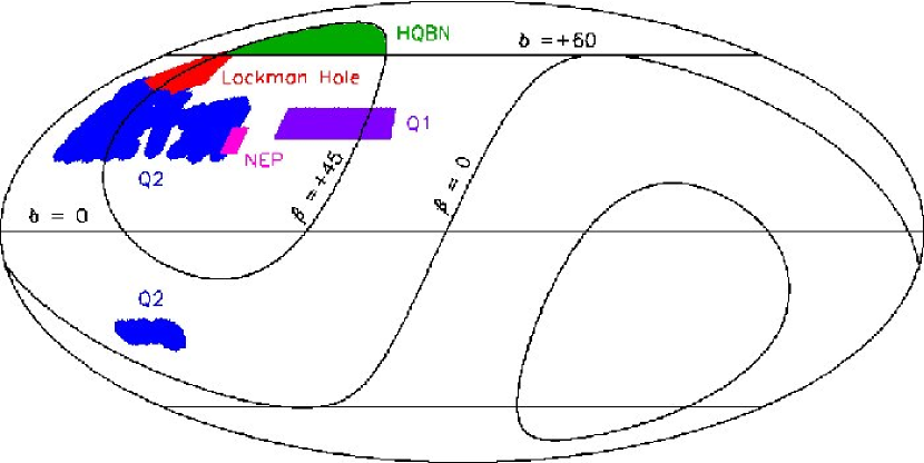
Figure 1: Location of the regions analyzed on a Galactic coordinate Mollweide projection centered at $l=0\arcdeg$. The Lockman Hole (LH) region is the region mapped in H I by Snowden et al. (1994). The north ecliptic pole (NEP) region is the region mapped in H I by Elvis, Lockman and Fassnacht (1994). The DIRBE high quality B north (HQBN) region is defined as the region at Galactic latitude $b>+60\arcdeg$ and ecliptic latitude $\beta>+45\arcdeg$. The first quadrant (Q1) region is defined by $30\arcdeg<l<80\arcdeg,30\arcdeg<b<41\arcdeg$. The second quadrant (Q2) region is a region previously studied by Lagache et al. (2000).

The regions of the sky analyzed in this paper are shown in Figure 1. Three of them were previously analyzed by Hauser et al. (1998) and Arendt et al. (1998): the Lockman Hole (LH), a 300 square degree region around the position of lowest H I column density at $l=152\arcdeg,b=+52\arcdeg$; an $8\arcdeg\times 9\arcdeg$ region centered on the north ecliptic pole (NEP) at $l=96\arcdeg,b=+30\arcdeg$; and the DIRBE high quality B north (HQBN) region at $b>+60\arcdeg$ and $\beta>+45\arcdeg$. These regions were originally selected because they were expected to have relatively weak Galactic and interplanetary dust foregrounds, and because good quality H I observations were available for them. The DIRBE high quality B south region is not included in our analysis because it is below the declination limit of the WHAM Northern Sky Survey. In addition, we analyze the second quadrant region previously studied by Lagache et al. (2000) and a new region in the first quadrant at $30\arcdeg<l<80\arcdeg,30\arcdeg<b<41\arcdeg$. We refer to these as the Q2 region and Q1 region, respectively. The Q2 region was originally selected because preliminary WHAM H$\alpha$ data were available for it. The Q1 region was selected because it is comparable to the Q2 region in Galactic latitude, it is at ecliptic latitude greater than 30 degrees, it has no molecular clouds detected in the CO survey of Hartmann, Magnani, and Thaddeus (1998), and it has no cold infrared excess features that are characteristic of molecular clouds in the 100 $\micron$ infrared excess map of Reach et al. (1998).

The datasets used in our analysis are listed in Table 1. We use DIRBE 60, 100, 140, and 240 $\micron$ mission-averaged skymaps from which the interplanetary foreground emission has been subtracted using the model of Kelsall et al. (1998). Foreground Galactic stellar emission is negligible at these wavelengths (Hauser et al. 1998, Arendt et al. 1998) and has not been subtracted from the data.

We use H I 21-cm line data integrated over a velocity range that includes all significant Galactic emission, converted to H I column density $N$(H I) assuming that the line emission is optically thin. The H I data for the LH and NEP regions are from Snowden et al. (1994) and Elvis, Lockman, and Fassnacht (1994), and were corrected for stray radiation using the AT&T Bell Laboratories H I survey (Stark et al. 1992). Estimated 1$\sigma$ uncertainties in $N$(H I) for these regions range from $0.5\times 10^{19}$ cm^-2 to $1.0\times 10^{19}$ cm^-2. The H I data that we use for the other regions are from the Leiden-Dwingeloo H I survey (Hartmann and Burton 1997), which has also been corrected for stray radiation (Hartmann et al. 1996). We adopt a 1$\sigma$ uncertainty of $1.25\times 10^{19}$ cm^-2 for each position in these regions. This is the uncertainty of the stray radiation correction that was estimated by Hartmann et al. (1996) for a reference position in the Lockman Hole region.

We use H$\alpha$ total intensity data from the Wisconsin H-Alpha Mapper (WHAM) Northern Sky Survey (Haffner et al. 2003), which covers the sky north of declination $-30\arcdeg$. The WHAM instrument has a 1 degree diameter field of view, and the survey was made on a regular Galactic coordinate grid with pointings separated by $0.98\arcdeg/$cos $b$ in $l$ and $0.85\arcdeg$ in $b$. The spectrum for each pointing was integrated over $-80<v_{LSR}<80$ km s^-1 to obtain total H$\alpha$ intensity. For the regions we study, systematic errors associated with removal of geocoronal and atmospheric emission lines from the spectra can be greater than statistical measurement uncertainties. These errors can vary from night to night, and sometimes cause $\sim 7\arcdeg\times 7\arcdeg$ ”blocks” of data taken on particular nights to be noticeably offset in mean intensity relative to their surroundings. We applied offset corrections to affected blocks in the HQBN, Lockman Hole, and Q2 regions to remove discontinuities in H$\alpha$ intensity at the block boundaries. For the HQBN and Q2 regions, most blocks appeared to be unaffected and these were assumed to set the zero level of the data. For the HQBN region, an offset of 0.15 Rayleigh was added to the data in the areas ($102\arcdeg<l<117\arcdeg,65\arcdeg<b<71\arcdeg$), ($60\arcdeg<l<90\arcdeg,65\arcdeg<b<71\arcdeg$), and ($l>117\arcdeg,60\arcdeg<b<65\arcdeg$). For the Q2 region, an offset of 0.3 R was added in ($129\arcdeg<l<136.6\arcdeg,41\arcdeg<b<47\arcdeg$) and an offset of 0.4 R was added in ($136\arcdeg<l<157\arcdeg,47\arcdeg<b<51\arcdeg$). For the Lockman Hole, the offset corrections are somewhat uncertain and subjective since many blocks appear to be affected, by varying amounts. Offset corrections ranged from -0.5 to 0.1 R, and the zero level is determined by the WHAM observations of Hausen et al. (2002) for two positions in the region. Our decomposition results for the Lockman Hole are consistent with those for the other regions, and omitting this region from our analysis does not change our derived CIB results significantly. We adopt a 1$\sigma$ uncertainty of 0.06 Rayleigh for the velocity-integrated, offset-corrected H$\alpha$ intensity at each WHAM pointing. This is near the low end of the range of rms H$\alpha$ dispersion measured within observing blocks at high Galactic latitudes. The dispersion tends to increase with increasing mean H$\alpha$ intensity or decreasing latitude, presumably due to increasing rms dispersion in Galactic emission. With the adopted uncertainty, the mean H$\alpha$ signal-to-noise ratio is 4, 8, 18, 18, and 31 for the LH, HQBN, Q1, Q2, and NEP regions, respectively.

The DIRBE data and Leiden H I data were interpolated to the WHAM pointing positions for our analysis. The angular resolution of the Elvis et al. and Snowden et al. H I data is much better that that of the other datasets, so these data were averaged over the WHAM field of view at each WHAM pointing position. Possible contamination by stellar H$\alpha$ absorption was handled either by excluding positions with stars brighter than $V=6.5$, or by excluding positions with H$\alpha$ intensity significantly lower than their surroundings. These two methods were compared for the LH and NEP regions, and found to give consistent results. Some positions with a discrete source detected in the DIRBE data (the planetary nebulae NGC 6543, and galaxies NGC 3079, 3310, 3556, 3690, and 4102) were excluded from our analysis. The planetary nebula NGC 6210 appears as a bright point source in the WHAM data (Reynolds et al. 2005) and was also excluded.

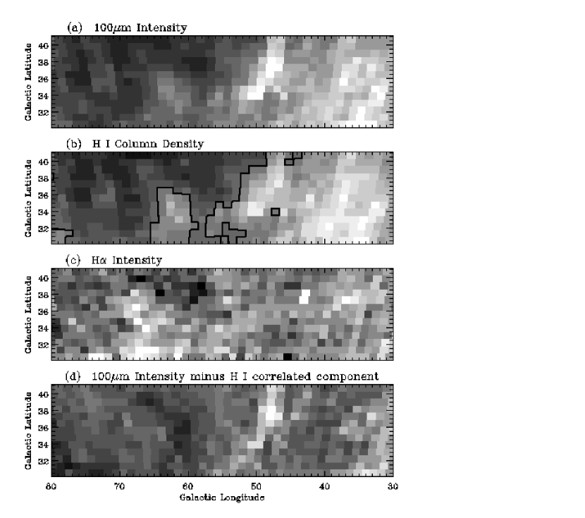
Figure 2: Images of the Q1 region in (a) DIRBE 100 $\micron$ intensity after subtraction of the interplanetary dust emission model, (b) H I column density from the Leiden-Dwingeloo survey, (c) H$\alpha$ intensity from the WHAM Northern Sky Survey, and (d) 100 $\micron$ intensity as in (a) but with the component that is correlated with H I column density subtracted. The distributions of H I and H$\alpha$ differ from each other and differ from an isotropic distribution, so the infrared data can be decomposed into a sum of the three distributions. No correlation is seen between H$\alpha$ and the residual 100 $\micron$ emission in (d), consistent with the low value of the H$\alpha$ coefficient $B_{1}$ obtained from our analysis. Possibly the 100 $\micron$ emissivity of the ionized medium is low and the intensity variations in (d) are not related to the ionized medium, or H$\alpha$ is not a good tracer of the 100 $\micron$ emission from this medium. The image display ranges, from black to white, are 20 to 170 nW m^-2 sr^-1 for (a), 0.4 to 6.3 10²⁰ atoms cm^-2 for (b), 0.5 to 1.6 R for (c), and -25 to 50 nW m^-2 sr^-1 for (d). The black contour in (b) shows the N(H I) cut of 3 10²⁰ atoms cm^-2 used in the analysis, as described in §3.1.

Maps of the 100 $\micron$ intensity, H I column density, and H$\alpha$ intensity are shown for the Q1 region in Figure 2, and correlation plots are shown for this region in Figure 3. These figures show that the correlation between $\nu I_{\nu}$(100 $\micron$) and $N$(H I) is tighter than that between $\nu I_{\nu}$(100 $\micron$) and $I$(H$\alpha$) or that between $I$(H$\alpha$) and $N$(H I). Similar trends are seen for the other regions analyzed in this paper, and for the region around $l=144\arcdeg,b=-21\arcdeg$ studied previously (Reynolds et al. 1995, Arendt et al. 1998).

3 Analysis

3.1 Decomposition of the Infrared Emission

The method of analysis follows that used by Arendt et al. (1998) and is similar to that used by Lagache et al. (2000). For each DIRBE wavelength band (60, 100, 140, and 240 $\micron$), the infrared intensity distribution within a given region is decomposed into a component that is correlated with H I column density, a component that is correlated with H$\alpha$ intensity, and an isotropic component. This is done by making a least squares fit of the form

$$\nu I_{\nu}(\lambda)=A_{1}N({\rm H\,I})+B_{1}I(\rm H\alpha)+\it C_{1}$$ (1)

where $I_{\nu}(\lambda)$ is the infrared intensity after interplanetary foreground subtraction and $A_{1}$, $B_{1}$, and $C_{1}$ are fit parameters. $A_{1}$ is the mean infrared emissivity per H atom for dust in the neutral atomic gas phase, $B_{1}$ is a measure of the mean infrared emissivity of dust in the ionized gas phase, and the intercept $C_{1}$ is the mean residual infrared intensity. For comparison, a second decomposition is performed in which an H$\alpha$ correlated component is not included, by making a fit of the form

$$\nu I_{\nu}(\lambda)=A_{2}N({\rm H\,I})+C_{2}.$$ (2)

Comparison of the derived $C_{1}$ and $C_{2}$ values gives the error in the Galactic foreground subtraction if the H$\alpha$ correlated component is neglected.

Decomposition of an infrared intensity distribution into three components as in equation (1) will be successful if the spatial distibutions of $N$(H I) and $I$(H$\alpha$) differ significantly from each other, and also differ significantly from an isotropic distribution. These conditions are met for each of the regions studied here. This is illustrated for the Q1 region by Figures 2 and 3. The method of analysis also assumes that H$\alpha$ intensity is a good tracer of far infrared emission from the ionized medium. In §5, we discuss possible errors in our results if this is not the case. Extinction of the H$\alpha$ emission is another potential source of error, but its effect is negligible for our regions with the data selection criteria described below. We made fits to the 100 $\micron$ data for each region with and without a correction to $I$(H$\alpha$) for extinction, and differences in the results were insignificant. We made the worst-case assumption of pure foreground extinction. With the optical depth at H$\alpha$ calculated as $\tau=0.04[N$(H I)/$10^{20}$ cm^-2], the extinction correction was at most 1.22.

The fits are made using an iterative procedure that minimizes $\chi^{2}$ calculated using measurement uncertainties in the independent and dependent variables (Press et al. 1992). Uncertainties in the fit parameters are determined from the 68% joint confidence region in parameter space, using the method of Bard (1974). For each of the regions except for HQBN, data at the highest H I column densities are excluded from the fitting, as described by Arendt et al. (1998) for the LH and NEP regions. The $\nu I_{\nu}(100\thinspace\micron)$ – N(H I) relation deviates from linearity in these regions, with excess 100 $\micron$ emission relative to N(H I) at the highest H I column densities. This type of relation has been found previously for isolated cirrus clouds and for large regions of the sky at high Galactic latitude, and the excess 100 $\micron$ emission has been attributed to emission from dust associated with molecular gas or to non-negligible optical depth in the 21-cm line (e.g., Deul and Burton 1993, Reach, Koo, and Heiles 1994, Boulanger et al. 1996). For the Lockman Hole, it is consistent with detections of CO line emission toward some 100 $\micron$ brightness peaks (Heiles, Reach, and Koo 1988; Stacy et al. 1991; Reach, Koo, and Heiles 1994). We exclude data above H I column densities where the $\nu I_{\nu}(100\thinspace\micron)$ – N(H I) relation begins to deviate from linearity (see Figure 8 of Arendt et al. 1998). The cut is made at $N({\rm H\,I})=1.5\times 10^{20}$ cm^-2, $5.0\times 10^{20}$ cm^-2, $3.0\times 10^{20}$ cm^-2, and $3.0\times 10^{20}$ cm^-2 for the LH, NEP, Q1, and Q2 regions, respectively. Measurement uncertainties are much larger for the DIRBE 140 and 240 $\micron$ bands than for the 60 and 100 $\micron$ bands, so less stringent N(H I) limits were adopted for the LH and NEP fits in these bands, $2.0\times 10^{20}$ cm^-2 for the LH and $6.0\times 10^{20}$ cm^-2 for the NEP. With these cuts, the area of the sky used in the 100 $\micron$ analysis is 420, 170, 35, 180, and 380 square degrees for the HQBN, LH, NEP, Q1, and Q2 regions, respectively.

3.2 Limits on Emission from Dust in H₂

Our analysis does not allow for possible FIR emission from molecular gas that is not correlated with H I. This emission is expected to be negligible for the WHAM pointings that pass the $N$(H I) cuts. Gillmon et al. (2006) and Gillmon and Shull (2006) reported results from a FUSE survey of H₂ absorption lines toward 45 AGNs at $|b|>20\arcdeg$. They compared their derived values of the molecular fraction, $f_{H_{2}}=2N($H${}_{2})/[N($H I$)+2N($H${}_{2})]$, with values of temperature-corrected 100 $\micron$ intensity $D^{T}$ from the map of Schlegel, Finkbeiner, and Davis (1998). ($D^{T}$ is proportional to Galactic dust column density.) The transition from low molecular fractions characteristic of optically thin clouds to high values characteristic of H₂ self-shielded clouds was found to occur over the range $1.5<D^{T}<3$ MJy sr^-1, with $f_{H_{2}}$ varying between $10^{-6}$ and $10^{-1}$ in this $D^{T}$ range, $f_{H_{2}}$ less than $10^{-3}$ at lower $D^{T}$ values, and $f_{H_{2}}$ between $10^{-2}$ and 0.3 at higher $D^{T}$ values. Except for the NEP region, most of the WHAM pointings used in our analysis (after the $N$(H I) cuts have been applied) have $D^{T}$ less than 1.5 MJy sr^-1, so $f_{H_{2}}$ is expected to be generally less than $10^{-3}$ and the uncertainty in derived CIB results due to neglect of this component is negligible. For each region except the NEP, we estimate that dust associated with H₂ contributes less than 0.04, 0.05, and 0.02 nW m^-2 sr^-1 at 100, 140, and 240 $\micron$, respectively. This assumes that $N$(H₂) is constant within a region, $2N$(H${}_{2})<10^{-3}\thinspace\times$ mean $N$(H I), and IR emissivity per H nucleus in the H₂ phase is given by the slope of the IR – $N$(H I) relation. For the NEP, most of the WHAM pointings that are used have $D^{T}$ in the transition range from 1.5 to 3.0 MJy sr^-1, so $f_{H_{2}}$ values as large as 0.1 are possible. However, we find no evidence for significant IR emission from H₂ associated dust. The mean residual infrared intensities $C_{1}$ from our analysis of the NEP region are consistent with the values found for the other regions, and the 100 $\micron$ – $N$(H I) relation for the NEP is linear with small scatter over the range of $N$(H I) used in our analysis (see figures 7 and 8 of Arendt et al. 1998). Excluding the NEP region from our analysis would not change our derived CIB results significantly.

3.3 Test Against Previous Results

As a check of our analysis method and software, we performed fits of the form of equation (1) using data previously analyzed by Lagache et al. (2000) for the Q2 region. Lagache et al. performed fits of this form for 122 positions in the region using DIRBE data with interplanetary foreground subtracted, Leiden-Dwingeloo H I data, and preliminary WHAM data, all smoothed to the $\sim 7\arcdeg$ resolution of the COBE/FIRAS. They kindly provided us with the data. We performed fits as described above, except to be consistent with the Lagache et al. analysis, only measurement uncertainties for the dependent variable (the infrared intensity) were used in the calculation of $\chi^{2}$. Table 2 gives a comparison of our results and the Lagache et al. results. The two analyses give the same values for the fit parameters, but the values for the fit parameter uncertainties do not agree. Our uncertainties for $A_{1}$ and $B_{1}$ are larger than those given by Lagache et al. because our uncertainty calculation allows for uncertainty due to coupling between the parameters. (The uncertainty quoted for $C_{1}$ by Lagache et al. is not a statistical uncertainty from the fitting, but was determined from the distribution of residual intensity values, so comparison with our uncertainty value for $C_{1}$ is not meaningful.) We conclude from this test that differences between our results in §4 and those of Lagache et al. are not the result of software errors.

4 Results

Parameters from our fits for the five regions are listed in Table 3. Positions with H I column density greater that the cuts described in section 3.1 were excluded from the fitting. For each region and each wavelength, the first row in the table gives results from the three-component fit (equation 1) and the second row gives results from the two-component fit (equation 2). The uncertainties listed are statistical uncertainties from the 68% joint confidence region in parameter space; the $C_{1}$ and $C_{2}$ uncertainties do not include systematic uncertainties that need to be included in determining the total uncertainty for a CIB measurement. Column 7 of the table lists the number of independent WHAM pointings used for each fit. Sample correlation plots showing the fits to the 100 $\micron$ data for the Q1 and Q2 regions are shown in Figure 4, and parameters from the three-component fits for each region are plotted as a function of wavelength in Figures 5 and 6.

For all regions in all wavelength bands analyzed, we find that the mean residual intensity is nearly the same whether an H$\alpha$-correlated component is included in the fitting or not (the $C_{1}$ and $C_{2}$ values are in close agreement), and the quality of the fit is nearly the same in the two cases. Also, we do not detect significant H$\alpha$-correlated infrared emission; the $B_{1}$ values are consistent with zero within the uncertainties, and the $A_{1}$ and $A_{2}$ values are nearly the same. The lack of H$\alpha$-correlated 100 $\micron$ emission is illustrated for the Q1 region in Figures 2 and 3. No correlation is seen between the H$\alpha$ map in Figure 2c and and the map in Figure 2d of residual 100 $\micron$ emission after subtraction of H I correlated 100 $\micron$ emission. This is also shown by the correlation plot in Figure 3d.

4.1 Residual Intensities and CIB Measurements

Figure 7 shows the residual intensity averaged over the five regions as a function of wavelength for each fit type; the $C_{1}$ and $C_{2}$ values were each averaged over the regions using weighting by 1/$\sigma^{2}$. The weighted-average residual intensities for the different fit types agree within 1$\sigma$ statistical uncertainties at all wavelengths, and the agreement is within 2 nW m^-2 sr^-1 at 60, 100, and 240 $\micron$. We conclude that addition of an H$\alpha$-correlated component in modeling the foreground emission at high Galactic latitude has negligible effect on derived CIB results.

To assess whether the weighted-average values for the residual emission can be identified as CIB measurements, we calculated the total uncertainty for these values following the method used by Hauser et al. (1998). The total uncertainty was calculated as the quadrature sum of the statistical uncertainty, interplanetary foreground subtraction uncertainty, and DIRBE detector offset uncertainty. Magnitudes of the latter two uncertainties were taken from Table 6 of Arendt et al. (1998). (DIRBE gain uncertainty is not included because it has the same multiplicative effect on the mean residual and its total uncertainty, and so does not affect the signal-to-noise ratio. This uncertainty is 10–14% for the DIRBE bands used here.) Based on these total uncertainties, the mean residual emission is more than 3$\sigma$ greater than zero at 140 $\micron$ and 240 $\micron$ for both the two-component fits and the three-component fits, and at 100 $\micron$ for the three-component fits. The residual intensity values for the five different regions (Table 3 and Figure 6) are consistent with isotropy at 140 $\micron$ and 240 $\micron$ (the values are compatible within their 1$\sigma$ uncertainties). We have not performed detailed anisotropy tests on the maps of residual intensity from our analysis, such as the tests performed by Hauser et al. (1998). However, based on the reduced chi-square values in Table 3, significant anisotropy is present in the Q1 and Q2 regions at 60 $\micron$ and in all five regions at 100 $\micron$.

Table 4 lists the upper limits and detections of the CIB at 60, 100, 140, and 240 $\micron$ from Hauser et al. (1998), from our two-component and three-component fits, and from Lagache et al. (2000). For cases where the mean residual intensity does not exceed zero by greater than 3$\sigma$ or the residual intensity distribution has been shown to be anisotropic, the table lists a 2$\sigma$ upper limit on the CIB followed by the mean residual intensity and its 1$\sigma$ uncertainty in parentheses. Our results are consistent with those of Hauser et al. Our residuals have not passed a detailed anisotropy test, and in some cases our quoted uncertainties are slightly larger than those of Hauser et al., so our CIB results do not supersede the Hauser et al. results.

If H$\alpha$ intensity is not a good tracer of infrared emission from dust in the WIM, our three-component fits may not account for emission from the WIM much better than fits without an H$\alpha$ correlated component do. Any emission from the WIM that is not correlated with H$\alpha$ or H I would contribute to the residual component, so our results would overestimate the CIB. The agreement with the Hauser et al. (1998) results could be because their analysis overestimates the CIB by a similar amount. In §5.4 we discuss evidence that H$\alpha$ may not be a good tracer, and we estimate the possible effect of emission from the WIM on the CIB results from our analysis and from that of Hauser et al. For each analysis, we estimate the effect to be only about 5% at 140 and 240 $\micron$, which is much smaller than the quoted uncertainties.

4.1.1 Systematic Uncertainties

Although this paper is primarily concerned with the effect of the ionized ISM on CIB determination, we discuss here other systematic uncertainties involving the level of the H I cut, choice of interplanetary dust model, and choice of photometric calibration. Our results for the effect of the ionized ISM have no significant dependence on any of these uncertainties.

Arendt et al. (1998) found that the sensitivity of the Hauser et al. (1998) CIB results to the H I cut is negligible compared to other sources of uncertainty. For the Lockman Hole, for example, the mean 100 $\micron$ residual intensity was found to vary by less than 0.7 nW m^-2 sr^-1 when the cut was varied from 1.0 to $2.0\times 10^{20}$ cm^-2. We have investigated the sensitivity of the CIB results from our three-component analysis to the H I cut used for our regions that were not included in the Hauser et al. analysis, the Q1 and Q2 regions. The effect of varying the cut for these regions over the range from 2.5 to $3.5\times 10^{20}$ cm^-2 is small. The derived mean residual changes by +0.1, -0.7, -0.1, and +0.7 nW m^-2 sr^-1 at 60, 100, 140, 240 $\micron$, respectively, when the cut is changed from 3.0 to $2.5\times 10^{20}$ cm^-2. These changes are at most 25% of the uncertainties of the mean residuals given in Table 4. The mean residual changes by -0.8, -0.5, -3.0, and -1.3 nW m^-2 sr^-1 in these bands when the cut is changed from 3.0 to $3.5\times 10^{20}$ cm^-2. These changes are at most 45% of the quoted uncertainties of the mean residuals.

The effect of choice of interplanetary dust model is shown in Table 5. This table compares mean residual intensities from Hauser et al. (1998) with those obtained by Wright (2004). The main difference between these analyses is that Hauser et al. used the interplanetary dust model of Kelsall et al. (1998) and Wright used the model of Gorjian et al. (2000). Each of these models was obtained by fitting the time variation observed over the whole sky in each of the DIRBE bands with a parameterized model of the dust cloud, but Gorjian et al. added a constraint that the residual 25 $\micron$ intensity after zodiacal light subtraction be zero at high Galactic latitude. This assumed that the 25 $\micron$ CIB is negligible, based on CIB upper limits inferred from TeV gamma ray observations of Mrk 501. Table 5 also lists the uncertainty of the zodiacal light subtraction for the Hauser et al. analysis, as estimated by Kelsall et al. This was obtained by comparing results from a series of models with different geometries for the density distribution of the dust cloud, which gave comparable quality fits to the time variation of the DIRBE data. The difference between the Hauser et al. results and the Wright results is not significant relative to the uncertainty in zodiacal light subtraction, or relative to the total uncertainty of the mean residual.

Hauser et al. (1998) noted the effects on CIB results at 140 and 240 $\micron$ if the DIRBE data are transformed to the FIRAS photometric system. The CIB values are affected by differences in zero point and gain between the DIRBE and FIRAS photometric systems, which are not significant relative to the zero point uncertainties and gain uncertainties for the two systems. Hauser et al. found that transforming the DIRBE CIB results to the FIRAS system would reduce the CIB value from 25.0 to 15.0 nW m^-2 sr^-1 at 140 $\micron$, and from 13.6 to 12.7 nW m^-2 sr^-1 at 240 $\micron$. The DIRBE team chose to use the DIRBE photometric system to report its results since comparing the two photometric systems has its own uncertainties associated with the need to integrate the DIRBE map over the FIRAS beam, and the FIRAS spectrum over the DIRBE spectral response. The DIRBE team chose not to introduce this additional uncertainty, and we made the same choice for this paper.

4.1.2 Comparison with Spitzer Source Counts

Recently, Dole et al. (2006) used Spitzer MIPS observations to measure the contribution of galaxies selected at 24 $\micron$ to the CIB at 70 $\micron$ and 160 $\micron$. They found that sources brighter than 60 $\mu$Jy at 24 $\micron$ contribute 5.9 $\pm$ 0.9 and 10.7 $\pm$ 1.6 nW m^-2 sr^-1 to the CIB at 70 $\micron$ and 160 $\micron$, respectively. With an extrapolation of the 24 $\micron$ source counts below the 60 $\mu$Jy detection threshold, they estimated that the full population of 24 $\micron$ sources contributes 7.1 $\pm$ 1.0 and 13.4 $\pm$ 1.7 nW m^-2 sr^-1 at 70 and 160 $\micron$. They noted that these should be regarded as lower limits to the CIB since there may be contributions from a diffuse background component or from sources missed by the 24 $\micron$ selection. They estimated that these contributions account for less than $\sim 20\%$ of the far infrared CIB.

A diffuse component of the CIB could be produced by processes such as emission from intergalactic dust or radiative decay of primordial particles. Here we compare the Dole et al. integrated galaxy brightness at 160 $\micron$ with DIRBE CIB measurements at 140 $\micron$ and 240 $\micron$ to estimate upper limits on emission from a diffuse component. We scale the quoted 160 $\micron$ intensity of 13.4 $\pm$ 1.7 nW m^-2 sr^-1 to 140 $\micron$ and 240 $\micron$ using the shape of the model spectral energy distribution from figure 13 of Dole et al., which is based on the Lagache et al. (2004) galaxy evolution model. This spectrum is also used to apply color corrections so the intensities can be compared with the quoted DIRBE CIB values, which assume a spectral shape of $\nu I_{\nu}=$ constant over the DIRBE bandpass. We obtain integrated galaxy intensity values of 13.7 $\pm$ 1.7 nW m^-2 sr^-1 at 140 $\micron$ and 10.7 $\pm$ 1.4 nW m^-2 sr^-1 at 240 $\micron$. The uncertainties here do not include any uncertainty in the shape of the adopted spectral energy distribution. Table 6 compares these values with the DIRBE CIB results, and with DIRBE CIB results transformed to the FIRAS photometric system (Hauser et al. 1998). The table lists values for the fractional contribution of the integrated galaxy brightness to the CIB, and the difference between the CIB and the integrated galaxy brightness. Using the CIB results on the DIRBE photometric system yields 2$\sigma$ upper limits for a diffuse CIB component of 26 nW m^-2 sr^-1 at 140 $\micron$ and 8.5 nW m^-2 sr^-1 at 240 $\micron$.

4.2 Infrared Emissivity of the Ionized Medium

Infrared emissivity results from our three-component fits are shown as a function of wavelength in Figure 5. The derived values of emissivity per H atom for the neutral atomic gas phase, $\epsilon$(H⁰), are comparable to previous determinations from high latitude IR – H I correlation studies (e.g., Dwek et al. 1997, Reach et al. 1998). The values of emissivity per H⁺ ion for the ionized phase, $\epsilon$(H⁺), were obtained from the $B_{1}$ values in Table 3 using a conversion factor of $I$(H$\alpha$)/$N$(H${}^{+})$ = 1.15 Rayleighs/$10^{20}$ cm^-2. This is the mean ratio of H$\alpha$ intensity to pulsar dispersion measure found by Reynolds (1991b) for four high latitude lines of sight toward pulsars at $z>$ 4 kpc. It corresponds to an effective electron density, $n_{eff}\equiv\int n_{e}^{2}ds/\int n_{e}ds$, of 0.08 cm^-3 for an electron temperature of 8000 K and no extinction. The $I$(H$\alpha$)/$N$(H${}^{+})$ ratio ranges from 0.75 to 1.9 Rayleighs/$10^{20}$ cm^-2 for the lines of sight studied by Reynolds, so the uncertainty in the conversion factor is large. The value adopted here is the same as that used by Lagache et al. (2000). Figure 5 shows that the derived values of $\epsilon$(H⁺) are consistent with zero for all regions at all wavelengths. We have checked the dependence of derived 100 $\micron$ $\epsilon$(H⁺) values on the H I cut, and find that they do not change significantly when the cut is varied by $\pm$ 30%.

Our derived values of $\epsilon$(H⁺) at 100 $\micron$ are compared with previous results for other regions of the sky in Table 7. All of the results listed are from analyses similar to that used here, with either H$\alpha$ intensity or centimeter wavelength radio continuum intensity used as the tracer of the ionized gas. Column 4 lists the electron density adopted in each study for calculating the conversion from H$\alpha$ or radio continuum intensity to $N$(H⁺). Uncertainty in this conversion may be as large as a factor of two or more for some regions, but is not included in the uncertainty listed for $\epsilon$(H⁺). The emissivity values are shown plotted as a function of electron density in Figure 8. The 2$\sigma$ upper limits for our regions are comparable to that obtained by Arendt et al. (1998) for the $10\arcdeg\times 12\arcdeg$ region at $l=144\arcdeg,b=-21\arcdeg$. For the other previously studied regions, 100 $\micron$ emission was detected from the ionized gas component, and the derived $\epsilon$(H⁺) is greater than or equal to the 100 $\micron$ $\epsilon$(H⁰). This can be explained if the dust-to-gas mass ratio is the same in the ionized and neutral atomic components, with cases of enhanced emissivity in the ionized component caused by Lyman alpha heating (for the Barnard’s Loop region, Heiles et al. 2000) or a local source of heating (for the Spica region, Boulanger et al. 1995, Zagury, Jones, and Boulanger 1998), or both (for the Galactic plane regions, Sodroski et al. 1997). With the exception of the Q2 region, the ionized gas in these regions is not representative of the general warm ionized medium observed at high latitudes. The electron density is an order of magnitude greater, and the ionized gas is much closer to the Galactic midplane ($z<$ 100 pc, compared to an exponential $z$ scale height of about 900 pc for the warm ionized medium (Reynolds 1993)).

The 100 $\micron$ $\epsilon$(H⁺) value determined by Lagache et al. (2000) for the Q2 region without an H I cut is not consistent with our result for the Q2 region with an H I cut applied, or with results for the other high latitude regions that sample the general warm ionized medium. We have applied our three-component decomposition to the full Q2 region (with no H I cut) at 100 $\micron$ at the 1 degree resolution of the WHAM data. This gave $\epsilon$(H⁺) = 8.5 $\pm$ 1.0 nW m^-2 sr^-1/$10^{20}$ cm^-2, which is comparable to the upper limits in figure 8, and $\epsilon$(H⁰) = 18.7 $\pm$ 0.4 nW m^-2 sr^-1/$10^{20}$ cm^-2. (If an extinction correction is applied to the H$\alpha$ data as described in §3.1, the derived $\epsilon$(H⁺) is 5.5 $\pm$ 1.0 nW m^-2 sr^-1/$10^{20}$ cm^-2.) The difference between these results and those of Lagache et al. is probably due to the different angular resolution used. Their analysis used data for 122 positions at 7 degree FIRAS resolution, but the data were oversampled and there are only about 30 independent FIRAS pointings within the region. Our analysis used data for 1762 independent WHAM pointings that are within 3.5 degrees (half of the FIRAS beam width) of any of their 122 positions. It is possible that some unmodeled effect, such as dust associated with molecular gas, optical depth in the 21-cm line, or variation of $\epsilon$(H⁰), happens to correlate with the H$\alpha$ data at FIRAS resolution, but does not correlate as well at WHAM resolution. The $\nu I_{\nu}(100\micron)$ – N(H I) relation for the region shows curvature, which suggests that molecular gas or 21-cm line opacity may be present. We find that 40% of the region has temperature-corrected 100 $\micron$ intensity greater than the 3 MJy sr^-1 threshold for significant fractional H₂ abundance (Gillmon and Shull 2006). For these reasons, we consider the emissivity per H⁺ ion derived for the full Q2 region, from either our analysis or Lagache et al.’s analysis, to be of questionable reliability.

5 Discussion

Our derived emissivity values for the ionized medium are statistically consistent with zero. From Table 7, our derived 2$\sigma$ upper limits on 100 $\micron$ emissivity per H⁺ ion are 0.33, 1.11, 0.37, 0.57, and 0.30 of the 100 $\micron$ emissivity per H atom for the HQBN, LH, NEP, Q1, and Q2 regions, respectively. We adopt 0.4 as a representative upper limit on $\epsilon($H${}^{+})/\epsilon($H${}^{0})$ at 100 $\micron$ for these regions. Possible explanations for this low value include a lower dust-to-gas mass ratio or a weaker radiation field in the ionized medium than in the neutral medium, a difference in grain optical properties or grain size distribution, an error in our adopted $I$(H$\alpha$)/$N$(H${}^{+})$ conversion factor, or a shortcoming of using H$\alpha$ as a tracer of infrared emission from dust in the ionized medium. In this section, we discuss some of these possibilities. Based on available observations and models, it appears that our low derived $\epsilon($H${}^{+})/\epsilon($H${}^{0})$ ratio is partly due to a lower dust-to-gas mass ratio in the WIM and partly due to error in using H$\alpha$ as a tracer, but one or more of the other factors may also contribute. We discuss possible implications for derived CIB results in §5.4.

5.1 Dust-to-gas Mass Ratio

A lower dust-to-gas mass ratio would be expected if the ionized gas in these regions has greater $z$ extent and lower density than the neutral gas, as is typical for the WIM in the solar vicinity (Reynolds 1991a). From interstellar absorption line observations, it has been inferred that abundances of heavy elements in the form of dust decrease with increasing $z$, and also decrease with decreasing gas density (e.g., Savage and Sembach 1996). Most of these studies have pertained to the neutral atomic medium, but from observations of Al III and S III absorption lines, Howk and Savage (1999) found evidence that about 60-70% of aluminum atoms in the WIM are in dust, compared to about 90% of Al in dust in H II regions at low $z$. This result is based on observations of two lines of sight that sample the WIM up to $z$ distances of 690 pc and 2800 pc, and four lines of sight through low density ($n_{e}\sim$ 0.2 to 4 cm^-3) H II regions at $z<$ 200 pc. Howk and Savage also noted that the dust phase Al abundance they obtained for the low $z$ H II regions is comparable to previous, somewhat uncertain determinations for the warm neutral medium at low $z$. Assuming that this low $z$ dust phase Al abundance is valid for the neutral atomic medium in the regions studied here, and that 100 $\micron$ emissivity per H nucleus varies in proportion to Al dust phase abundance, one would expect $\epsilon$(H⁺) to be about 20–30% lower than $\epsilon$(H⁰) at 100 $\micron$.Thus the Howk and Savage results suggest that the difference in dust abundance between the neutral and ionized components is not great enough to fully explain our derived upper limit on $\epsilon($H${}^{+})/\epsilon($H${}^{0})$. To confirm this, dust phase Al abundance determinations for additional lines of sight through the WIM would be of interest, as would calculations of the relation between Al dust phase abundance and 100 $\micron$ emissivity for dust grain models.

5.2 Interstellar Radiation Field

The lower 100 $\micron$ emissivity derived for the ionized medium could also be explained if it were subject to a weaker interstellar radiation field. Heating of dust by Lyman alpha is expected to be negligible at the electron density estimated for the WIM (Spitzer 1978, Heiles et al. 2000). Also, there are no early type stars that are close enough to the lines of sight through our regions to cause significant dust heating relative to that of the general interstellar radiation field. Models of the spatial distribution of the interstellar radiation field at visual and ultraviolet wavelengths predict that the mean intensity increases with increasing $z$ up to about 200 pc, as light from distant stars in the Galactic disk becomes less attenuated, and then decreases with further increase in $z$ due to geometrical dilution. Wakker and Boulanger (1986) used their model of the radiation field to calculate the expected 100 $\micron$ intensity of a diffuse cloud with a mixture of silicate and graphite grains. The intensity was calculated for different distances of the cloud along two high latitude lines of sight (toward $b=90\arcdeg$, and toward $l=180\arcdeg$, $b=60\arcdeg$). They found that the 100 $\micron$ intensity varies by less than $\pm$20% over the range in cloud height from $z=$ 0 – 1 kpc. Thus, it appears that the radiation field does not vary enough to explain our derived limit on $\epsilon($H${}^{+})/\epsilon($H${}^{0})$, even if all the H I gas were located near the maximum of the radiation field and all of the H II gas were at $z=$ 1 kpc.

5.3 $I$(H$\alpha$)/$N($H${}^{+})$ Conversion Factor

To change our derived upper limit on $\epsilon($H${}^{+})/\epsilon($H${}^{0})$ at 100 $\micron$ from 0.4 to 1.0, the adopted $I$(H$\alpha$)/$N($H${}^{+})$ conversion factor would need to be changed from 1.15 to 2.9 Rayleighs/$10^{20}$ cm^-2. This is significantly larger than the largest value of 1.9 Rayleighs/$10^{20}$ cm^-2 measured by Reynolds (1991b) for lines of sight to four pulsars at high $z$. Values obtained by Arendt et al. (1998) for an additional 5 pulsar lines of sight range from 0.8 to 1.2 Rayleighs/$10^{20}$ cm^-2. Thus, it appears that there is not an error in the adopted conversion factor value that is large enough to fully explain the low emissivity derived for the ionized medium.

Independent evidence that supports our adopted conversion factor comes from interstellar absorption line studies. Our adopted value corresponds to an effective electron density of 0.08 cm^-3. Electron density estimates from observations of absorption lines of excited C⁺ toward extragalactic objects and high $z$ stars are comparable to this. In the most extensive study to date, Lehner, Wakker, and Savage (2004) presented results for 43 such lines of sight at $|\thinspace b\thinspace|>30\arcdeg$. Most of the observed absorption line components are at low velocity. For these, they find a mean density of $\langle n_{e}\rangle=0.08\pm 0.04$ cm^-3 (1$\sigma$ dispersion). For the Intermediate Velocity Arch, they find $\langle n_{e}\rangle=0.03\pm 0.01$ cm^-3, probably lower because the gas is at higher $z$ ($\sim 1$ kpc). The derived n_e values are averages over C⁺ regions in both the warm ionized medium and the warm neutral medium, but Lehner et al. used WHAM H$\alpha$ data to estimate that at least 50% of the excited C⁺ column density originates in the WIM for an average line of sight.

5.4 H$\alpha$ as a Tracer of Infrared Emission

Our derived emissivity values and CIB results are subject to error if the WHAM H$\alpha$ data are not a good tracer of far infrared emission from the WIM in the regions we study. Far infrared intensity is proportional to dust column density, whereas H$\alpha$ intensity is proportional to the square of the ionized gas density integrated along the line of sight, $I$(H$\alpha$) $\propto T_{e}^{-0.92}\int n_{e}^{2}ds$, where $n_{e}$ is electron density and $T_{e}$ is electron temperature (Reynolds 1992). Thus errors would be expected in our results if the spatial variation of H$\alpha$ intensity for a region is caused more by differences in mean electron density or mean electron temperature for different lines of sight than by differences in ionized gas column density. The approximate csc $|b|$ dependence of high latitude WHAM data (Haffner et al. 2003) provides evidence that H$\alpha$ is a reasonable tracer of $N$(H⁺) on large angular scales, but this isn’t necessarily true on the scales within the regions studied here.

Haffner, Reynolds, and Tufte (1999) and Reynolds, Haffner, and Tufte (1999) have found evidence that variations in H$\alpha$ intensity may be largely due to variations in electron density, based on their observations of H$\alpha$, [N II] $\lambda$ 6583, and [S II] $\lambda$ 6716 line intensities in the region $123\arcdeg<l<164\arcdeg$, $-35\arcdeg<b<-6\arcdeg$, and previous observations of these lines in halos of edge-on galaxies. The [N II]/H$\alpha$ and [S II]/H$\alpha$ intensity ratios are observed to increase with increasing $z$, while the [S II]/[N II] ratio is nearly constant. Interpreting the variations in [N II]/H$\alpha$ as primarily due to variations in electron temperature, Haffner et al. and Reynolds et al. inferred $T_{e}$ values ranging from 6000 K to 11000 K, with temperature increasing as H$\alpha$ intensity decreases. They showed that this anticorrelation can be explained if variations in H$\alpha$ are largely due to variations in mean electron density, and a supplemental source of gas heating is present that dominates over photoionization at low density, causing temperature to increase with decreasing density. A number of possible supplemental heating mechanisms have been proposed, and Reynolds et al. estimate the heating rate that would be needed to explain the observations for each mechanism.

If H$\alpha$ is not a good tracer of ionized gas column density, our method of analysis tends to underestimate the infrared emissivity per H⁺ ion and overestimate the CIB. To show this, we consider a simple model in which the H$\alpha$ variation in a region is partly due to variation of $N$(H⁺) and partly due to variation of effective electron density $n_{eff}$,

$$\frac{I(\rm H\alpha)}{\langle I(\rm H\alpha)\rangle}=\frac{N(\rm H^{+})}{\langle N(\rm H^{+})\rangle}\frac{n_{eff}}{\langle n_{eff}\rangle}$$ (3)

where $\langle I(H\alpha)\rangle$, $\langle N($H${}^{+})\rangle$, and $\langle n_{eff}\rangle$ are averages over all lines of sight through the region. This assumes that electron temperature is constant, and $\langle N($H${}^{+})\enspace n_{eff}\rangle=\langle N($H${}^{+})\rangle\thinspace\langle n_{eff}\rangle$. We adopt

$$\frac{N(\rm H^{+})}{\langle N(\rm H^{+})\rangle}=\left[\frac{I(\rm H\alpha)}{\langle I(\rm H\alpha)\rangle}\right]^{p},$$ (4)

and

$$\frac{n_{eff}}{\langle n_{eff}\rangle}=\left[\frac{I(\rm H\alpha)}{\langle I(\rm H\alpha)\rangle}\right]^{1-p},$$ (5)

where $p$ is the fraction of the variation of log $I$(H$\alpha$) that is caused by variation of $N$(H⁺). We assume that, averaged over large angular scales, $N$(H⁺) and $I$(H$\alpha$) are directly proportional,

$$\langle N(\rm H^{+})\rangle=\langle I(\rm H\alpha)\rangle/\it c,$$ (6)

where $c$ is our adopted conversion factor of 1.15 Rayleighs/$10^{20}$ cm^-2. The infrared emissivity per H nucleus is assumed to be constant within each gas phase, so the infrared emission from each phase is proportional to its gas column density. The infrared emission from the ionized phase is

$$\nu I_{\nu}^{WIM}=\epsilon(\rm H^{+})\it N(\rm H^{+})=\epsilon(\rm H^{+})\langle\it I(\rm H\alpha)\rangle^{1-{\it p}}\it I(\rm H\alpha)^{\it p}/\it c.$$ (7)

Assuming the distributions of $N$(H I) and $I$(H$\alpha$) are uncorrelated, the H$\alpha$ coefficient $B_{1}$ that would be obtained from our decomposition is the mean slope of the $\nu I_{\nu}^{WIM}$ – $I$(H$\alpha$) relation. If the distribution of H$\alpha$ intensities is symmetric about the mean, this is given by

$$B_{1}=\left.\frac{d\thinspace\nu I_{\nu}^{WIM}}{d\thinspace I(\rm H\alpha)}\right|_{I(\rm H\alpha)\thinspace=\thinspace\langle I(\rm H\alpha)\rangle}=p\epsilon(\rm H^{+})/\it c$$ (8)

and the emissivity per H⁺ ion derived from the analysis underestimates the actual emissivity,

$$\epsilon_{derived}(\rm H^{+})=\it cB_{1}=p\epsilon(\rm H^{+}).$$ (9)

Thus, our derived limit $\epsilon$(H⁺)/$\epsilon$(H${}^{0})<0.4$ may be consistent with no real difference in emissivity between the ionized and neutral phases if only a small fraction of the H$\alpha$ variation in our regions is caused by variation of $N$(H⁺), i.e., if $p<0.4$ in the context of this simple model. Berkhuijsen, Mitra, and Müller (2006) have estimated $p=0.68\pm 0.04$ for the high latitude diffuse ionized gas, using pulsar dispersion measure data and WHAM H$\alpha$ data toward a sample of 157 pulsars at $|b|>5\arcdeg$ (see their Figure 7b). This result suggests that our low derived $\epsilon$(H⁺)/$\epsilon$(H⁰) is at least partly due to error in using H$\alpha$ as a tracer.

The overestimate of the CIB for our simple model is given by the intercept of a linear fit to the $\nu I_{\nu}^{WIM}$ – $I$(H$\alpha$) relation. To a good approximation, this intercept is given by

$$\Delta\thinspace(\nu I_{\nu})=\left.\nu I_{\nu}^{WIM}\right|_{I(\rm H\alpha)\thinspace=\thinspace\langle I(\rm H\alpha)\rangle}-B_{1}\langle I(\rm H\alpha)\rangle.$$ (10)

Using equations (6), (7), and (8), we obtain

$$\Delta\thinspace(\nu I_{\nu})=(1-p)\thinspace\epsilon(\rm H^{+})\thinspace\langle\it N(\rm H^{+})\rangle.$$ (11)

We have used this result to estimate the possible effect of emission from the WIM that is not correlated with H$\alpha$ or $N$(H I) on the CIB results derived from our three-component fits. We subtracted $\Delta\thinspace(\nu I_{\nu})$ offsets from the derived residual intensities $C_{1}$ for each region assuming $p=0.5\pm 0.5$, $\langle N($H${}^{+})\rangle$ = $\langle I($H$\alpha)\rangle$/(1.15 Rayleighs/$10^{20}$ cm^-2), and $\epsilon($H${}^{+})=(0.5\pm 0.5)\thinspace\epsilon($H${}^{0})$, using values of $A_{1}$ in Table 3 for $\epsilon($H${}^{0})$. For each wavelength, we then calculated the weighted average of the reduced residual intensity over the five regions, treating the $\pm 0.5$ uncertainties in $p$ and $\epsilon($H${}^{+})/\epsilon($H${}^{0})$ as additional independent sources of error. The resulting average residual intensities are $21\pm 27$, $17.0\pm 6.3$, $23.5\pm 8.5$, and $12.0\pm 2.9$ nW m^-2 sr^-1 at 60, 100, 140, and 240 $\micron$, respectively. At 140 and 240 $\micron$, these results are only 6% lower than the results from our three-component fits.

Equation (11) is the same as the expression for the CIB overestimate from a two-component fit (using H I without H$\alpha$) where $p$ is the fraction of $N$(H⁺) that is correlated with $N$(H I). Thus we can use the same procedure to estimate the possible effect of emission from the WIM that is not correlated with $N$(H I) on the CIB results of Hauser et al. (1998). We make the same assumptions as in the previous paragraph for $p$, $\langle N($H${}^{+})\rangle$, and $\epsilon($H${}^{+})$. The HQBS region included in the Hauser et al. analysis is below the declination limit of the WHAM survey, so for this region we used data from the Southern H-Alpha Sky Survey of Gaustad et al. (2001) as processed by Finkbeiner (2003). We find that the weighted-average residual intensities from the Hauser et al. analysis would be reduced to $20.9\pm 6.2$, $23.6\pm 7.0$, and $12.9\pm 2.5$ nW m^-2 sr^-1 at 100, 140, and 240 $\micron$, respectively. These results are only about 5% lower than those of Hauser et al.

The possible effect of the ionized medium is also estimated to be small for the 125-2000 $\micron$ CIB spectrum determined by Fixsen et al. (1998) from FIRAS observations. In one of their analyses, Galactic emission template maps were constructed from DIRBE 140 $\micron$ and 240 $\micron$ data with the Hauser et al. (1998) CIB and zodiacal light subtracted, and the CIB spectrum was obtained by correlating FIRAS data with these templates. Our estimate of $\sim 5$% for the possible error of the DIRBE CIB results also applies to the $140\thinspace\mbox{${}_{<}\atop{}^{\sim}$}\thinspace\lambda\thinspace\mbox{${}_{<}\atop{}^{\sim}$}\thinspace 240\thinspace\micron$ part of the CIB spectrum derived from this analysis. At longer wavelengths, the error is expected to decrease. This is because the spectrum of emission from the ionized medium is expected to be similar to the spectrum of emission from the H I phase, and the ratio of this spectrum to the CIB spectrum decreases with increasing wavelength for $\lambda>240\thinspace\micron$. Since all three of the Fixsen et al. analyses gave consistent results for the CIB spectrum, the possible error due to the WIM should be small for their average CIB spectrum from the three methods.

6 Summary

We used WHAM H$\alpha$ data as a tracer of far infrared emission from the warm ionized phase of the ISM in an effort to determine the intensity of this emission at high Galactic latitudes and to assess its effect on determination of the cosmic far infrared background. We studied five high latitude regions, including regions previously analyzed by Hauser et al. (1998) and Lagache et al. (2000). For each region, we decomposed COBE/DIRBE data at 60, 100, 140, and 240 $\micron$ into a sum of an H I correlated component, an H$\alpha$ correlated component, and a residual component. Uncertainties in our results due to omission of an H₂ correlated component are expected to be negligible, based on results of a FUSE high latitude H₂ absorption line survey. We found that the intensity of the H$\alpha$ correlated component is consistent with zero within the uncertainties for all regions at all wavelengths. From the mean intensities of the residual components, we derived estimates of the CIB at 140 and 240 $\micron$ and upper limits to the CIB at 60 and 100 $\micron$ (Table 4). We repeated the analysis without including an H$\alpha$ correlated component, and the derived CIB results did not change significantly. Our CIB estimates and upper limits are similar to previous CIB determinations for which the FIR emission from the ISM was traced only by H I column density. We conclude that addition of an H$\alpha$ correlated component in modeling the ISM emission at high Galactic latitude has negligible effect on derived CIB results. We did not perform detailed anisotropy tests on the maps of residual intensity from our analysis, so our CIB results do not supersede the results of Hauser et al. (1998).

We derived 2$\sigma$ upper limits to the 100 $\micron$ emissivity per H⁺ ion for the five regions that are typically about 40% of the emissivity per H atom for the neutral atomic medium. Available evidence suggests that this low value is partly due to a lower dust-to-gas mass ratio in the ionized medium than in the neutral atomic medium, and partly due to a shortcoming of using H$\alpha$ as a tracer of FIR emission, which causes our analysis to underestimate the emissivity of the ionized medium. Other possible effects that may play a role include a weaker radiation field in the ionized medium than in the neutral medium, a difference in grain optical properties or grain size distribution, or an error in our adopted $I$(H$\alpha$)/$N$(H⁺) conversion factor. (The value of 100 $\micron$ emissivity per H⁺ ion derived by Lagache et al. (2000) is much greater than the upper limit we derived for their region. Our analysis differs from theirs in that (1) we exclude positions where $N$(H I) is greater than $3\times 10^{20}$ cm^-2, where emission from H₂ associated dust or 21-cm line opacity may be significant, and (2) we analyze data at a resolution of 1$\arcdeg$ instead of 7$\arcdeg$.)

H$\alpha$ observations have previously been used in this kind of analysis with apparent success for ionized regions that have higher density and are at low $z$. However, for the general high latitude WIM, evidence from Reynolds, Haffner, and Tufte (1999) and Berkhuijsen, Mitra, and Müller (2006) suggests that variations in H$\alpha$ are not entirely due to variations in H⁺ column density, but are also due to differences in mean electron density for different lines of sight. Thus, H$\alpha$ may not be an accurate tracer of far infrared emission from the WIM.

If H$\alpha$ intensity is not a good tracer, any emission from the WIM that is not correlated with H$\alpha$ or H I would contribute to our derived residual component for each region, so our analysis could overestimate the CIB. The agreement with the Hauser et al. (1998) results could be because their analysis overestimates the CIB by a similar amount. We used WHAM data to estimate the possible effect on our CIB results and on the Hauser et al. results, assuming that the mean H$\alpha$ intensity for each region can be used to estimate its mean H⁺ column density. In each case, we estimated the effect to be only about 5% at 140 and 240 $\micron$, which is much smaller than the quoted uncertainties. The possible effect of emission from the WIM is also estimated to be small for the 125-2000 $\micron$ CIB spectrum determined by Fixsen et al. (1998) from FIRAS observations.

We estimated upper limits on a possible diffuse component of the CIB by comparing the Hauser et al. (1998) CIB results with the integrated galaxy brightness determined by Dole et al. (2006) from Spitzer source counts. We obtained 2$\sigma$ upper limits on a diffuse component of 26 nW m^-2 sr^-1 at 140 $\micron$ and 8.5 nW m^-2 sr^-1 at 240 $\micron$.

We thank F. Boulanger, J. C. Howk, and G. Lagache for useful discussions, and G. Lagache for providing us with data from the previous study of the Q2 region. We thank the referee for helpful comments. This paper is dedicated to the memory of our friend and colleague Thomas J. Sodroski, and we acknowledge his contributions in the formative stages of this work. This research was supported by NASA Astrophysical Data Program NRA 99-01-ADP-137.

Table 1: Datasets

		Velocity
Dataset	Resolution	Integration	Reference
DIRBE Zodi–Subtracted	$0\fdg 7$	$\cdots$	Hauser et al. (1997)
Mission Average Maps
Leiden–Dwingeloo	$0\fdg 6$	$-450<v_{\rm LSR}<400$ km s-1	Hartmann & Burton (1997)
H I Survey
Lockman Hole	$21^{\prime}$	$-150<v_{\rm LSR}<100$ km s-1	Snowden et al. (1994)
H I map
NEP H I Map	$21^{\prime}$	$-150<v_{\rm LSR}<150$ km s-1	Elvis et al. (1994)
WHAM H$\alpha$	$1\fdg 0$	$-80<v_{\rm LSR}<80$ km s-1	Haffner et al. (2003)
Sky Survey

Table 2: Test of Analysis for Q2 Region

Wavelength	$A_{1}$	$B_{1}$	$C_{1}$	Source
($\micron$)	(nW m-2 sr-1/1020 cm-2)	(nW m-2 sr-1/ Rayleigh)	(nW m-2 sr-1)
100	$14.9\pm 0.1$	$14.0\pm 0.4$	$23.4\pm 6.3$	Lagache et al. (2000)
100	$14.9\pm 1.1$	$14.0\pm 3.0$	$23.4\pm 3.8$	This paper
140	$20.0\pm 0.6$	$23.4\pm 1.9$	$24.3\pm 11.6$	Lagache et al. (2000)
140	$20.0\pm 2.0$	$23.4\pm 5.9$	$24.3\pm 7.9$	This paper
240	$9.6\pm 0.3$	$12.7\pm 0.8$	$11.0\pm 6.9$	Lagache et al. (2000)
240	$9.6\pm 1.3$	$12.7\pm 3.8$	$11.0\pm 5.1$	This paper

Table 3: Decomposition Results

Region	DIRBE Band	Fit type	$A_{i}$	$B_{i}$	$C_{i}$	$N_{\rm points}$	$\chi^{2}_{\nu}$
	($\micron$)	$i$	(nW m-2 sr-1/1020 cm-2)	(nW m-2 sr-1/ Rayleigh)	(nW m-2 sr-1)
HQBN	60	1	$8.4\pm 0.6$	$0.5\pm 2.3$	$18.0\pm 1.0$	535	1.25
		2	$8.4\pm 0.5$	$\cdots$	$18.2\pm 0.6$	535	1.25
	100	1	$23.1\pm 1.2$	$-5.3\pm 5.9$	$16.8\pm 2.3$	535	2.11
		2	$22.7\pm 0.9$	$\cdots$	$14.8\pm 1.3$	535	2.12
	140	1	$19.6\pm 7.1$	$-30.8\pm 30.0$	$36.0\pm 12.9$	535	1.31
		2	$17.3\pm 5.5$	$\cdots$	$23.8\pm 7.7$	535	1.32
	240	1	$8.4\pm 2.1$	$1.8\pm 8.5$	$11.2\pm 3.6$	535	1.12
		2	$8.6\pm 1.7$	$\cdots$	$11.9\pm 2.3$	535	1.12
LH	60	1	$4.9\pm 1.1$	$4.8\pm 2.4$	$24.2\pm 1.0$	215	0.86
		2	$5.3\pm 0.9$	$\cdots$	$25.0\pm 0.9$	215	0.91
	100	1	$18.8\pm 2.0$	$7.7\pm 5.1$	$19.3\pm 2.0$	215	2.20
		2	$20.2\pm 1.7$	$\cdots$	$19.9\pm 1.7$	215	2.27
	140	1	$18.6\pm 11.8$	$-8.6\pm 39.6$	$24.6\pm 13.1$	246	1.34
		2	$17.7\pm 9.4$	$\cdots$	$23.2\pm 10.6$	246	1.34
	240	1	$8.9\pm 3.4$	$-18.0\pm 10.6$	$17.7\pm 3.8$	246	1.02
		2	$7.3\pm 2.8$	$\cdots$	$14.7\pm 3.2$	246	1.05
NEP	60	1	$8.7\pm 0.8$	$-0.1\pm 1.2$	$14.1\pm 2.8$	45	1.12
		2	$8.7\pm 0.6$	$\cdots$	$14.2\pm 2.2$	45	1.10
	100	1	$18.9\pm 2.0$	$0.7\pm 2.7$	$16.4\pm 6.6$	45	2.86
		2	$19.3\pm 1.3$	$\cdots$	$16.0\pm 5.2$	45	2.81
	140	1	$8.9\pm 8.2$	$9.0\pm 11.5$	$54.8\pm 29.8$	54	1.02
		2	$13.6\pm 5.5$	$\cdots$	$50.5\pm 23.9$	54	1.04
	240	1	$4.6\pm 2.8$	$5.8\pm 4.2$	$19.9\pm 10.3$	54	1.10
		2	$7.5\pm 2.0$	$\cdots$	$17.5\pm 8.6$	54	1.22
Q1	60	1	$6.6\pm 0.8$	$1.7\pm 1.4$	$17.8\pm 2.0$	217	2.51
		2	$6.9\pm 0.6$	$\cdots$	$19.1\pm 1.3$	217	2.53
	100	1	$20.8\pm 1.7$	$2.8\pm 3.7$	$13.9\pm 4.6$	225	4.22
		2	$21.1\pm 1.3$	$\cdots$	$16.0\pm 2.8$	225	4.23
	140	1	$24.1\pm 7.0$	$-13.3\pm 14.0$	$38.0\pm 18.6$	234	1.33
		2	$22.4\pm 5.5$	$\cdots$	$27.7\pm 11.9$	234	1.34
	240	1	$11.0\pm 2.3$	$2.6\pm 4.5$	$8.5\pm 6.3$	235	1.42
		2	$11.3\pm 1.9$	$\cdots$	$10.5\pm 4.0$	235	1.42
Q2	60	1	$5.4\pm 0.5$	$0.3\pm 0.8$	$22.5\pm 1.1$	499	2.61
		2	$5.5\pm 0.4$	$\cdots$	$22.6\pm 0.8$	499	2.60
	100	1	$15.4\pm 0.9$	$-1.0\pm 2.5$	$21.9\pm 1.4$	487	6.63
		2	$15.2\pm 0.6$	$\cdots$	$21.6\pm 1.4$	487	6.63
	140	1	$24.5\pm 4.8$	$-0.9\pm 9.4$	$15.3\pm 8.6$	496	1.21
		2	$24.3\pm 3.4$	$\cdots$	$14.9\pm 7.4$	496	1.21
	240	1	$10.2\pm 1.6$	$-0.4\pm 3.1$	$11.1\pm 3.1$	497	1.33
		2	$10.1\pm 1.2$	$\cdots$	$10.9\pm 2.6$	497	1.33

Table 4: CIB Limits and Detections

ISM	$\nu I_{\nu}({\rm CIB})$ (nW m-2 sr-1)
Tracers	60 $\micron$	100 $\micron$	140 $\micron$	240 $\micron$	Reference
H I	$<75\ (20.6\pm 27)$	$<34\ (21.9\pm 6.1)$	$25.0\pm 6.9$	$13.6\pm 2.5$	Hauser et al. (1998)
H I	$<75\ (20.5\pm 27)$	$<30\ (18.2\pm 6.1)$	$22.0\pm 7.0^{b}$	$12.1\pm 2.5^{b}$	This paper
H I & H$\alpha$	$<75\ (20.9\pm 27)$	$<32\ (19.8\pm 6.1)$	$25.1\pm 8.0^{b}$	$12.8\pm 2.8^{b}$	This paper
H I & H$\alpha$	$\cdots$	$23.4\pm 6.3^{b}$	$<47\ (24.2\pm 11.6)$	$<25(11.0\pm 6.9)$	Lagache et al. (2000)

Table 5: Effect of Interplanetary Dust Model on CIB Determination

	$\nu I_{\nu}$ (nW m-2 sr-1)
	60 $\micron$	100 $\micron$	140 $\micron$	240 $\micron$
Hauser et al. (1998) mean residual	20.6 $\pm$ 27	21.9 $\pm$ 6.1	25.0 $\pm$ 6.9	13.6 $\pm$ 2.5
Wright (2004) mean residual	-8 $\pm$ 14	12.5 $\pm$ 5	22 $\pm$ 7	13 $\pm$ 2.5
Residual difference (row 1 - row 2)	28.6	9.4	3	0.6
Zodi subtraction uncertainty	26.7	6.0	2.3	0.5

Table 6: Comparison of Integrated Galaxy Brightness and CIB Measurements

	140 $\micron$	240 $\micron$
Integrated galaxy brightness	13.7 $\pm$ 1.7	10.7 $\pm$ 1.4
DIRBE CIB	25.0 $\pm$ 6.9	13.6 $\pm$ 2.5
DIRBE CIB transformed to FIRAS scale	15.0 $\pm$ 5.9	12.7 $\pm$ 1.6
Integrated galaxy brightness/CIB (DIRBE scale)	0.55 $\pm$ 0.17	0.79 $\pm$ 0.18
Integrated galaxy brightness/CIB (FIRAS scale)	0.91 $\pm$ 0.37	0.84 $\pm$ 0.15
CIB (DIRBE scale) - Integrated galaxy brightness	$<26\ (11.3\pm 7.1)$	$<8.5\ (2.9\pm 2.8)$
CIB (FIRAS scale) - Integrated galaxy brightness	$<14\ (1.3\pm 6.1)$	$<6.2\ (2.0\pm 2.1)$

Table 7: 100 $\micron$ Emissivity Determinations

Region	l	$|$b$|$	Adopted	100 $\micron$ Emissivity	100 $\micron$ Emissivity	Reference
			$n_{e}$ (cm-3)	per H+ Ion	per H atom
HQBN	48-145	60-75	0.08	$-6.1\pm 6.8$	$23.1\pm 1.2$	This paper
LH	130-163	46-65	0.08	$8.9\pm 5.9$	$18.8\pm 2.0$	This paper
NEP	93-100	25-34	0.08	$0.8\pm 3.1$	$18.9\pm 2.0$	This paper
Q1	30- 80	30-41	0.08	$3.2\pm 4.3$	$20.8\pm 1.7$	This paper
Q2 (HI cut)	97-170	28-52	0.08	$-1.2\pm 2.9$	$15.4\pm 0.9$	This paper
Q2 (no HI cut)	97-170	22-52	0.08	$16.2\pm 0.5$	$14.9\pm 0.1$	Lagache et al. (2000)
l = 144, b = -21	136-150	16-27	0.09	$-0.4\pm 1.9$	$16.3\pm 1.1$	Arendt et al. (1998), this paper
Spica	297-343	39-70	0.6	$87\pm 20$	$19.5\pm 1.6$	Arendt et al. (1998), this paper
Eridanus Superbubble	180-210	15-50	0.8	$20$	$19$	Heiles et al. (1999)
Barnard’s Loop	208-217	13-27	2	$34$	$17$	Heiles et al. (2000)
Outer Galactic Plane	90-270	0-5	2	$54\pm 5$	$6.8\pm 0.4$	Sodroski et al. (1997)
Inner Galactic Plane	270-90	0-5	10	$380\pm 17$	$37-180$	Sodroski et al. (1997)

Figure 3: Correlation plots for Q1 region positions used in our analysis, below an N(H I) cut at 3 10²⁰ atoms cm^-2. The correlation between 100 $\micron$ intensity and H I column density (a) is tighter than that between 100 $\micron$ intensity and H$\alpha$ intensity (b) or that between H$\alpha$ intensity and H I column density (c). No correlation is seen between H$\alpha$ intensity and residual 100 $\micron$ intensity after subtraction of the H I correlated component (d). The cross plotted in the lower right of each panel shows the typical statistical measurement uncertainty ($\pm$ 1$\sigma$) for each quantity.

Figure 4: Fits to the 100 $\micron$ data for the Q1 and Q2 regions. For each region, the 100 $\micron$ intercept is nearly the same for the fit using H I (top) and the fit using H I and H$\alpha$ (bottom). The scatter about the fit line is also nearly the same for the two cases.

‘

Figure 5: Infrared emissivity per H nucleus for the neutral atomic gas phase (filled symbols) and the ionized gas phase (open symbols) from the three-component fits for each region. For the ionized gas phase, the emissivity values were obtained from the $B_{1}$ parameter values using a conversion factor of $I(H\alpha$)/$N(H^{+})$ = 1.15 Rayleighs/$10^{20}$ cm^-2 (see text). The emissivity values for the ionized phase are consistent with zero, and the emissivity values for the neutral phase are consistent with those derived when an H$\alpha$-correlated component is not included in the fits (see Table 3).

‘

Figure 6: Mean residual infrared intensity $C_{1}$ as a function of wavelength, from the three-component fits for each region. The residual intensity values for the five regions are consistent with isotropy at 140 and 240 $\micron$, marginally consistent with isotropy at 100 $\micron$, and not consistent with isotropy at 60 $\micron$. The error bars show 1$\sigma$ statistical uncertainties and do not include systematic uncertainties that contribute to the total uncertainty for a CIB measurement.

‘

Figure 7: Residual infrared intensity averaged over the HQBN, LH, NEP, Q1, and Q2 regions as a function of wavelength. Results from the two-component fits (circles) and from the three-component fits (squares) are in close agreement. The error bars show 1$\sigma$ statistical uncertainties and do not include systematic uncertainties that contribute to the total uncertainty for a CIB measurement.

‘

Figure 8: Derived values of 100 $\micron$ emissivity per H⁺ ion for different regions plotted as a function of estimated electron density. The data are from Table 7. Most previously studied regions have emissivities greater than the 2$\sigma$ upper limits shown for our regions. In most cases this can be attributed either to enhanced dust heating by nearby stars or, for regions with electron density of about 1 cm^-3 or greater, to enhanced dust heating by Ly$\alpha$ radiation.