Amplitude Damping for Single-Qubit System with Single-Qubit Mixed-State Environment

Abstract

We study a generalized amplitude damping channel when environment is initially in the single-qubit mixed state. Representing the affine transformation of the generalized amplitude damping by a three-dimensional volume, we plot explicitly the volume occupied by the channels simulatable by a single-qubit mixed-state environment. As expected, this volume is embedded in the total volume by the channels which is simulated by two-qubit enviroment. The volume ratio is approximately $0.08$ which is much smaller than $3/8$, the volume ratio for generalized depolarizing channels.

I Introduction

About three decades ago R. P. Feynmanfeynman82 ; feynman86 suggested that a mathematical computation can be efficiently performed by making use of quantum mechanics. This suggestion seems to be a starting point for the current active research of quantum computer. Ten years later after Feynman’s suggestion P. W. Shorshor94 developed the efficient factoring algorithm for the large integer in the quantum computer. Shor’s factoring algorithm makes the most current cryptographic methods useless, when the quantum computer is constructed. Subsequently, the efficient search algorithm was developed by L. K. Grovergrover96 ; grover97 . The factoring and search algorithms were reviewed in Ref.lavor03 from the physically-motivated aspect. Recently, Shor’s factoring algorithm was realized in NMRvander01 and opticallu07 experiments. In addition, the quantum search algorithm was also physically realized in Ref.kwiat00 ; walther05

The quantum computer uses frequently the unitary evolution of the closed quantum system. If, however, the quantum system interacts with environment, the system takes the unwanted non-unitary evolution, which appears as noise in quantum information processing. Therefore we should understand and control such noise processnielsen00 .

In this paper we would like to study on the effect of the environment when the principal system is a single-qubit pure state. In order for the principal system to evolve generally it is well-known that we need two-qubit environmentschum96 . However, Ref.lloyd96 argued that one-qubit mixed-state environment might be sufficient to simulate the most general quantum evolution of a single-qubit system. Ref.lloyd96 conjectured this argument by counting the numbers of independent parameters.

Later, however, many single-qubit principal channels were found, which cannot be simulated by single-qubit environmentterhal99 ; bacon01 . Furthermore, recently, Ref.narang07 has shown that only $3/8$ of the generalized depolarizing channels can be simulated by the one-qubit mixed-state environment.

In this paper we would like to extend Ref.narang07 by examing the amplitude damping channel. The amplitude damping is an important quantum noise, which describes the effect of energy dissipation. The quantum noise is usually explored using a quantum operation $\varepsilon(\rho)$, which is a convex-linear map from density operator of the input space to that of output space, i.e. $\rho_{out}=\varepsilon(\rho_{in})$nielsen00 . In this langusge the amplitude damping is described via operator-sum representation as

$$\varepsilon_{AD}(\rho)=E_{0}\rho E_{0}^{\dagger}+E_{1}\rho E_{1}^{\dagger}$$ (1)

where operation elements $E_{0}$ and $E_{1}$ are

$$E_{0}=\left(\begin{array}[]{cc}1&0\\ 0&\sqrt{1-\gamma}\end{array}\right)\hskip 28.45274ptE_{1}=\left(\begin{array}[]{cc}0&\sqrt{\gamma}\\ 0&0\end{array}\right)$$ (6)

and the parameter $\gamma$ represents the probability for energy loss due to losing a particle. Since the density operator of single qubit system can be always expressed as $\rho=(\openone+\vec{r}\cdot\vec{\sigma})/2$ and $\varepsilon(\rho)=(\openone+\vec{s}\cdot\vec{\sigma})/2$ where $\sigma_{i}$’s are Pauli matrices, the amplitude damping (1) can be differently expressed from one Bloch vector $\vec{r}$ to another Bolch vector $\vec{s}$ in the following:

$$\left(\begin{array}[]{c}s_{1}\\ s_{2}\\ s_{3}\end{array}\right)=\left(\begin{array}[]{ccc}\sqrt{1-\gamma}&0&0\\ 0&\sqrt{1-\gamma}&0\\ 0&0&1-\frac{\gamma}{2}\end{array}\right)\left(\begin{array}[]{c}r_{1}\\ r_{2}\\ r_{3}\end{array}\right)+\left(\begin{array}[]{c}0\\ 0\\ \frac{\gamma}{2}\end{array}\right).$$ (19)

The map from $\vec{r}$ to $\vec{s}$ is called affine map and it, in general, is very useful to visulize the effect of quantum operation in Bloch sphere. In this paper we will generalize the amplitude damping and its corresponding affine map. Making use of the generalized map we will plot explicitly the three-dimensional volume, each point inside of which represents a state which can be reached from pure initial state when the environment is two-qubit pure state. The volume is compared with another volume derived from the single-qubit mixed-state environment. It will be shown graphically that the latter volume is embedded in the former, which indicates that the single-qubit mixed-state environment cannot simulate the whole channels derived from two-qubit environment.

This paper is organized as follows. In Sec. II we briefly review Ref.narang07 . In Sec. III the generalized amplitude damping(GAD) is considered. It is shown that the affine map of GAD allows the double-degenerate transformation matrix $M$. It also allows that only the last component of the translation vector $\vec{C}$ is nonvanishing. In Sec. IV we tried to find the GAD when the environment is single-qubit mixed state. It is shown by plotting the three-dimensional volume that the GAD channels simulated from the single-qubit environment have very small portion compared to those simulated from two-qubit environment. The volume ratio is numerically computed and is approximately $0.08$, which is much smaller than the ratio $3/8$ for generalized depolarizing channels. Sec. V summarizes conclusion and further research direction briefly..

II Brief Review: One-qubit system with one qubit environment

Figure 1: Circuit model for the single-qubit channel in the presence of the single-qubit mixed-state environment. The principal system is in $|\psi\rangle$ initially and the environment is in a mixed state $\rho_{e}$. After unitary interaction via $U_{d}$, the environment will be traced out.

In this section we consider a composed closed system which consists of one-qubit principal system and one-qubit mixed-state environment as pictorially depicted in Fig. 1. Since similar situation was rigorously discussed elsewherenarang07 , we would like to review it briefly.

We assume the principal system is initially in the pure state, i.e. $\rho_{in}=|\psi\rangle\langle\psi|$, where

$$|\psi\rangle=\cos\frac{\theta}{2}|0\rangle+e^{-i\phi}\sin\frac{\theta}{2}|1\rangle.$$ (20)

This state is represented as a point in the Bloch spherenielsen00 .

Next we define the initial state of the environment. In order to control the mixed status of the initial state we introduce a real parameter $\lambda$ and define

$$\rho_{e}=(1-\lambda)\frac{\openone}{2}+\lambda|\phi\rangle\langle\phi|$$ (21)

where

$$|\phi\rangle=\cos\frac{\xi}{2}|0\rangle+e^{-i\eta}\sin\frac{\xi}{2}|1\rangle.$$ (22)

Thus $\lambda=0$ and $\lambda=1$ correspond to the completely mixed state and pure state, respectively. If $0<\lambda<1$, the environment is in the partially mixed state.

Since the joint system is assumed to be closed, the interaction between the physical system and the environment is represented by the unitary matrix $U_{d}$, which is an element of $SU(4)$. Thus this evolution matrix has generally fifteen free parameters. As Ref.kraus01 has shown, however, the number of these free parameters can be reduced to three by making use of the local $SU(2)$ unitary operators. Furthermore, it was shown in the same reference that this three-parameter family of $U_{d}$ is simply expressed in the Bell basis. Transforming the matrix representation of $U_{d}$ into the computational basis with discarding the unimportant global phase factor simply yields

$$U_{d}=\left(\begin{array}[]{cccc}\cos\frac{\alpha+\gamma}{2}&0&0&i\sin\frac{\alpha+\gamma}{2}\\ 0&\cos\frac{\alpha-\gamma}{2}e^{-i\beta}&i\sin\frac{\alpha-\gamma}{2}e^{-i\beta}&0\\ 0&i\sin\frac{\alpha-\gamma}{2}e^{-i\beta}&\cos\frac{\alpha-\gamma}{2}e^{-i\beta}&0\\ i\sin\frac{\alpha+\gamma}{2}&0&0&\cos\frac{\alpha+\gamma}{2}\end{array}\right)$$ (27)

where $\alpha$, $\beta$ and $\gamma$ are real free parameters.

Since $\rho_{in}$, $\rho_{e}$, and $U_{d}$ are given, $\rho_{out}$ can be explicitly computed by unitary evolution and partial trace in the following

$$\rho_{out}=\mbox{Tr}_{env}\left[U_{d}(\rho_{in}\otimes\rho_{e})U_{d}^{\dagger}\right].$$ (28)

Let us assume $\rho_{in}=(\openone+\vec{r}\cdot\vec{\sigma})/2$ and $\rho_{out}=(\openone+\vec{r}^{\prime}\cdot\vec{\sigma})/2$. Then the quantum operation defined

$$\varepsilon(\rho_{in})=\rho_{out}$$ (29)

is given by the affine map

$$r_{i}\rightarrow r^{\prime}_{i}=M_{ij}r_{j}+C_{j}$$ (30)

where $M_{ij}$ is $3\times 3$ real matrix in the form

$$M_{ij}=\left(\begin{array}[]{ccc}\cos\beta\cos\gamma&\lambda\cos\xi\sin\beta\cos\gamma&-\lambda\sin\xi\sin\eta\cos\beta\sin\gamma\\ -\lambda\cos\xi\cos\alpha\sin\beta&\cos\alpha\cos\beta&\lambda\sin\xi\cos\eta\sin\alpha\cos\beta\\ \lambda\sin\xi\sin\eta\cos\alpha\sin\gamma&-\lambda\sin\xi\cos\eta\sin\alpha\cos\gamma&\cos\alpha\cos\gamma\end{array}\right)$$ (34)

and the column vector $\vec{C}$ is

$$\vec{C}=-\lambda\left(\begin{array}[]{c}\sin\xi\cos\eta\sin\beta\sin\gamma\\ \sin\xi\sin\eta\sin\alpha\sin\beta\\ \cos\xi\sin\alpha\sin\gamma\end{array}\right).$$ (38)

This affine map gives a parametrization of all the channels simulated by a one-qubit mixed-state environment. Varying the six parameters $\alpha$, $\beta$, $\gamma$, $\lambda$, $\xi$, and $\eta$, we can obtain the various output states $\rho_{out}$. We can use this various output states to explore the damping effect of the principal system arising due to the interaction with environment.

For later use we would like to discuss the eigenvalues $\Lambda$ of $M^{\dagger}M$. To compute $\Lambda$ we should solve the highly complicated third-order equation

$$-\Lambda^{3}+f_{1}\Lambda^{2}+f_{2}\Lambda+f_{3}=0$$ (39)

where

$$f_{1}=\cos^{2}\alpha\cos^{2}\beta+\cos^{2}\beta\cos^{2}\gamma+\cos^{2}\gamma\cos^{2}\alpha$$ (40)

$$+\lambda^{2}\Bigg{[}\cos^{2}\xi\sin^{2}\beta(\cos^{2}\alpha+\cos^{2}\gamma)+\sin^{2}\xi\sin^{2}\eta\sin^{2}\gamma(\cos^{2}\alpha+\cos^{2}\beta)$$

$$\hskip 113.81102pt+\sin^{2}\xi\cos^{2}\eta\sin^{2}\alpha(\cos^{2}\beta+\cos^{2}\gamma)\Bigg{]}$$

$$f_{2}=-\Bigg{[}\cos^{2}\alpha\cos^{2}\beta\cos^{2}\gamma+\lambda^{2}\bigg{(}\sin^{2}\xi\sin^{2}\eta\cos^{2}\alpha\cos^{2}\beta\sin^{2}\gamma$$

$$\hskip 56.9055pt+\sin^{2}\xi\cos^{2}\eta\sin^{2}\alpha\cos^{2}\beta\cos^{2}\gamma+\cos^{2}\xi\cos^{2}\alpha\sin^{2}\beta\cos^{2}\gamma\bigg{)}\Bigg{]}$$

$$\times\Bigg{[}(\cos^{2}\alpha+\cos^{2}\beta+\cos^{2}\gamma)+\lambda^{2}\bigg{(}\sin^{2}\xi\sin^{2}\eta\sin^{2}\gamma+\sin^{2}\xi\cos^{2}\eta\sin^{2}\alpha+\cos^{2}\xi\sin^{2}\beta\bigg{)}\Bigg{]}$$

$$f_{3}=\Bigg{[}\cos^{2}\alpha\cos^{2}\beta\cos^{2}\gamma+\lambda^{2}\bigg{(}\cos^{2}\xi\cos^{2}\alpha\sin^{2}\beta\cos^{2}\gamma+\sin^{2}\xi\sin^{2}\eta\cos^{2}\alpha\cos^{2}\beta\sin^{2}\gamma$$

$$\hskip 199.16928pt+\sin^{2}\xi\cos^{2}\eta\sin^{2}\alpha\cos^{2}\beta\cos^{2}\gamma\bigg{)}\Bigg{]}^{2}.$$

Although one can solve $\Lambda$ analytically in principle, it would be too lengthy to express them explicitly. When, however, $\alpha=\gamma$, the eigenvalues reduce to the simpler expression in the following:

$$\Lambda_{1}=\cos^{2}\alpha\cos^{2}\beta+\lambda^{2}\left[\cos^{2}\xi\cos^{2}\alpha\sin^{2}\beta+\sin^{2}\xi\sin^{2}\alpha\cos^{2}\beta\right]$$ (41)

$$\Lambda_{\pm}=\frac{\cos^{2}\alpha}{2}\left[(\cos^{2}\alpha+\cos^{2}\beta)+\lambda^{2}(\cos^{2}\xi\sin^{2}\beta+\sin^{2}\xi\sin^{2}\alpha)\pm\tilde{\Lambda}\right]$$

where

$$\tilde{\Lambda}=\sqrt{\left\{(\cos^{2}\alpha-\cos^{2}\beta)+\lambda^{2}(\cos^{2}\xi\sin^{2}\beta+\sin^{2}\xi\sin^{2}\alpha)\right\}^{2}-4\lambda^{2}\cos^{2}\xi\sin^{2}\beta(\cos^{2}\alpha-\cos^{2}\beta)}.$$ (42)

Another special case is $\xi=0$, which gives

$$\Lambda_{1}=\cos^{2}\alpha(\cos^{2}\beta+\lambda^{2}\sin^{2}\beta)$$ (43)

$$\Lambda_{2}=\cos^{2}\gamma(\cos^{2}\beta+\lambda^{2}\sin^{2}\beta)$$

$$\Lambda_{3}=\cos^{2}\alpha\cos^{2}\gamma.$$

These eigenvalues will be used to analyze the amplitude damping channels simulated by the single-qubit environment.

III Generalized Amplitude Damping

Amplitude damping is a description of energy dissipation -effects due to loss of energy from a quantum system. The operator-sum representation for the amplitude damping channel defined in Eq.(1) can be generalized by

$$\rho\rightarrow\rho^{\prime}=\sum_{i=0}^{3}E_{i}\rho E_{i}^{\dagger}$$ (44)

where the operation elements are

$$E_{0}=\sqrt{\epsilon_{0}}\left(\begin{array}[]{cc}1&0\\ 0&\sqrt{\gamma_{0}}\end{array}\right)\hskip 56.9055ptE_{1}=\sqrt{\epsilon_{1}}\left(\begin{array}[]{cc}0&\sqrt{\gamma_{1}}\\ 0&0\end{array}\right)$$ (49)

$$E_{2}=\sqrt{\epsilon_{2}}\left(\begin{array}[]{cc}\sqrt{\gamma_{2}}&0\\ 0&1\end{array}\right)\hskip 56.9055ptE_{3}=\sqrt{\epsilon_{3}}\left(\begin{array}[]{cc}0&0\\ \sqrt{\gamma_{3}}&0\end{array}\right)$$ (54)

with

$$\epsilon_{0}+\gamma_{2}\epsilon_{2}+\gamma_{3}\epsilon_{3}=\gamma_{0}\epsilon_{0}+\gamma_{1}\epsilon_{1}+\epsilon_{2}=1.$$ (55)

The fact $\sum_{i}E_{i}^{\dagger}E_{i}=I$ implies that the quantum operation for the amplitude damping is a trace-preserving map. Since there are four operation elements, the GAD is realized when the environment is two-qubit system. Therefore, a natural question arises: how much portion for the amplitude damping can be simulated when the environment is a single-qubit mixed state? This question is related to the volume issue, which will be discussed in the next section.

The amplitude damping defined in Eq.(44) can be described by the affine map

$$\left(\begin{array}[]{c}\tilde{r}_{1}\\ \tilde{r}_{2}\\ \tilde{r}_{3}\end{array}\right)=M_{AD}\left(\begin{array}[]{c}r_{1}\\ r_{2}\\ r_{3}\end{array}\right)+\vec{C}_{AD}$$ (62)

where

$$M_{AD}=\left(\begin{array}[]{ccc}\epsilon_{0}\sqrt{\gamma_{0}}+\epsilon_{2}\sqrt{\gamma_{2}}&0&0\\ 0&\epsilon_{0}\sqrt{\gamma_{0}}+\epsilon_{2}\sqrt{\gamma_{2}}&0\\ 0&0&-1+\epsilon_{0}(1+\gamma_{0})+\epsilon_{2}(1+\gamma_{2})\end{array}\right)$$ (66)

$$\hskip 85.35826pt\vec{C}_{AD}=\left(\begin{array}[]{c}0\\ 0\\ \epsilon_{0}(1-\gamma_{0})-\epsilon_{2}(1-\gamma_{2})\end{array}\right).$$ (70)

Thus the generalized amplitude damping has following two important properties: (i) the transformation matrix $M_{AD}$ has two-fold degeneracy in the eigenvalues. (ii) the first two components of the translation vector $\vec{C}_{AD}$ are zero. As shown in Eq.(19) the standard amplitude damping has same properties. This is a reason why we define the GAD as Eq..(44) and (49).

The most general GAD channels simulated from the two-qubit environment can be represented by the three-dimensional volume $(X_{2},Y_{2},Z_{2})$ defined

$$X_{2} = \epsilon_{0}\sqrt{\gamma_{0}}+\epsilon_{2}\sqrt{\gamma_{2}}$$ (71)

$$Y_{2} = -1+\epsilon_{0}(1+\gamma_{0})+\epsilon_{2}(1+\gamma_{2})$$

$$Z_{2} = \epsilon_{0}(1-\gamma_{0})-\epsilon_{2}(1-\gamma_{2}).$$

This volume is plotted in Fig. 2 transparently to compare with the volume derived from the single-qubit mixed-state environmentaddress . Compared to the depolarizing channel, where the tetrahedron volume is derivednarang07 , the volume for the amplitude damping channel is very complicated. Since, furthermore, $(X_{2},Y_{2},Z_{2})$ depends on the four parameters $\epsilon_{0}$, $\epsilon_{2}$, $\gamma_{0}$ and $\gamma_{2}$, it is highly difficult to compute the volume exactly. The numerical calculation gives the volume approximately $1.67$. We will show in the next section that the volume derived from the single-qubit mixed-state environment is embedded in this volume.

IV Volume issue

In this section we want to explore the amplitude damping when the environment is a single-qubit mixed-state. In order to simulate the amplitude damping, as shown in the previous section, the transformation matrix (34) should have the following two properties: (i) in the singular value decomposition $M=UDV$ where $U$ and $V$ are unitary matrices, the diagonal matrix $D$ should have double degeneracy. (ii) the first two components of the translation vector $U^{\dagger}\vec{C}$ should be zero.

In this paper we consider the case of $\alpha=\gamma$, where the eigenvalues of $M^{\dagger}M$ are somewhat simple. In this case Eq.(41) and Eq.(42) imply that the necessary condition for the diagonal matrix $D$ to have the double degeneracy is the removal of the square root in $\tilde{\Lambda}$. This condition reduces to the following four distinct cases: (1) $\xi=0$, (2) $\xi=\pi/2$, (3) $\beta=0$, (4) $\alpha=\beta=\gamma$. The diagonal components $D_{11}$, $D_{22}$, and $D_{33}$ for the diagonal matrix $D$ for each case are summarized in Table I.

Cases	Diagonal components
$\xi=0$	$D_{11}=D_{22}=\cos\alpha\sqrt{\cos^{2}\beta+\lambda^{2}\sin^{2}\beta}$
	$D_{33}=\cos^{2}\alpha$
$\xi=\frac{\pi}{2}$	$D_{11}=\cos\alpha\sqrt{\cos^{2}\alpha+\lambda^{2}\sin^{2}\alpha}$
	$D_{22}=\cos\beta\sqrt{\cos^{2}\alpha+\lambda^{2}\sin^{2}\alpha}$
	$D_{33}=\cos\alpha\cos\beta$
$\beta=0$	$D_{11}=\sqrt{\cos^{2}\alpha+\lambda^{2}\sin^{2}\xi\sin^{2}\alpha}$
	$D_{22}=\cos\alpha\sqrt{\cos^{2}\alpha+\lambda^{2}\sin^{2}\xi\sin^{2}\alpha}$
	$D_{33}=\cos\alpha$
$\alpha=\beta$	$D_{11}=D_{22}=\cos\alpha\sqrt{\cos^{2}\alpha+\lambda^{2}\sin^{2}\alpha}$
	$D_{33}=\cos^{2}\alpha$

Table I:The diagonal components of $D$ for each case. The double-degeneracy occurs for the cases of $\xi=0$ and $\alpha=\beta$.

Table I indicates that the cases $\xi=\pi/2$ and $\beta=0$ are excluded as candidates for the amplitude damping due to no degeneracy. The singular value decomposition for the remaining candidates are for $\xi=0$

$$U=\left(\begin{array}[]{ccc}0&1&0\\ -1&0&0\\ 0&0&1\end{array}\right)$$ (75)

$$D=\left(\begin{array}[]{ccc}\cos\alpha\sqrt{\cos^{2}\beta+\lambda^{2}\sin^{2}\beta}&0&0\\ 0&\cos\alpha\sqrt{\cos^{2}\beta+\lambda^{2}\sin^{2}\beta}&0\\ 0&0&\cos^{2}\alpha\end{array}\right)$$ (79)

$$V=\frac{1}{\sqrt{\cos^{2}\beta+\lambda^{2}\sin^{2}\beta}}\left(\begin{array}[]{ccc}\lambda\sin\beta&-\cos\beta&0\\ \cos\beta&\lambda\sin\beta&0\\ 0&0&\sqrt{\cos^{2}\beta+\lambda^{2}\sin^{2}\beta}\end{array}\right)$$ (83)

and for $\alpha=\beta$

$$U=\frac{1}{\sqrt{}}\left(\begin{array}[]{ccc}\sin\eta\cos\alpha-\lambda\cos\xi\cos\eta\sin\alpha&\cos\xi\cos\eta\cos\alpha+\lambda\sin\eta\sin\alpha&\sin\xi\cos\eta\sqrt{}\\ -(\cos\eta\cos\alpha+\lambda\cos\xi\sin\eta\sin\alpha)&\cos\xi\sin\eta\cos\alpha-\lambda\cos\eta\sin\alpha&\sin\xi\sin\eta\sqrt{}\\ \lambda\sin\xi\sin\alpha&-\sin\xi\cos\alpha&\cos\xi\sqrt{}\end{array}\right)$$ (87)

$$D=\left(\begin{array}[]{ccc}\cos\alpha\sqrt{}&0&0\\ 0&\cos\alpha\sqrt{}&0\\ 0&0&\cos^{2}\alpha\end{array}\right)$$ (91)

$$V=\left(\begin{array}[]{ccc}\sin\eta&-\cos\eta&0\\ \cos\xi\cos\eta&\cos\xi\sin\eta&-\sin\xi\\ \sin\xi\cos\eta&\sin\xi\sin\eta&\cos\xi\end{array}\right)$$ (95)

respectively, where $\sqrt{}=\sqrt{\cos^{2}\alpha+\lambda^{2}\sin^{2}\alpha}$. Computing the translation vector $U^{\dagger}\vec{C}$, one can show that the amplitude damping derived from the single-qubit mixed state environment is represented by the three-dimensional volume $(X_{1},Y_{1},Z_{1})$ defined

$$X_{1}\equiv D_{11}=\cos\alpha\sqrt{\cos^{2}\beta+\lambda^{2}\sin^{2}\beta}$$ (96)

$$Y_{1}\equiv D_{33}=\cos^{2}\alpha$$

$$Z_{1}\equiv(U^{\dagger}\vec{C})_{3}=-\lambda\sin^{2}\alpha.$$

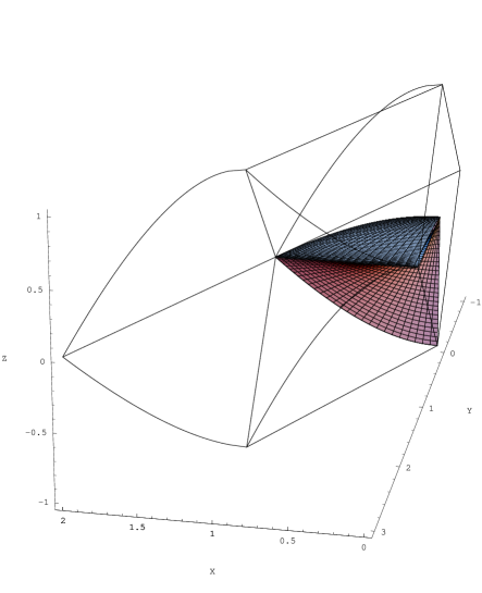
Figure 2: Graphical representation of the volumes occupied by $(X_{2},Y_{2},Z_{2})$ (transparent volume) and $(X_{1},Y_{1},Z_{1})$ (opaque volume). As expected the opaque volume is embedded into the transparent volume. This fact indicates that the amplitude damping channel cannot by simulated completely by the one-qubit environment.

The volume generated by $(X_{1},Y_{1},Z_{1})$ is plotted in Fig. 2 opaquelyaddress . As expected this volume is embedded in the lucid volume generated by $(X_{2},Y_{2},Z_{2})$. This means that the amplitude damping channel cannot be completely simulated by the one-qubit environment although it is in the arbitrary mixed-state as depolarizing channel. The volume for $(X_{1},Y_{1},Z_{1})$ can be computed analytically, which is $2/15$. Thus the volume ratio, i.e. opaque volume divided by transparent volume, is approximately $0.08$. This is much smaller than $3/8$, which is the volume ratio for the depolarizing channel.

V conclusion

We have studied the GAD channels simulated by the one-qubit mixed-state environment when the principal system is initially in the single-qubit pure state. Examing the affine map for the GAD channel simulated by two-qubit environment, we have found that $\xi=0$ with $\alpha=\gamma$, and $\alpha=\beta=\gamma$ are the GAD channel simulated by the one-qubit mixed-state environment. Representing the affine map as a three-dimensional volume, we have plotted the volume opaquely in Fig. 2. As expected, this volume is embedded in the total volume generated by the two-qubit environment. It turns out that the volume ratio is much smaller than $3/8$, which is the volume ratio for the depolarizing channel.

It seems to be interesting to explore the various different damping channels in this way. For example, let us consider the phase damping whose quantum operation is defined as $\varepsilon(\rho)=E_{0}\rho E_{0}^{\dagger}+E_{1}\rho E_{1}^{\dagger}$, where operation elements are

$$E_{0}=\left(\begin{array}[]{cc}1&0\\ 0&\sqrt{1-\lambda}\end{array}\right)\hskip 56.9055ptE_{1}=\left(\begin{array}[]{cc}0&0\\ 0&\sqrt{\lambda}\end{array}\right)$$ (101)

and $\lambda$ is a quantity related to a relaxation time. The affine map for the phase damping is thus $(r_{1},r_{2},r_{3})\rightarrow(r_{1}\sqrt{1-\lambda},r_{2}\sqrt{1-\lambda},r_{3})$. Therefore the effect of the phase damping is to shrink the Bloch sphere into ellipsoid. To explore the effect of one-qubit mixed-state environment in the phase damping process firstly we should generalize it by introducing four operation elements with keeping the general features of the standard phase damping. Next we should find same channels when the environment is single-qubit mixed states with making use of Eq.(34). It is unclear at least for us how to construct the generalized phase damping.

Another direction we would like to explore is to compute the entanglement measure when the environment is involved. Recently, the Groverian measure for mixed states was introduced in Ref.shapira06 Although it was shown in Ref.shapira06 that the Groverian measure for mixed states is entanglement monotone, the explicit computation of it for given mixed states is highly nontrivial mainly due to the maximization over purification while the analytic computation for the pure states is sometimes possibletama07-1 . Since environment in general makes the state of quantum system mixed state, it seems to be highly interesting to explore the role of entanglement in the damping process.

Acknowledgement: This work was supported by the Kyungnam University Research Fund, 2006.

References

- (1) R. P. Feynman, Int. J. Theor. Phys. 21 (1982) 467.
- (2) R. P. Feynman, Found. Phys. 16 (1986) 507.
- (3) P. W. Shor, Proc. 35th Annual Symposium on Foundations of Computer Science (1994) 124.
- (4) L. K. Grover, Proc. 28th Annual ACM Symposium on the Theory of Computing (1996) 212 [quant-ph/9605043].
- (5) L. K. Grover, Phys. Rev. Lett. 79 (1997) 325 [quant-ph/9706033].
- (6) C. Lavor, L. R. V. Manssur and R. Portugal, [quant-ph/0301079][quant-ph/0303175].
- (7) L. M. K. Vandersypen, M. Steffen, G. Breyta, C. S. Yannoni, M. H. Sherwood and I. L. Chuang, Nature 414 (2001) 883 [quant-ph/0112176].
- (8) C. Y. Lu, D. E. Browne, T. Yang and J. W. Pan, [arXiv:0705.1684].
- (9) P. G. Kwiat, J. R. Mitchell, P. D. D. Schwindt and A. G. White, J. Mod. Opt. 47 (20000) 257 [quant-ph/9905086].
- (10) P. Walther et al., Nature 434 (2005) 169 [quant-ph/0503126].
- (11) M. A. Nielsen and I. L. Chuang, Quantum Computation and Quantum Information (Cambridge Press, Cambridge, England, 2000).
- (12) B. Schumacher, Phys. Rev. A 54 (1996) 2614 [quant-ph/9604023].
- (13) S. Lloyd, Science 273 (1996) 1073.
- (14) B. M. Terhal, I. L. Chuang, D. P. DiVincenzo, M. Grassl and J. A. Smolin, Phys. Rev. A 60 (1999) 881 [quant-ph/9806095].
- (15) D. Bacon, A. M. Childs, I. L. Chuang, J. Kempe, D. Leung and X. Zhou, Phys. Rev. A 64 (2001) 062302 [quant-ph/0008070].
- (16) G. Narang and Arvind, Phys. Rev. A 75 (2007) 032305 [quant-ph/0611058].
- (17) B. Kraus and J. I. Cirac, Phys. Rev. A 63 (2001) 062309 [quant-ph/0011050].
- (18) The three-dimensional animation of the volumes and can be seen in http://rose.kyungnam.ac.kr/paper.htm.
- (19) D. Shapira, Y. Shimoni and O. Biham, Phys. Rev. A73 (2006) 044301 [quant-ph/0508108].
- (20) L. Tamaryan, D. K. Park and S. Tamaryan, arXiv0710.0571[quant-ph].