Kinetic ferromagnetism on a kagomé lattice

Abstract

We study strongly correlated electrons on a kagomé lattice at 1/6 (and 5/6) filling. They are described by an extended Hubbard Hamiltonian. We are concerned with the limit $|t|\ll V\ll U$ with hopping amplitude $t$, nearest-neighbor repulsion $V$ and on-site repulsion $U$. We derive an effective Hamiltonian and show, with the help of the Perron–Frobenius theorem, that the system is ferromagnetic at low temperatures. The robustness of ferromagnetism is discussed and extensions to other lattices are indicated.

Introduction.

Ferromagnetism in solids or molecules can be of different origin. The most common is spin exchange between electrons belonging to neighboring sites. Polarization of the spins and formation of a symmetric spin state reduces the effects of mutual Coulomb repulsions of the electrons due to the Pauli exclusion principle. The physics is the same as for intra-atomic Hund’s rule coupling, which also plays a significant role in the theory of ferromagnetism. The key ingredient of this mechanism is the potential energy of repulsive electron-electron interactions minimized by a symmetric spin state which is better at keeping electrons apart. This should be contrasted with the standard superexchange mechanism for antiferromagnetism where the kinetic energy of electrons is optimized instead. Hence it is often the competition between the potential and kinetic energies that determines the “winner”. This physics is illustrated, in its extreme limit, in the case of flat-band ferromagnetism Mielke (1991, 1992). Mielke pointed out that electrons in a half-filled flat band become fully spin-polarized for any strength of the on-site repulsion $U$. (One could also think of this effect as an extreme case of the Stoner instability in metals.)

Therefore it might appear surprising that ferromagnetism can also originate from purely kinetic effects. A prominent example is the ferromagnetic ground state (GS) discussed by Nagaoka Nagaoka (1966) which is due to the motion of a single hole in an otherwise half-filled Hubbard system. The argument based on the application of the Perron–Frobenius theorem shall be presented later. Although it is only valid in the limit of the infinite on-site Hubbard repulsion (to exclude the possibility of double occupancy) on a finite lattice, it demonstrates how ferromagnetism can result from the motion of the electrons or holes. The same theorem is also the basis of ferromagnetism due to three-particle ring exchange, a process first pointed out by Thouless Thouless (1965) in the context of ³He (following the original observation by Herring Herring (1962)) and later also studied in the context of Wigner glass Chakravarty et al. (1999) and frustrated magnets Misguich et al. (1999). In both cases, the ferromagnetic GS has the smoothest wavefunction and hence lowest kinetic energy.

Our introduction would not be complete without mentioning some other sources of ferromagnetism such as the RKKY interaction in metals or double-exchange (e.g., in manganites) to name a few. In this paper, however, we will be concerned with ferromagnetism of kinetic origin. In particular, we demonstrate that fermions on a partially filled kagomé lattice which are described by an extended one-band Hubbard model in the strong correlation limit have a ferromagnetic GS. (The difference with Mielke’s flat-band ferromagnetism is discussed later in the paper.) Again, the physics discussed here is motivated by the Perron–Frobenius theorem, but otherwise is quite different from Nagaoka’s and Thouless’ examples.

Model Hamiltonian.

We start from an extended one-band Hubbard model on a kagomé lattice with on-site repulsion $U$ and nearest-neighbor repulsion $V$. Using second quantized notation, the Hamiltonian is written as

$$H=-t\sum_{\langle i,j\rangle,\sigma}\left(c_{i\sigma}^{{\dagger}}c^{\vphantom{{\dagger}}}_{j\sigma}+\text{H.c.}\right)\\ +V\sum_{\langle i,j\rangle}n_{i}n_{j}+U\sum_{i}n_{i\uparrow}n_{i\downarrow}.$$ (1)

Here the operators $c^{\vphantom{{\dagger}}}_{i\sigma}$ ($c_{i\sigma}^{{\dagger}}$) annihilate (create) an electron with spin $\sigma$ on site $i$. The density operators are given by $n_{i}=n_{i\uparrow}+n_{i\downarrow}$ with $n_{i\sigma}=c_{i\sigma}^{{\dagger}}c^{\vphantom{{\dagger}}}_{i\sigma}$. The notation $\langle i,j\rangle$ refers to pairs of nearest neighbors.

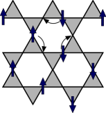
(a)	(b)
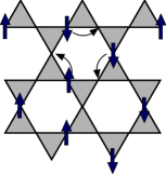
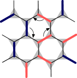
(c)	(d)
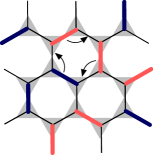
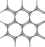
(e)	(f)

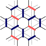
Figure 1: Panels (a) and (b) show two different configurations satisfying the constraint of zero or one electron per site and one electron of arbitrary spin per triangle. The arrows indicate possible ring-hopping processes. An equivalent colored dimer representation on a honeycomb lattice is shown in (c) and (d); the colors encode particle spins. Ring exchanges conserve the parity of the number of dimers on the sublattice shown in panel (e). Panel (f) shows the 24-site cluster used for the exact diagonalization. The dimers are arranged to maximize the next-nearest neighbor spin interaction along the dashed lines.

We first focus on the case of 1/6 filling (i.e., one electron per three sites). In the limit of strong correlations, when $|t|\ll V\ll U$ and $U\rightarrow\infty$, the possibility of doubly occupied sites is eliminated. First we assume that $t=0$. In that case the GS is macroscopically degenerate. All configurations with precisely one electron of arbitrary spin orientation on each triangle are GSs (see Figs. 1(a) and (b)). It is helpful to consider the honeycomb lattice which connects the centers of triangles of the kagomé lattice. Different GS configurations on the kagomé lattice correspond to different two-colored (spin) dimer configurations on the honeycomb lattice (particles are sitting here on links, see Fig. 1 (c) and (d)). They are orthogonal because any wavefunction overlap is neglected.

When $t\neq 0$, this GS degeneracy is lifted. In the lowest non-vanishing order in $t/V$, the effective Hamiltonian acting within the low-energy manifold spanned by the states with no double occupancy and exactly one electron per triangle becomes

$$H_{\text{hex}}=-g\sum_{\left\{\;\pspicture(0.0pt,2.84526pt)(5.69054pt,8.53581pt)\psset{linewidth=0.85358pt,linestyle=solid}{\psset{}\pspolygon(0.0pt,2.20508pt)(0.0pt,6.40186pt)(3.52814pt,8.53581pt)(7.25545pt,6.40186pt)(7.25545pt,2.20508pt)(3.52814pt,0.0pt)}\endpspicture\;\right\}\left\{\blacktriangle\blacksquare\bullet\right\}}\Big{(}\big{|}\;\pspicture(0.0pt,2.84526pt)(9.95845pt,17.07164pt)\psset{unit=21.33957pt}{\pspolygon(0.0pt,3.20093pt)(0.0pt,9.6028pt)(5.544pt,12.80374pt)(11.08803pt,9.6028pt)(11.08803pt,3.20093pt)(5.544pt,0.0pt)}\psset{linewidth=1.70715pt,linestyle=solid}{\psline(0.0pt,3.20093pt)(0.0pt,9.6028pt)}{\psline(5.544pt,12.80374pt)(11.08803pt,9.6028pt)}{\psline(11.08803pt,3.20093pt)(5.544pt,0.0pt)}{\psset{linecolor=gray,dotsize=4.26791pt 0.0}\psdots(0.0pt,6.40187pt)}{\psset{dotstyle=triangle*,linecolor=gray,dotsize=4.26791pt 0.0}\psdots(8.31602pt,11.20326pt)}{\psset{linecolor=gray,dotsize=4.26791pt 0.0,dotstyle=square*}\psdots(8.31602pt,1.60046pt)}\endpspicture\;\big{\rangle}\big{\langle}\;\pspicture(0.0pt,2.13396pt)(7.46884pt,12.80374pt)\psset{unit=21.33957pt}\psset{linewidth=0.64018pt,linestyle=solid}{\psset{}\pspolygon(0.0pt,3.20093pt)(0.0pt,9.6028pt)(5.544pt,12.80374pt)(11.08803pt,9.6028pt)(11.08803pt,3.20093pt)(5.544pt,0.0pt)}\psset{linewidth=1.70715pt,linestyle=solid}{\psline(5.544pt,12.80374pt)(0.0pt,9.6028pt)}{\psline(11.08803pt,3.20093pt)(11.08803pt,9.6028pt)}{\psline(5.544pt,0.0pt)(0.0pt,3.20093pt)}{\psset{linecolor=gray,dotsize=4.26791pt 0.0}\psdots(2.772pt,11.20326pt)}{\psset{dotstyle=triangle*,linecolor=gray,dotsize=4.26791pt 0.0}\psdots(11.20326pt,6.40187pt)}{\psset{linecolor=gray,dotsize=4.26791pt 0.0,dotstyle=square*}\psdots(2.772pt,1.60046pt)}\endpspicture\;\big{|}+\big{|}\;\pspicture(0.0pt,2.13396pt)(7.46884pt,12.80374pt)\psset{unit=21.33957pt}{\pspolygon(0.0pt,3.20093pt)(0.0pt,9.6028pt)(5.544pt,12.80374pt)(11.08803pt,9.6028pt)(11.08803pt,3.20093pt)(5.544pt,0.0pt)}\psset{linewidth=1.70715pt,linestyle=solid}{\psline(0.0pt,3.20093pt)(0.0pt,9.6028pt)}{\psline(5.544pt,12.80374pt)(11.08803pt,9.6028pt)}{\psline(11.08803pt,3.20093pt)(5.544pt,0.0pt)}{\psset{dotstyle=square*,linecolor=gray,dotsize=4.26791pt 0.0}\psdots(0.0pt,6.40187pt)}{\psset{linecolor=gray,dotsize=4.26791pt 0.0}\psdots(8.31602pt,11.20326pt)}{\psset{dotstyle=triangle*,linecolor=gray,dotsize=4.26791pt 0.0}\psdots(8.31602pt,1.60046pt)}\endpspicture\;\big{\rangle}\big{\langle}\;\pspicture(0.0pt,2.13396pt)(7.46884pt,12.80374pt)\psset{unit=21.33957pt}\psset{linewidth=0.64018pt,linestyle=solid}{\psset{}\pspolygon(0.0pt,3.20093pt)(0.0pt,9.6028pt)(5.544pt,12.80374pt)(11.08803pt,9.6028pt)(11.08803pt,3.20093pt)(5.544pt,0.0pt)}\psset{linewidth=1.70715pt,linestyle=solid}{\psline(5.544pt,12.80374pt)(0.0pt,9.6028pt)}{\psline(11.08803pt,3.20093pt)(11.08803pt,9.6028pt)}{\psline(5.544pt,0.0pt)(0.0pt,3.20093pt)}{\psset{linecolor=gray,dotsize=4.26791pt 0.0}\psdots(2.772pt,11.20326pt)}{\psset{dotstyle=triangle*,linecolor=gray,dotsize=4.26791pt 0.0}\psdots(11.20326pt,6.40187pt)}{\psset{linecolor=gray,dotsize=4.26791pt 0.0,dotstyle=square*}\psdots(2.772pt,1.60046pt)}\endpspicture\;\big{|}+\text{H.c.}\Big{)}$$ (2)

with $g=6t^{3}/V^{2}$. Here the Hamiltonian is written in terms of dimers on a honeycomb lattice and the sum is performed over all hexagons. The sum over the three symbols is taken over all possible color (spin) combinations of a flippable hexagon. Particles hop either clockwise or counter-clockwise around the hexagons. These processes can lead to different configurations, depending on the colors (spins) of the dimers. We observe that $H_{\text{hex}}$ does not cause a fermionic sign problem. In particular, the local constraint of having one fermionic dimer attached to each site allows for an enumeration of dimers such that only an even number of fermionic operators has to be exchanged when the matrix elements of $H_{\text{hex}}$ are calculated.

If one were to ignore the spin degrees of freedom (the colors of the dimers), the model would be equivalent to the quantum dimer model (QDM) studied in Ref. Moessner et al. (2001). Similarly to the QDM on a square lattice Rokhsar and Kivelson (1988), the effective Hamiltonian (2) conserves certain quantities – winding numbers – and connects configurations only when they belong to the same topological sector. (For the case of periodic boundary conditions, the winding numbers are defined by first orienting dimers so that the arrows point from the A to B sublattice, and second, by counting the net flow of these arrows across two independent essential cycles formed by the dual bonds.) The GS of the QDM was found to be three-fold degenerate in the thermodynamic limit, corresponding to the valence bond solid (VBS) plaquette phase with broken translational invariance. In what follows, we shall investigate the effects of quantum dynamics – the ring-exchange hopping of electrons (dimers) – on spin correlations. Note that $H_{\text{hex}}$ has no explicit spin dependency and conserves both $S^{z}_{\text{tot}}$ and the total spin $S_{\text{tot}}$.

Ferromagnetism from the Perron–Frobenius Theorem.

In short, the Perron–Frobenius theorem states that the largest eigenvalue of a symmetric $n\times n$ matrix with only positive elements is positive and non-degenerate, while the corresponding eigenvector is “nodeless”, i.e., can be chosen to have only positive components. (For a simple proof of this theorem, see e.g. Ninio (1976).) Applying this theorem to the (finite-dimensional) matrix $\exp{(-\tau\hat{H})}$ (for any $\tau>0$), one concludes that if all off-diagonal matrix elements of the Hamiltonian $\hat{H}$ are non-positive and the Hilbert space is connected by the quantum dynamics (meaning that any state can be reached from any other state by a repeated application of $\hat{H}$), then the GS is unique and nodeless. It is important to remember that the theorem only works for systems with a finite-dimensional Hilbert space.

To show the relation of this theorem to ferromagnetism, we now sketch the argument for Nagaoka’s ferromagnetism in the GS of an infinite $U$ Hubbard model (Eq. (1) with $V=0$, $U\to\infty$) with a single mobile hole (after Refs. Tasaki (1989); Tian (1990)). Denote a state with a single electron or hole on a site $i$ as $\left|i,\alpha\right\rangle$ where $\alpha=\left\{\sigma_{1},\ldots\sigma_{i-1},\sigma_{i+1},\ldots\sigma_{N}\right\}$ is the spin configuration of electrons. We use the convention $\left|i,\alpha\right\rangle=(-1)^{i}c_{1,\sigma_{1}}^{\dagger},\ldots c_{i-1,\sigma_{i-1}}^{\dagger}c_{i+1,\sigma_{i+1}}^{\dagger},\ldots c_{N,\sigma_{N}}^{\dagger}|0\rangle$. (No double occupancy is allowed if $U\to\infty$.) In this basis, the matrix elements of the hopping Hamiltonian are either $t$, for the states related by a single hop of the hole between two neighbor sites, or 0 otherwise. The Hamiltonian commutes with both $\hat{S}^{z}_{\text{tot}}$ and $\hat{S}^{2}_{\text{tot}}$. Our chosen basis consists of eigenstates of $\hat{S}^{z}_{\text{tot}}$ but not $\hat{S}^{2}_{\text{tot}}$, hence we can immediately separate the Hilbert space into sectors of fixed $S^{z}_{\text{tot}}$. Within each sector, the Hamiltonian matrix has exactly $z$ (the coordination number) nonzero entries in each row and each column. A direct inspection shows that a vector whose entries are all 1 is an eigenvector with the eigenvalue $zt$. If $t<0$ and tunneling of a single hole satisfies the connectivity condition, the Perron-Frobenius theorem applies and hence such a state is the GS (there can be no other state with positive coefficients only that is orthogonal to this one), which is unique for a finite system. (We remark that the sign of $t$ can always be changed on a bipartite lattice.) Clearly, this state is fully spin-polarized in the $S^{z}_{\text{tot}}=S_{\text{max}}=\pm N/2$ sectors, and since the Hamiltonian commutes with $\hat{S}^{2}_{\text{tot}}$, the state with ${S}^{2}_{\text{tot}}=(S_{\text{max}}+1)S_{\text{max}}$ must have the same energy in every $S^{z}_{\text{tot}}$ sector. But we already saw that the states with the energy $\mathcal{E}=zt$ are unique GSs in every sector, hence they must have the same ${S}^{2}_{\text{tot}}=(S_{\text{max}}+1)S_{\text{max}}$, QED. The obvious pitfalls may come from taking the thermodynamic limit or violating the connectivity condition: in both cases the nodeless, fully spin polarized state remain a GS but no claims can be made about other potential GSs.

Turning to our case, we remark that the sign of the plaquette flip in Eq. (2) can be always chosen negative, irrespective of the sign of the original tunneling amplitude $t$ – this is just a matter of a simple local gauge transformation Rokhsar and Kivelson (1988). Specifically, the sign of $g$ in Eq. (2) can be changed by multiplying all configurations $C$ with the color-independent factor $i^{\nu(C)}$ where $\nu(C)$ is the number of dimers on the sublattice shown in Fig. 1 (e). This fact might appear surprising though since the actual sign of $t$ can typically be gauged away only for the cases of bipartite or half-filled lattices. The reason the sign of $t$ turns out to be inconsequential in our case of the (non-bipartite) kagomé lattice away from half-filling is due to the constrained nature of the ring exchange quantum dynamics of Eq. (2). We therefore choose all off-diagonal matrix elements of $H_{\text{hex}}$ to be non-positive. This by itself is not yet sufficient to apply the Perron–Frobenius theorem since the quantum dynamics of dimers on a (bipartite) honeycomb lattice is explicitly non-ergodic: as we have mentioned earlier, the Hilbert space is broken into sectors corresponding to the winding numbers which are conserved under any local ring exchanges. On the other hand, the ring-exchange dynamics of dimers given by Eq. (2) is ergodic within each sector Saldanha and Tomei (1995). Therefore we consider each topological sector separately. The argument is very similar to the one presented earlier for Nagaoka’s ferromagnetism. For the $S^{z}_{\text{tot}}=S_{\text{max}}=\pm N_{\text{e}}/2$ spin sectors, the GS is unique, fully spin-polarized, and all elements of its eigenvector are positive.

For all other $S^{z}_{\text{tot}}$ sectors, however, the situation appears more complicated at first sight. The reason is a much bigger configuration space – essentially, we are now dealing with two-color dimer configurations. A given state can now be connected by a ring-exchange Hamiltonian to a larger number of states than it would if all dimers had the same color (spin). We formalize this by introducing the notion of descendant states $|C^{k}_{i}\rangle,\ k=1\dots 2^{N_{\text{e}}}$ – two-color dimer configurations obtained from the uncolored “parent” configuration $|C_{i}\rangle$ by simply coloring its dimers (i.e., assigning spins). The subspace of descendant states can be partitioned according the conserved $S^{z}_{\text{tot}}$. The resulting sectors, in general, have different dimensionality $D(S^{z}_{\text{tot}})$ equal to the number of distinct permutations of spins (colors). A crucial observation is that $\sum_{k}\langle C^{k}_{i}|H_{\text{hex}}|C^{m}_{j}\rangle=\langle C_{i}|H_{\text{hex}}|C_{j}\rangle$ for any $i$, $j$, $m$. The immediate consequence is that if $|\Psi_{0}\rangle\equiv|\Psi_{0}(N_{\text{e}}/2)\rangle=\sum_{i}\gamma_{i}|C_{i}\rangle$ is the GS in the $S^{z}_{\text{tot}}=S_{\text{max}}=\pm N_{\text{e}}/2$ spin sector, then $|\Psi_{0}(S^{z}_{\text{tot}})\rangle=D^{-1/2}(S^{z}_{\text{tot}})\sum_{i}\gamma_{i}\sum_{k}^{\prime}|C^{k}_{i}\rangle$ is an eigenstate with the same energy in any other $S^{z}_{\text{tot}}$ spin sector. (The sum over descendants $k$ is performed only within a given spin sector.) The SU(2) symmetry of the effective Hamiltonian (2) once again implies that $|\Psi_{0}(S^{z}_{\text{tot}})\rangle$ is a GS and is fully spin polarized.

Notice that the uniqueness of such a GS relies on the ergodicity of the Hamiltonian within each $S^{z}_{\text{tot}}$ spin sector. Numerical studies on finite clusters up to 48 kagomé lattice sites including different geometries show that this is in fact the case. Unfortunately, we were not able to provide a rigorous analytical argument. Should it turn not to be the case, it would open a possibility for degenerate GSs in $S^{z}_{\text{tot}}\neq S_{\text{max}}$ spin sectors. Still, at least one of the GSs is fully spin polarized Tasaki (1998).

While the Perron–Frobenius argument applies to finite systems, it does not withstand the thermodynamic limit. In particular, it is known that in the thermodynamic limit the ground state of the QDM is in the three-fold degenerate plaquette phase Moessner et al. (2001). We suspect that ferromagnetism survives this limit and coexists with such a broken symmetry state; a conclusive resolution of this point remains a subject of further research.

The ferromagnetic GS which we find here should not be mistaken with Mielke’s flat-band ferromagnetism Mielke (1991, 1992). In fact, Mielke has shown that a positive-$U$ Hubbard model with $V=0$ on a kagomé lattice at 5/6 filling has a fully spin-polarized GS. A detailed discussion of the differences to our case can be found below.

Stability of kinetic ferromagnetism.

In order to test the robustness of the ferromagnetic GS, we introduce by hand an additional next-nearest neighbor interaction, in the spirit of Didier Poilblanc, Karlo Penc, and Nic Shannon (2007):

$$H^{\prime}=H_{\text{hex}}+J\sum_{\langle\langle i,j\rangle\rangle}\left(S_{i}S_{j}-\frac{1}{4}n_{i}n_{j}\right).$$ (3)

By adding such a term, we attempt to frustrate the ferromagnetic state. Indeed, this term favors configurations such as the one shown in Fig. 1(f) which maximize the spin interactions by having electrons on the same sublattice. Not only the resulting charge order is expected to suppress the kinetic mechanism for ferromagnetism, the ferromagnetic order itself is now suppressed by antiferromagnetic fluctuations favored by the spin interactions for $J>0$.By gradually increasing $J/g$ towards strong antiferromagnetic coupling, we can estimate the stability of the ferromagnetic GS under the presence of short ranged perturbations.

Numerical Results.

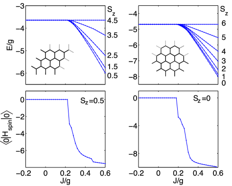
Figure 2: Exact diagonalization of the two-color dimer model on a 18-site (left panels) and 24-site (right panels) honeycomb cluster. The upper panels show the GS energies of different $S_{z}$ sectors as a function of next-nearest neighbor coupling $J/g$. The lower ones show the GS expectation values of the spin part of the Hamiltonian.

We calculate by means of exact diagonalization the GS of a two-color dimer model on a 18- and 24-site honeycomb lattice. The system corresponds to a 1/6 filled kagomé cluster with 27 and 36 sites, respectively. The calculations on the clusters of different size and geometry show qualitatively the same results.

The ground-state energies of the different $S_{z}$ sectors are degenerate as long as $J/g<J/g)_{c}\approx 0.2$, as shown in Fig. 2. This demonstrates the robustness of ferromagnetism induced by ring-hopping processes. Above the transition point $(J/g)_{c}\approx 0.2$ antiferromagnetic spin fluctuations are no longer suppressed. The ground-state degeneracy of the different $S_{z}$ sectors is lifted and the true GS is the one with the lowest $|S_{z}|$. The gain in kinetic energy decreases correspondingly since the spin fluctuations cause nodes in the wavefunction. The expectation value of $H_{\text{spin}}$ shows a jump at $(J/g)_{c}$ (see Fig.  2). Note that a small second jump at $J/g\approx 0.45$ found for the 18 site cluster is an effect of geometry. The observed findings demonstrate a considerable robustness of ferromagnetism generated by kinetic processes. In the limit $J/g\rightarrow\infty$, the kinetic processes are unimportant and the GS is that of a Heisenberg antiferromagnet on a kagomé lattice. One of the configurations which maximize the spin interactions is shown in Fig. 1 (f).

The above considerations can also be applied to the case of 5/6 filling due to the arbitrary choice of sign of $g$ in Eq. (2). In addition, a ferromagnetic GS is found numerically for a filling factor of 1/3. With two occupied sites per triangle, we obtain a fully packed loop covering of the honeycomb lattice instead of a dimer covering. As before, there is no sign problem in the strong coupling limit. However, the effective Hamiltonian is not ergodic in the 1/3 filled case and thus the Perron–Frobenius theorem does not rule out other GSs which are not fully spin polarized. Numerical studies confirm a ferromagnetic GS which is much less robust – antiferromagnetic fluctuations occur already at very small ratios $(J/g)$. A more detailed discussion is left to an extended version of this paper.

We conclude by reiterating the difference between the two mechanisms for ferromagnetism in a Hubbard model on the kagomé lattice: the one presented here and the flat-band mechanism discussed in Refs. Mielke (1991, 1992); Tasaki (1998). The flat-band ferromagnetism was demonstrated for the case of $V=0$ in the Hamiltonian (1), while our mechanism requires $V\to\infty$. In Mielke’s case, ferromagnetism has been predicted for the range of fillings between $5/6$ and $11/12$ and any value of $U>0$. The connection between the sign of the tunneling amplitude $t$ and the electron concentration is crucial. This is because the tight binding model on a kagomé lattice has one of its three bands completely flat: the lowest band for the case of $t<0$ or the highest band for the case of $t>0$. On the other hand, the mechanism presented here is insensitive to the sign of $t$ and, as we have already mentioned in the introduction, is of kinetic rather than of potential origin. Furthermore, Perron–Frobenius theorem is not applicable in Mielke’s case Tasaki (1998), instead the proof was based on graph-theoretical methods. By contrast, the kinetic ferromagnetism studied in this letter relies crucially on strong electron–electron repulsion $U\gg V\to\infty$; hence it belongs to a different class from flat-band ferromagnetism. Despite certain similarities, it must also be distinguished from Thouless’ three-particle ring exchange mechanism: the crucial difference is that a standard three-particle ring exchange leaves the particles at the original locations, it simply cyclically permutes them. In our case the particles actually move; the initial and final configurations are distinct.

Thus the mechanism found in this letter represents a new generic type of kinetic ferromagnetism. An interesting question is to what extent the ferromagnetism of the form found here can be extended to other lattice structures. A particularly interesting case is the pyrochlore lattice. For the strong correlation limit at $1/8$ filling one can use the Perron–Frobenius-based argument as well, implying a ferromagnetic GS. Again, this and other cases will be discussed in the extended version of this paper.

The authors would like to thank G. Misguich and R. Kenyon for illuminating and helpful discussions.

References

- Mielke (1991) A. Mielke, J. Phys. A: Math. Gen. 24, L73 (1991).
- Mielke (1992) A. Mielke, J. Phys. A: Math. Gen. 25, 4335 (1992).
- Nagaoka (1966) Y. Nagaoka, Phys. Rev. 147, 392 (1966).
- Thouless (1965) D. J. Thouless, Proc. Phys. Soc. 86, 893 (1965).
- Herring (1962) C. Herring, Rev. Mod. Phys. 34, 631 (1962).
- Chakravarty et al. (1999) S. Chakravarty, S. Kivelson, C. Nayak, and K. Voelker, Phil. Mag. B 79, 859 (1999), eprint cond-mat/9805383.
- Misguich et al. (1999) G. Misguich, C. Lhuillier, B. Bernu, and C. Waldtmann, Phys. Rev. B 60, 1064 (1999).
- Moessner et al. (2001) R. Moessner, S. L. Sondhi, and P. Chandra, Phys. Rev. B 64, 144416 (2001), eprint cond-mat/0106288.
- Rokhsar and Kivelson (1988) D. S. Rokhsar and S. A. Kivelson, Phys. Rev. Lett. 61, 2376 (1988).
- Ninio (1976) F. Ninio, J. Phys. A: Math. Gen. 9, 1281 (1976); 10, 1259 (1977).
- Tasaki (1989) H. Tasaki, Phys. Rev. B 40, 9192 (1989).
- Tian (1990) G.-S. Tian, J. Phys. A: Math. Gen. 23, 2231 (1990).
- Saldanha and Tomei (1995) N. Saldanha and C. Tomei, Resenhas 2, 239 (1995).
- Tasaki (1998) H. Tasaki, Prog. Theor. Phys. 99, 489 (1998), eprint cond-mat/9712219.
- Didier Poilblanc, Karlo Penc, and Nic Shannon (2007) D. Poilblanc, K. Penc, and N. Shannon, unpublished (2007), eprint cond-mat/0209423.