Quark Loop Contributions to Neutron, Deuteron, and Mercury EDMs from Supersymmetry without R parity

Abstract

We present a detailed analysis together with numerical calculations on one-loop contributions to the neutron, deuteron and mercury electric dipole moment from supersymmetry without R parity, focusing on the quark-scalar loop contributions. Being proportional to top Yukawa and top mass, such contributions are often large, and since these are proportional to hitherto unconstrained combinations of bilinear and trilinear RPV parameters, they are all the more interesting. Complete formulas are given for the various contributions through the quark dipole operators including the contribution from color dipole operator. The contribution from color dipole operator is found to be similar order in magnitude when compared to the electric dipole operator and should be included in any consistent analysis. Analytical expressions illustrating the explicit role of the R-parity violating parameters are given following perturbative diagonalization of mass-squared matrices for the scalars. Dominant contributions come from the combinations $B_{i}^{\ast}\lambda^{\prime}_{ij1}$ for which we obtain robust bounds. It turns out that neutron and deuteron EDMs receive much stronger contributions than mercury EDM and any null result at the future deuteron EDM experiment or Los Alamos neutron EDM experiment can lead to extra-ordinary constraints on RPV parameter space. Even if R-parity violating couplings are real, CKM phase does induce RPV contribution and for some cases such a contribution is as strong as contribution from phases in the R-parity violating couplings. Hence, we have bounds directly on $|B_{i}^{\ast}\lambda^{\prime}_{ij1}|$ even if the RPV parameters are all real. Interestingly, even if slepton mass and/or $\mu_{\scriptscriptstyle 0}$ is as high as 1 TeV, it still leads to neutron EDM that is an order of magnitude larger than the sensitivity at Los Alamos experiment. Since the results are not much sensitive to $\tan\beta$, our constraints will survive even if other observables tighten the constraints on $\tan\beta$.

I Introduction

The problems of neutrino mass, baryogenesis, dark matter, dark energy and gauge hierarchy, provide unambiguous hints toward physics beyond standard model (SM). Whereas a direct discovery of new physics particles at colliders is indispensable, a search for alternative observables could not only provide a means to discovery of new physics but also prove complimentary by hinting at favorable regions in parameter space. Discrete symmetries and their violations have been crucial to establishing and validating the SM. Forty years after the discovery of CP-violation cpv , its experimentally observed effects in the K and B-meson systems cpv ; KBcpv are generally compatible with the standard model (SM) predictions with the Kobayashi-Maskawa (KM) phase as its sole source. The search for more CP violating observables is keenly pursued at ongoing and upcoming B physics experiments, and it is largely confined to flavor changing sector. Within the flavor diagonal sector, P and T violating electric dipole moments (EDMs) of fermions Landaucpv , heavy atoms and molecules are interesting CP violating observables that provide essentially background free and sensitive probes of physics beyond SM pospelov-review ; ginges-review . Though the search for non-vanishing EDM has so far yielded null results, the present experimental scenario with regard to EDM measurements is very encouraging, with most of them well within the range of interesting predictions from physics beyond SM. For the convenience of reader, below we briefly describe the current status of EDM experiments. This will also serve to motivate our case for specific new physics contributions that we discuss here.

Since the early work of Purcell and Ramsey purcell , EDM experiments have dramatically improved in precision. The standard method for measuring a permanent EDM of a particle is by placing it in an external electric field $E$ and looking for a shift in energy that is linear in $E$. This explains the focus on the electrically neutral candidates for EDM measurements. Naively, the Schiff screening theorem prevents any measurement of atomic EDM. Indeed, the assumptions of Schiff theorem, namely the point-sized nucleus and non-relativistic limit, are significantly violated in heavy atoms and hence facilitate EDM measurement. Ironically, the shielding which is complete in non-relativistic limit, actually produces an enhancement in the realistic relativistic limit salpeter-58 . Sanders sanders-65 pointed out that due to relativistic magnetic effects, the atomic EDM induced in heavy atoms can be strongly enhanced compared to electron EDM inducing it, leading to the best limit on electron EDM. The enhancement factor can be over two orders of magnitude. For the case of paramagnetic atoms, the best bound so far is for the thallium ($~{}^{205}\mathrm{Tl}$), $|d_{\mathrm{Tl}}|<9.0\times 10^{-25}$ (90%C.L.) leading to the tightest limit on electron EDM $|d_{e}|\leq 1.6\times 10^{-27}$ Tl-bound . Note that the numbers are in the standard $e$ cm unit, which is assumed throughout the paper. For the case of diamagnetic atoms, mercury ($~{}^{199}\mathrm{Hg}$) EDM is best constrained by the Washington group, the bound being, $|d_{\mathrm{Hg}}|<2\times 10^{-28}$ (95 % C.L.) Hg-bound . An upgraded experiment is expected to improve the accuracy by a factor of four Hg-upgrade . The violation of Schiff theorem comes about due to the finite size effect of the nucleus. For the nucleon EDM, the best bound so far is on the neutron EDM from the Grenoble experiment, $|d_{n}|<6.3\times 10^{-26}$ (90% C.L.) expNEDM . The most recent result from the same experiment is $|d_{n}|<3\times 10^{-26}$ nEDM-recent . It is expected to reach a goal of $|d_{n}|<1.5\times 10^{-26}$ nEDM-goal . The Los Alamos neutron EDM experiment will provide two orders of magnitude improvement, probing $d_{n}$ down to order $10^{-28}$ nEDM-SNS . The standard method of measuring the energy shift linear in electric field fails for the EDM of charged particle due to acceleration of charged particle. However, in recent years a new dedicated method of searching for EDM of charged particles in storage rings has been developed farley-PRL ; semer-00 . A muon EDM experiment is proposed that is expected to reach a sensitivity of $10^{-24}$ which is an improvement of a factor of $10^{5}$ to $10^{6}$ over the last CERN muon g-2 experiment jpark-letter . A deuteron EDM experiment, again using storage ring is proposed, that would reach a sensitivity of $10^{-27}$ that is 10 to 100 times better than current EDM limits in terms of sensitivity to quark EDM and QCD $\theta$ parameter dt-edm-proposal .

With so many exciting ongoing and upcoming experiments, EDM searches certainly provide complementary alternative to probe physics beyond the SM. In this work we will focus on the neutron, deuteron and mercury EDM. As an example of physics beyond SM, we shall focus on supersymmetry (SUSY) without R-parity or the generic supersymmetric standard model GSSM . When the large number of baryon or lepton number violating terms are removed by imposing an ad hoc discrete symmetry called R-parity, one obtains the MSSM Lagrangian. GSSM is a complete theory of SUSY without R-parity, where all kinds of R-parity violating (RPV) terms are admitted without bias. It is generally better motivated than ad hoc versions of RPV theories. The MSSM itself, without extension such as adding SM singlet superfields and admitting violation of lepton number, cannot accommodate neutrino mass mixings and hence oscillations neutrino . Given SUSY, the GSSM is actually conceptually the simplest framework to accommodate the latter. The large number of a priori arbitrary RPV terms do make phenomenology complicated. However, the origin of the (pattern of) values for the couplings may be considered to be on the same footing as that of the SM Yukawa couplings. For example, it has been shown in u1 that one can understand the origin, pattern and magnitude of all the RPV terms as a result of a spontaneously broken anomalous Abelian family symmetry model.

As we will see in the next section, EDM of mercury, deuteron and neutron are expressible in terms of quark EDM and color EDM (CEDM). Neutron EDM is an old favorite and within SM, the CKM phase contribution starts at three loop level shabalin . Generic (R-parity conserving) SUSY contributions starts at one loop level and hence can be large arnowitt-D90 ; oshimo-D92 ; nath-D98 ; oshimo-D97 ; dp-D01 ; olive-B98 ; hisano-D04 ; pospelov-ritz-D01 ; farzan-J05 ; luca-05 ; farzan-06 . Most of the phenomenology studies of the case admitting R-parity violation have largely been confined to the trilinear superpotential parameters. Within the latter framework, it has been shown that contributions to fermion EDMs start at two loop level 2loop . Striking one-loop contributions are, however, identified and discussed based on the GSSM framework nedm ; chun . Under that generic setting, all RPV couplings are considered without bias. Note that studies of RPV physics under such a generic setting is uncommon. Not only that a priori approximations were usually taken on the form of R-parity violation especially on the set of bilinear parameters, such approximations were often times not clearly stated, if appreciated well enough. They may be confused with the flavor basis choice issues (see Ref.GSSM for detailed discussions on the aspects). EDM study from Godbole el.al in Ref.2loop , however, did state explicitly the bilinear couplings were neglected in their study. The one loop contributions are exactly resulted from combinations of a bilinear and a trilinear RPV couplings. Similarly, flavor off-diagonal dipole moment contributing to the case of the $b\rightarrow s\gamma$ decay bsg and that of the $\mu\rightarrow e\gamma$ mueg decay at one-loop level have also been presented. That is the approach taken here. In Ref.nedm , the one loop EDM contributions from the gluino loop, chargino-like loop, neutralino-like loop are studied numerically in some details. It shows that the RPV parameter combination $\mu_{i}^{*}\lambda^{\!\prime}_{i\scriptscriptstyle 1\!1}$ dominates. with small sensitivity to the value of $\tan\!\beta$. The experimental bound on neutron EDM is used to constrain the model parameter space, especially the RPV part. However, the alternative one-loop contribution containing a quark and a scalar in the loop is also important. For the case of down quark EDM, it contains a top-quark loop and hence proportional to top mass and top Yukawa, thus can giving rise to very large contribution. We give complete 1-loop formulas for these contributions to the EDMs of the up- and down-sector quarks, with full incorporation of family mixings (in Ref.nedm , family mixing was neglected for simplicity). We present numerical analysis of quark-scalar loop contributions from all possible combinations of RPV parameters. Besides the familiar $\mu_{i}^{*}\lambda^{\!\prime}_{i\scriptscriptstyle 1\!1}$, there are a list of combinations of the type $B_{i}^{*}\lambda^{\!\prime}_{ijk}$ which are particularly interesting and will be the focus of this paper. In comparison to the earlier works nedm ; chun , our investigation provides more extensive results, both analytically as well as numerically with elaboration on some physics issues as well as includes contributions to deuteron and mercury EDM. We obtain bounds on combinations of RPV couplings which are otherwise unavailable. In fact, as we will see, any null results of future EDM experiments lead to stringent constraints on RPV parameters that have not been constrained so far.

Note that we decouple any explicit discussion of leptonic EDM, like for the electron and muon as well as $d_{\mathrm{Tl}}$ in which the electron EDM has a dominant role, from the study here. Unlike the case of the R-parity conserving contributions, the RPV contributions to EDMs of the quark and lepton sectors have quite independent origin. For the lepton sector, it involves the $\lambda$-couplings, rather than the $\lambda^{\!\prime}$-couplings. Hence, a whole set of different combinations of RPV parameters are to be constrained by the leptonic EDMs numbers — not to be addressed in this paper.

The structure of the paper is as follows. In the next section we describe our notation and framework, the so called single-VEV parametrization (SVP). We will also describe the formula for neutron, deuteron and mercury EDM in terms of quark EDM and chromoelectric dipole moment (CEDM). In section III, we will describe the quark loop contribution to quark EDM and CEDM coming from a combination of a bilinear and trilinear RPV couplings. In section IV we will discuss the results and in section V we will conclude.

II Formulation and Notation

We summarize the model here while setting the notation. Details of the formulation adopted is elaborated in Ref.GSSM . The most general renormalizable superpotential for the supersymmetric SM (without R-parity) can be written as

$$W\!\! = \!\varepsilon_{ab}\Big{[}\mu_{\alpha}\hat{H}_{u}^{a}\hat{L}_{\alpha}^{b}+h_{ik}^{u}\hat{Q}_{i}^{a}\hat{H}_{u}^{b}\hat{U}_{k}^{\scriptscriptstyle C}+\lambda_{\alpha jk}^{\!\prime}\hat{L}_{\alpha}^{a}\hat{Q}_{j}^{b}\hat{D}_{k}^{\scriptscriptstyle C}$$ (1)

$$+ \frac{1}{2}\,\lambda_{\alpha\beta k}\hat{L}_{\alpha}^{a}\hat{L}_{\beta}^{b}\hat{E}_{k}^{\scriptscriptstyle C}\Big{]}+\frac{1}{2}\,\lambda_{ijk}^{\!\prime\prime}\hat{U}_{i}^{\scriptscriptstyle C}\hat{D}_{j}^{\scriptscriptstyle C}\hat{D}_{k}^{\scriptscriptstyle C}\;,$$

where $(a,b)$ are $SU(2)$ indices, $(i,j,k)$ are the usual family (flavor) indices, and $(\alpha,\beta)$ are extended flavor index going from $0$ to $3$. In the limit where $\lambda_{ijk},\lambda^{\!\prime}_{ijk},\lambda^{\!\prime\prime}_{ijk}$ and $\mu_{i}$ all vanish, one recovers the expression for the R-parity preserving case, with $\hat{L}_{0}$ identified as $\hat{H}_{d}$. Without R-parity imposed, the latter is not a priori distinguishable from the $\hat{L}_{i}$’s. Note that $\lambda$ is antisymmetric in the first two indices, as required by the $SU(2)$ product rules, as shown explicitly here with $\varepsilon_{\scriptscriptstyle 12}=-\varepsilon_{\scriptscriptstyle 21}=1$. Similarly, $\lambda^{\!\prime\prime}$ is antisymmetric in the last two indices, from $SU(3)_{\scriptscriptstyle C}$.

The large number of new parameters involved, however, makes the theory difficult to analyze. An optimal parametrization, called the single-VEV parametrization (SVP) has been advocatedru2 to make the the task manageable. Here, the choice of an optimal parametrization mainly concerns the 4 $\hat{L}_{\alpha}$ flavors. Under the SVP, flavor bases are chosen such that : 1) among the $\hat{L}_{\alpha}$’s, only $\hat{L}_{0}$, bears a VEV, i.e. $\langle\hat{L}_{i}\rangle\equiv 0$; 2) $h^{e}_{jk}(\equiv\lambda_{0jk})=\frac{\sqrt{2}}{v_{\scriptscriptstyle 0}}\,{\rm diag}\{m_{\scriptscriptstyle 1},m_{\scriptscriptstyle 2},m_{\scriptscriptstyle 3}\}$; 3) $h^{d}_{jk}(\equiv\lambda^{\!\prime}_{0jk}=-\lambda_{j0k})=\frac{\sqrt{2}}{v_{\scriptscriptstyle 0}}{\rm diag}\{m_{d},m_{s},m_{b}\}$; 4) $h^{u}_{ik}=\frac{\sqrt{2}}{v_{\scriptscriptstyle u}}V_{\!\mbox{\tiny CKM}}^{\!\scriptscriptstyle T}\;{\rm diag}\{m_{u},m_{c},m_{t}\}$, where ${v_{\scriptscriptstyle 0}}\equiv\sqrt{2}\,\langle\hat{L}_{0}\rangle$ and ${v_{\scriptscriptstyle u}}\equiv\sqrt{2}\,\langle\hat{H}_{u}\rangle$. The big advantage of here is that the (tree-level) mass matrices for all the fermions do not involve any of the trilinear RPV couplings, though the approach makes no assumption on any RPV coupling including even those from soft SUSY breaking; and all the parameters used are uniquely defined, with the exception of some possibly removable phases.

The soft SUSY breaking part of the Lagrangian in GSSM can be written as follows :

$$V_{\rm soft} = \epsilon_{\!\scriptscriptstyle ab}B_{\alpha}\,H_{u}^{a}\tilde{L}_{\alpha}^{b}+\epsilon_{\!\scriptscriptstyle ab}\left[\,A^{\!\scriptscriptstyle U}_{ij}\,\tilde{Q}^{a}_{i}H_{u}^{b}\tilde{U}^{\scriptscriptstyle C}_{j}+A^{\!\scriptscriptstyle D}_{ij}H_{d}^{a}\tilde{Q}^{b}_{i}\tilde{D}^{\scriptscriptstyle C}_{j}+A^{\!\scriptscriptstyle E}_{ij}H_{d}^{a}\tilde{L}^{b}_{i}\tilde{E}^{\scriptscriptstyle C}_{j}\,\right]+{\rm h.c.}$$ (2)

$$+ \epsilon_{\!\scriptscriptstyle ab}\left[\,A^{\!\scriptscriptstyle\lambda^{\prime}}_{ijk}\tilde{L}_{i}^{a}\tilde{Q}^{b}_{j}\tilde{D}^{\scriptscriptstyle C}_{k}+\frac{1}{2}\,A^{\!\scriptscriptstyle\lambda}_{ijk}\tilde{L}_{i}^{a}\tilde{L}^{b}_{j}\tilde{E}^{\scriptscriptstyle C}_{k}\right]+\frac{1}{2}\,A^{\!\scriptscriptstyle\lambda^{\prime\prime}}_{ijk}\tilde{U}^{\scriptscriptstyle C}_{i}\tilde{D}^{\scriptscriptstyle C}_{j}\tilde{D}^{\scriptscriptstyle C}_{k}+{\rm h.c.}$$

$$+ \tilde{Q}^{\dagger}\tilde{m}_{\!\scriptscriptstyle{Q}}^{2}\,\tilde{Q}+\tilde{U}^{\dagger}\tilde{m}_{\!\scriptscriptstyle{U}}^{2}\,\tilde{U}+\tilde{D}^{\dagger}\tilde{m}_{\!\scriptscriptstyle{D}}^{2}\,\tilde{D}+\tilde{L}^{\dagger}\tilde{m}_{\!\scriptscriptstyle{L}}^{2}\tilde{L}+\tilde{E}^{\dagger}\tilde{m}_{\!\scriptscriptstyle{E}}^{2}\,\tilde{E}+\tilde{m}_{\!\scriptscriptstyle H_{\!\scriptscriptstyle u}}^{2}\,|H_{u}|^{2}$$

$$+\frac{M_{\!\scriptscriptstyle 1}}{2}\tilde{B}\tilde{B}+\frac{M_{\!\scriptscriptstyle 2}}{2}\tilde{W}\tilde{W}+\frac{M_{\!\scriptscriptstyle 3}}{2}\tilde{g}\tilde{g}+{\rm h.c.}\;,$$

where we have separated the R-parity conserving ones from the RPV ones ($H_{d}\equiv\hat{L}_{0}$) for the $A$-terms. Note that $\tilde{L}^{\dagger}\tilde{m}_{\!\scriptscriptstyle\tilde{L}}^{2}\tilde{L}$, unlike the other soft mass terms, is given by a $4\times 4$ matrix. Explicitly, $\tilde{m}_{\!\scriptscriptstyle{L}_{00}}^{2}$ is $\tilde{m}_{\!\scriptscriptstyle H_{\!\scriptscriptstyle d}}^{2}$ of the MSSM case while $\tilde{m}_{\!\scriptscriptstyle{L}_{0k}}^{2}$’s give RPV mass mixings.

Details of the tree-level mass matrices for all fermions and scalars are summarized in Ref.GSSM . For the analytical appreciation of many of the results, approximate expressions of all the RPV mass mixings are very useful. The expressions are available from perturbative diagonalization of the mass matricesGSSM .

III The Quark Loop Contribution to neutron, deuteron and Mercury EDM

As we will see toward the end of this section, neutron, deuteron, and mercury EDMs are ultimately expressible in terms of quark EDMs and CEDMs. Quark EDMs and CEDMs are typically defined from the following effective Lagrangian:

$${\cal L}_{\mathrm{eff.}}=-\frac{i}{2}d^{\!\scriptscriptstyle E}_{f}\bar{f}\sigma_{\mu\nu}\gamma_{5}fF^{\mu\nu}-\frac{i}{2}d^{\!\scriptscriptstyle C}_{f}\bar{f}\sigma_{\mu\nu}\gamma_{5}T^{a}fG^{\mu\nu a}\;.$$ (3)

Here, $d^{\!\scriptscriptstyle E}_{f}$ and $d^{\!\scriptscriptstyle C}_{f}$ are EDM and CEDM, respectively, of a quark flavor $f$. We perform calculations of the one-loop EDM diagrams using mass eigenstates with their effective couplings. The approach frees our numerical results from the mass-insertion approximation more commonly adopted in the type of calculations, while analytical discussions based of the perturbative diagonalization formulae help to trace the major role of the RPV couplings, especially those of the bilinear type. The interesting class of one-loop contributions are obtained from diagrams involving a bilinear-trilinear parameter combinations, which were seldom studied by most other authors on RPV physics. The bilinear parameters come into play through mass mixings induced among the fermions and scalars (slepton and Higgs states), while the trilinear parameter enters a effective coupling vertex. The basic features are the same as those reported in the studies of the various related processesnedm ; bsg . Among the latter, our recently available reports on $b\rightarrow s+\gamma$ bsg are particularly noteworthy, for comparison. The $d$ quark dipole plays a more important role over that of the $u$ quark, when RPV contributions are involved. The $b\rightarrow s+\gamma$ diagram is, of course, nothing other than a flavor off-diagonal version of a down-sector quark dipole moment diagram.

Unlike the SM Yukawa couplings, the RPV Yukawa couplings are mostly not so strongly constrained in magnitudes bounds , and are sources of flavor mixings. A trilinear $\lambda_{\alpha jk}^{\!\prime}$ coupling couples a quark to another one, of the same or different charge, and a generic scalar, neutral or charged accordingly. The coupling together with a SM Yukawa coupling at another vertex contributes to the EDMs through some scalar mass eigenstates with RPV mass mixings involved, as illustrated in Fig. 1. As the SM Yukawas are flavor diagonal, the charged scalar loops contribute by invoking CKM mixings. Note that under the SVP adopted, the $\lambda_{\alpha jk}^{\!\prime}$ parameters have quark flavor indices actually defined in the $d$-sector quark mass eigenstate basis. Analytically, we have the formula for the electric dipole form factor for quark flavor $f$,

$$\small\left({\frac{d^{\!\scriptscriptstyle E}_{\scriptscriptstyle f}}{e}}\right)_{\!\!\phi^{\mbox{-}}}=-{\frac{\alpha_{\!\mbox{\tiny em}}}{4\pi\,\sin\!^{2}\theta_{\!\scriptscriptstyle W}}}\;\sum_{m}^{\prime}\sum_{n=1}^{3}\,\mbox{Im}(\widetilde{\cal C}_{\scriptscriptstyle nmi}^{\scriptscriptstyle\!L}\widetilde{\cal C}^{\scriptscriptstyle\!R\ast}_{\scriptscriptstyle nmi})\frac{{M}_{\!\scriptscriptstyle f_{n}^{\prime}}}{M_{\!\scriptscriptstyle\tilde{\ell}_{m}}^{2}}\;\left[({\cal Q}_{\!f}-{\cal Q}_{\!f^{\prime}})\;F_{4}\!\left({\frac{{M}_{\!\scriptscriptstyle f_{n}^{\prime}}^{2}}{M_{\!\scriptscriptstyle\tilde{\ell}_{m}}^{2}}}\right)-{\cal Q}_{\!f^{\prime}}\;F_{3}\!\left({\frac{{M}_{\!\scriptscriptstyle f_{n}^{\prime}}^{2}}{M_{\!\scriptscriptstyle\tilde{\ell}_{m}}^{2}}}\right)\right]\;,$$ (4)

and for the chromo-electric dipole form factor,

$$\left(d^{\!\scriptscriptstyle C}_{\scriptscriptstyle f}\right)_{\!\!\phi^{\mbox{-}}}={\frac{g_{s}\alpha_{\!\mbox{\tiny em}}}{4\pi\,\sin\!^{2}\theta_{\!\scriptscriptstyle W}}}\;\sum_{m}^{\prime}\sum_{n=1}^{3}\,\mbox{Im}(\widetilde{\cal C}_{\scriptscriptstyle nmi}^{\scriptscriptstyle\!L}\widetilde{\cal C}^{\scriptscriptstyle\!R\ast}_{\scriptscriptstyle nmi})\frac{{M}_{\!\scriptscriptstyle f_{n}^{\prime}}}{M_{\!\scriptscriptstyle\tilde{\ell}_{m}}^{2}}\;{\cal Q}_{\!f^{\prime}}\;F_{3}\!\left({\frac{{M}_{\!\scriptscriptstyle f_{n}^{\prime}}^{2}}{M_{\!\scriptscriptstyle\tilde{\ell}_{m}}^{2}}}\right)\;.$$ (5)

Here, $F_{3}(x)$ and $F_{4}(x)$ are Inami-Lim loop functions, given as:

$$F_{3}(x) = \frac{1}{2(1-x)^{3}}\,(-3+4\,x-x^{2}-2\,\ln x)\;,$$ (6)

$$F_{4}(x) = \frac{1}{2(1-x)^{3}}\,(1-x^{2}+2\,x\,\ln x)\;.$$ (7)

For $f=u$ ($i=1$), the coefficients $\widetilde{\cal C}_{\scriptscriptstyle nmi}^{\!\scriptscriptstyle L,\scriptscriptstyle R}$ are defined by the interaction Lagrangian,

$${\cal L}^{u}={g_{\scriptscriptstyle 2}}\overline{\Psi}(d_{n})\Phi^{\dagger}(\phi_{m}^{{\mbox{-}}})\left[\widetilde{\cal C}^{\!\scriptscriptstyle L}_{\scriptscriptstyle nmi}{1-\gamma_{\scriptscriptstyle 5}\over 2}+\widetilde{\cal C}^{\!\scriptscriptstyle R}_{\scriptscriptstyle nmi}{1+\gamma_{\scriptscriptstyle 5}\over 2}\right]{\Psi}({u_{i}})\ +\mbox{h.c.}\;,$$ (8)

$$\widetilde{\cal C}_{\scriptscriptstyle nmi}^{\scriptscriptstyle L\ast} = \frac{y_{d_{n}}}{g_{\scriptscriptstyle 2}}\,V_{\!\mbox{\tiny CKM}}^{in}{\cal D}_{2m}^{l^{\ast}}+\frac{\lambda_{jkn}^{\!\prime\ast}}{g_{\scriptscriptstyle 2}}\,V_{\!\mbox{\tiny CKM}}^{ik}{\cal D}_{(j+2)m}^{l^{\ast}}\;,$$

$$\widetilde{\cal C}_{\scriptscriptstyle nmi}^{\scriptscriptstyle R\ast} = \frac{y_{u_{i}}}{g_{\scriptscriptstyle 2}}V_{\!\mbox{\tiny CKM}}^{in}\,{\cal D}_{1m}^{l^{\ast}}\;,$$ (9)

and, for $f=d$ ($i=1$), the coefficients $\widetilde{\cal C}_{\scriptscriptstyle nmi}^{\!\scriptscriptstyle L,\scriptscriptstyle R}$ are defined by the interaction Lagrangian,

$${\cal L}^{d}={g_{\scriptscriptstyle 2}}\overline{\Psi}(u_{n})\Phi(\phi_{m}^{{\mbox{-}}})\left[\widetilde{\cal C}^{\!\scriptscriptstyle L}_{\scriptscriptstyle nmi}{1-\gamma_{\scriptscriptstyle 5}\over 2}+\widetilde{\cal C}^{\!\scriptscriptstyle R}_{\scriptscriptstyle nmi}{1+\gamma_{\scriptscriptstyle 5}\over 2}\right]{\Psi}({d_{i}})\ +\mbox{h.c.}\;,$$ (10)

$$\widetilde{\cal C}_{\scriptscriptstyle nmi}^{\scriptscriptstyle L\ast} = \frac{y_{u_{n}}}{g_{\scriptscriptstyle 2}}V_{\!\mbox{\tiny CKM}}^{ni^{\ast}}\,{\cal D}_{1m}^{l}\;,$$

$$\widetilde{\cal C}_{\scriptscriptstyle nmi}^{\scriptscriptstyle R\ast} = \frac{y_{d_{i}}}{g_{\scriptscriptstyle 2}}\,V_{\!\mbox{\tiny CKM}}^{ni^{\ast}}{\cal D}^{l}_{2m}+\frac{\lambda_{jki}^{\!\prime}}{g_{\scriptscriptstyle 2}}\,V_{\!\mbox{\tiny CKM}}^{nk^{\ast}}{\cal D}_{(j+2)m}^{l}\;,$$ (11)

with the $\sum_{m}^{\prime}$ denoting a sum over (seven) nonzero mass eigenstates of the charged scalar; i.e., the unphysical Goldstone mode is dropped from the sum, $D^{l}$ being the diagonalization matrix, i.e., $D^{l{\dagger}}M_{\!\scriptscriptstyle E}^{2}\,D^{l}=\mbox{diag}\{\,M_{\!\scriptscriptstyle\tilde{\ell}_{m}}^{2},m=1\,\mbox{--}\,8\,\}$ and $M_{\!\scriptscriptstyle E}^{2}$ being $8\times 8$ charged-slepton and Higgs mass-squared matrix . Here, $i=1$ is the flavor index for the external quark while $n$ is for the quark running inside the loop. Note that the unphysical Goldstone mode is dropped from the scalar sum because it is rather a part of the gauge loop contribution, which obviously is real and does not affect the EDM calculation.

In general, there also exist the contributions from neutral scalar loop (involving the mixing of neutral Higgs with sneutrino in the loop). These contributions lack the top Yukawa and top mass effects that enhance the contributions of charged-slepton loop, and hence less important. The formula for the electric dipole form factor is given as:

$$\left({\frac{d^{E}_{\scriptscriptstyle f}}{e}}\right)_{\!\!\phi^{\scriptscriptstyle 0}}=-\frac{\alpha_{\!\mbox{\tiny em}}{\cal Q}_{f}}{4\pi\,\sin\!^{2}\theta_{\!\scriptscriptstyle W}}\;\sum_{m}^{\prime}\sum_{n=1}^{3}\,\mbox{Im}(\widetilde{\cal N}_{\scriptscriptstyle nmi}^{\scriptscriptstyle\!L}\widetilde{\cal N}^{\scriptscriptstyle\!R\ast}_{\scriptscriptstyle nmi})\frac{{M}_{\!\scriptscriptstyle f_{n}}}{M_{\!\scriptscriptstyle\tilde{s}_{m}}^{2}}\;\;F_{3}\!\left({\frac{{M}_{\!\scriptscriptstyle f_{n}}^{2}}{M_{\!\scriptscriptstyle\tilde{\ell}_{m}}^{2}}}\right)\;,$$ (12)

and for the chromo-electric dipole form-factor is given as,

$$\left(d^{C}_{\scriptscriptstyle f}\right)_{\!\!\phi^{\scriptscriptstyle 0}}=-\frac{g_{s}\alpha_{\!\mbox{\tiny em}}{\cal Q}_{f}}{4\pi\,\sin\!^{2}\theta_{\!\scriptscriptstyle W}}\;\sum_{m}^{\prime}\sum_{n=1}^{3}\,\mbox{Im}(\widetilde{\cal N}_{\scriptscriptstyle nmi}^{\scriptscriptstyle\!L}\widetilde{\cal N}^{\scriptscriptstyle\!R\ast}_{\scriptscriptstyle nmi})\frac{{M}_{\!\scriptscriptstyle f_{n}}}{M_{\!\scriptscriptstyle\tilde{s}_{m}}^{2}}\;\;F_{3}\!\left({\frac{{M}_{\!\scriptscriptstyle f_{n}}^{2}}{M_{\!\scriptscriptstyle\tilde{\ell}_{m}}^{2}}}\right)\;,$$ (13)

where, for $f=u$ ($i=1$), the coefficients $\widetilde{\cal N}_{\scriptscriptstyle nmi}^{\!\scriptscriptstyle L,\scriptscriptstyle R}$ are defined by the interaction Lagrangian,

$${\cal L}^{u}={g_{\scriptscriptstyle 2}}\overline{\Psi}(u_{n})\Phi^{\dagger}(\phi_{m}^{{\scriptscriptstyle 0}})\left[\widetilde{\cal N}^{\!\scriptscriptstyle L}_{\scriptscriptstyle nmi}{1-\gamma_{\scriptscriptstyle 5}\over 2}+\widetilde{\cal N}^{\!\scriptscriptstyle R}_{\scriptscriptstyle nmi}{1+\gamma_{\scriptscriptstyle 5}\over 2}\right]{\Psi}({u_{i}})\ +\mbox{h.c.}\;,$$ (14)

$$\widetilde{\cal N}^{\!\scriptscriptstyle L\ast}_{\scriptscriptstyle nmi} = -\frac{y_{u_{i}}}{g_{2}}\delta_{in}\frac{1}{\sqrt{2}}\left[{\cal D}^{s}_{1m}-i{\cal D}^{s}_{6m}\right]\;,$$

$$\widetilde{\cal N}^{\!\scriptscriptstyle R\ast}_{\scriptscriptstyle nmi} = -\frac{y_{u_{i}}}{g_{2}}\delta_{in}\frac{1}{\sqrt{2}}\left[{\cal D}^{s}_{1m}+i{\cal D}^{s}_{6m}\right]\;;$$ (15)

and, for $f=d$ ($i=1$), the coefficients $\widetilde{\cal N}_{\scriptscriptstyle nmi}^{\!\scriptscriptstyle L,\scriptscriptstyle R}$ are defined by the interaction Lagrangian,

$${\cal L}^{d}={g_{\scriptscriptstyle 2}}\overline{\Psi}(d_{n})\Phi(\phi_{m}^{\scriptscriptstyle 0})\left[\widetilde{\cal N}^{\!\scriptscriptstyle L}_{\scriptscriptstyle nmi}{1-\gamma_{\scriptscriptstyle 5}\over 2}+\widetilde{\cal N}^{\!\scriptscriptstyle R}_{\scriptscriptstyle nmi}{1+\gamma_{\scriptscriptstyle 5}\over 2}\right]{\Psi}({d_{i}})\ +\mbox{h.c.}\;,$$ (16)

$$\widetilde{\cal N}^{\!\scriptscriptstyle L\ast}_{\scriptscriptstyle nmi} = -\frac{y_{u_{i}}}{g_{2}}\delta_{in}\frac{1}{\sqrt{2}}\left[{\cal D}^{s}_{2m}-i{\cal D}^{s}_{7m}\right]-\frac{\lambda^{\prime\ast}_{jin}}{g_{2}}\frac{1}{\sqrt{2}}\left[{\cal D}^{s}_{(j+2)m}-i{\cal D}^{s}_{(j+7)m}\right]$$

$$\widetilde{\cal N}^{\!\scriptscriptstyle R\ast}_{\scriptscriptstyle nmi} = -\frac{y_{d_{i}}}{g_{2}}\delta_{in}\frac{1}{\sqrt{2}}\left[{\cal D}^{s}_{2m}+i{\cal D}^{s}_{7m}\right]-\frac{\lambda^{\prime}_{jni}}{g_{2}}\frac{1}{\sqrt{2}}\left[{\cal D}^{s}_{(j+2)m}+i{\cal D}^{s}_{(j+7)m}\right]\;.$$ (17)

with the $\sum_{m}^{\prime}$ denoting a sum over (10) nonzero mass eigenstates of the neutral scalar; i.e., the unphysical Goldstone mode is dropped from the sum, $D^{s}$ being the diagonalization matrix for the $10\times 10$ mass matrix for neutral scalars (real and symmetric, written in terms of scalar and pseudo-scalar parts). Again $i=1$ is the flavor index for the external quark while $n$ is for the quark running inside the loop.

Having obtained expression for quark EDMs and CEDMs, the next task is to connect them to the hadronic and atomic EDMs. This is a non-trivial step owing to non-perturbative effects of QCD for which there is no single unambiguous approach. Below we will briefly describe the neutron, deuteron, and mercury EDM formulas that we will use for numerical calculations. For details we refer the reader to the excellent review articles pospelov-review ; ginges-review .

For the case of neutron EDM, there have been three different approaches with varying degree of sophistication. The simplest of these is the non-relativistic $SU(6)$ quark model arnowitt-D90 ; oshimo-D92 ; nath-D98 ; oshimo-97; luca-05 . There have also been attempts based on the chiral Lagrangian method hisano-D04 and QCD sum rule approach pospelov-ritz-D01 . In the chiral Lagrangian approach neutron EDM is expressed solely in terms of quark CEDM hisano-D04 :

$$d_{n}=(1.6\,d^{\!\scriptscriptstyle C}_{u}+1.3\,d^{\!\scriptscriptstyle C}_{d}+0.26\,d^{\!\scriptscriptstyle C}_{s})\;.$$ (18)

In the case of QCD sum rule approach one obtains pospelov-ritz-D01 :

$$d_{n}=(1\pm 0.5)\frac{|\langle\bar{q}q\rangle|}{(225\mathrm{MeV})^{3}}\times\left[0.55e(d^{\!\scriptscriptstyle C}_{d}+0.5d^{\!\scriptscriptstyle C}_{u})+0.7(d^{\!\scriptscriptstyle E}_{d}-0.25d^{\!\scriptscriptstyle E}_{u})\right].$$ (19)

However, the two approaches differ substantially in their dependence on various quark EDMs and and CEDMs and their relative importance and hence give very different results. For instance, in the chiral Lagrangian method quark EDMs are completely neglected and only CEDMs contribute, while both contribute in the QCD sum rule approach. Moreover, strange quark CEDM contribution is dominant in chiral Lagrangian method whereas it is neglected in the QCD sum rule approach. Owing to the large differences in these method we use the non-relativistic $SU(6)$ quark model and incorporate the quark CEDM contributions using naive dimensional analysis. Although, this approach is less sophisticated than the above two methods, it provides a reasonable and reliable enough estimate for our present purpose.

In the $SU(6)$ quark model, one associates a non-relativistic wavefunction to the neutron consists of three constituent quarks with two spin states. After evaluating the relevant Clebsch-Gordan coefficients the neutron EDM is written as

$$d_{n}={1\over 3}\left(4\,d_{d}-d_{u}\right)\;,$$ (20)

where

$$d_{q}=\eta^{\!\scriptscriptstyle E}d^{\!\scriptscriptstyle E}_{q}+\eta^{\!\scriptscriptstyle C}\frac{e}{4\pi}\,d^{\!\scriptscriptstyle C}_{q}\;.$$ (21)

Here, $d^{\!\scriptscriptstyle E}$ and $d^{\!\scriptscriptstyle C}$ are the contributions to neutron EDM from the electric and chromoelectric dipole operators, respectively. $\eta^{\!\scriptscriptstyle E}(\simeq 0.61)$ and $\eta^{\!\scriptscriptstyle C}(\simeq 3.4)$ are the respective QCD correction factor from renormalization group evolution luca-05 . The authors of Ref.nath-D98 showed that within MSSM chromoelectric dipole form factor contribution to neutron EDM is comparable to that from electric dipole form factor and hence should be included.

Among diamagnetic atoms, mercury atom provides the best limit on atomic EDM, which is a result of T-odd nuclear interactions. Schiff screening theorem is violated by finite size effects of the nucleus and are characterized by Schiff moment $S$ which generates T-odd electrostatic potential for atomic electrons. Again the principle approaches in the literature are the QCD sum rule and chiral Lagrangian method. The QCD sum rule approach gives pospelov-hg

$$d_{H\!g}=-(d^{\!\scriptscriptstyle C}_{d}-d^{\!\scriptscriptstyle C}_{u}-0.012\,d^{\!\scriptscriptstyle C}_{s})\times 3.2\cdot 10^{-2}\;e\;.$$ (22)

The chiral Lagrangian method gives hisano-B04

$$d_{H\!g}=-(d^{\!\scriptscriptstyle C}_{d}-d^{\!\scriptscriptstyle C}_{u}-0.0051\,d^{\!\scriptscriptstyle C}_{s})\times 8.7\times 10^{-3}\;e\;.$$ (23)

Again, one can see the differences in the two approaches. We shall follow the results of Ref.pospelov-PLB530 and interpret the bounds on mercury EDM as constraining the combination $|d^{\!\scriptscriptstyle C}_{u}-d^{\!\scriptscriptstyle C}_{d}|<2\times 10^{-26}$. As we will soon see in our result section, constraints coming from mercury EDM are redundant as neutron and the planned deuteron EDM experiment provide much stringent constraints.

For the case of deuteron EDM, because of rather transparent nuclear dynamics, theoretical uncertainty is much smaller. As mentioned in the introduction, the proposed deuteron EDM experiment would reach a sensitivity of $(1-3)\times 10^{-27}$ $e\,$cm that is about 10 to 100 times better than than the current EDM limits in terms of sensitivity to quark EDMs and QCD $\theta$ parameter dt-edm-proposal . Deuteron EDM receives contributions from the constituents proton and neutron EDMs as well as CP-odd meson nucleon couplings:

$$d_{D}=d_{n}+d_{p}+d^{\scriptscriptstyle\pi NN}_{D}\;.$$ (24)

For theoretical predictions again there are two approaches, namely QCD sum rule lebedev-PRD70 and the chiral Lagrangian approach Hisano-dt . Authors of Ref.lebedev-PRD70 show that in the $SU(2)$ chiral perturbation theory proton and neutron EDMs exactly cancel each other and hence compute the EDM using QCD sum rule approach. Authors of Ref.Hisano-dt have shown that this is not true after introducing strange quark and corresponding meson. However, the two approaches agree to within error-bars regarding the dominant contributions due to quark CEDMs and following Ref.farzan-J05 we take deuteron EDM to be $d_{D}(d_{q},d^{\!\scriptscriptstyle C}_{q})\simeq-e\,(d^{\!\scriptscriptstyle C}_{u}-d^{\!\scriptscriptstyle C}_{d})\,5^{+11}_{-3}$ and use the best-fit value for our analysis.

IV Results and Discussions

From the discussion in previous section it is clear that analysis of neutron, deuteron, and mercury EDMs boils down to understanding quark EDMs and CEDMs. Quark EDMs involve violation of CP but not R-parity. Thus RPV parameters should come in combinations that conserve R-parity. From an inspection of formulae it is clear that the contributions from two $\lambda^{\prime}$ couplings cannot lead to EDM as these violate lepton number by two units which has to be compensated by Majorana like mass insertions for neutrino or sneutrino propagators . If one is willing to admit more than two $\lambda^{\prime}$ to be non-zero, than in principle one can have contributions to EDM at one loop level from the Majorana like mass insertions but these would be highly suppressed. With only two RPV couplings, the only other possibility at one loop level is to have a combination of trilinear and a bilinear ($\mu_{i}$, $B_{i}$ or ${\tilde{m}}^{2}_{{\scriptscriptstyle L}_{\scriptscriptstyle 0i}}$) RPV couplings in such a way that lepton number is conserved. However not all the three bilinears mentioned above are independent as they are related by tadpole relation in the single VEV parametrization GSSM

$$B_{i}\tan\!\beta={\tilde{m}}^{2}_{{\scriptscriptstyle L}_{\scriptscriptstyle 0i}}+\mu^{*}_{\scriptscriptstyle 0}\mu_{i}\;.$$ (25)

Using the above tadpole equation we eliminate ${\tilde{m}}^{2}_{{\scriptscriptstyle L}_{\scriptscriptstyle 0i}}$ in favor of $\mu_{i}$ and $B_{i}$. Contributions from the combination $\mu^{\ast}_{i}\lambda^{\prime}_{ijk}$, through squark loops, had been extensively studied in nedm in detail. Here, we shall focus on the $B^{\ast}_{i}\lambda^{\prime}_{ijk}$ kind of combination as illustrated in Fig.1. Such a combination can contribute through charged-scalar (charged-slepton, charged Higgs mixing) loop or neutral scalar (sneutrino, neutral Higgs mixing) loop. The fermions running inside the loops are quarks, instead of the gluon or a colorless fermion as in the case of the squark loops. Before we discuss the numerical results it would be worthwhile to discuss the analytical results which can then be compared with numerical results.

Let us focus on RPV part of $\mbox{Im}(\widetilde{\cal C}_{\scriptscriptstyle nmi}^{\scriptscriptstyle\!L}\widetilde{\cal C}^{\scriptscriptstyle\!R\ast}_{\scriptscriptstyle nmi})$, in Eq.(4) for the case of $d$ quark EDM. It is given as

$$\mbox{Im}(\widetilde{\cal C}_{\scriptscriptstyle nm1}^{\scriptscriptstyle\!L}\widetilde{\cal C}^{\scriptscriptstyle\!R\ast}_{\scriptscriptstyle nm1})_{\scriptscriptstyle RPV}=\mbox{Im}\left[(y_{u_{n}}V_{\!\mbox{\tiny CKM}}^{n1}{\cal D}^{l\ast}_{1m})~{}\times~{}(\lambda^{\prime}_{jk1}V_{\!\mbox{\tiny CKM}}^{nk\ast}{\cal D}^{l}_{(j+2)m})\right]\;.$$ (26)

For the $u$ quark dipole, we have

$$\mbox{Im}(\widetilde{\cal C}_{\scriptscriptstyle nm1}^{\scriptscriptstyle\!L}\widetilde{\cal C}^{\scriptscriptstyle\!R\ast}_{\scriptscriptstyle nm1})_{\scriptscriptstyle RPV}=\mbox{Im}\left[(\lambda^{\prime}_{jkn}V_{\!\mbox{\tiny CKM}}^{1k\ast}{\cal D}^{l}_{(j+2)m})~{}\times~{}(y_{u}V_{\!\mbox{\tiny CKM}}^{1n}{\cal D}^{l\ast}_{1m})\right]\;.$$ (27)

Interestingly, the entries of the slepton-Higgs diagonalizing matrix involved are the same in both terms above. Bilinear RPV terms are hidden inside the slepton-Higgs diagonalization matrix elements. To see the explicit dependence on bilinear RPV terms let us look at the diagonalizing matrix elements of charged-slepton Higgs mass matrix, ${\cal D}^{l}_{(j+2)m}{\cal D}^{l\ast}_{1m}$, more closely. When summed over the index $m$, it of course gives zero, owing to unitarity. This is possible only for the case of exact mass degeneracy among the scalars when loop functions factor out in the sum over $m$ scalars. In fact, the final result involves a double summation over the $m$ scalar and $n$ fermion (quark) mass eigenstates. Either the unitarity constraint over the former sum or the GIM cancellation over the latter predicts a null result whenever the mass dependent loop functions $F_{4}\!\left({\frac{{M}_{\!\scriptscriptstyle f_{n}^{\prime}}^{2}}{M_{\!\scriptscriptstyle\tilde{\ell}_{m}}^{2}}}\right)$ and $F_{3}\!\left({\frac{{M}_{\!\scriptscriptstyle f_{n}^{\prime}}^{2}}{M_{\!\scriptscriptstyle\tilde{\ell}_{m}}^{2}}}\right)$ can be factored out of the corresponding summation due to mass degeneracy. In reality however, these elements are multiplied by non-universal loop functions giving non-zero EDM. Restricting to first order in perturbation expansion of the mass-eigenstates, ${\cal D}^{l}_{(j+2)m}{\cal D}^{l\ast}_{1m}$ is non-zero for $m=2$ and $m=j+2$, both giving similar dependence on RPV but with opposite sign ($m=1$ is the unphysical Goldstone state that is dropped from the sum here). Also ${\cal D}^{l}_{(j+2),2}\sim{\cal D}^{l\ast}_{1(j+2)}$. For $m=2$ one obtains GSSM

$${\cal D}^{l}_{(j+2)2}\;{\cal D}^{l\ast}_{12}\sim\frac{B^{\ast}_{j}}{M^{2}_{s}}\times\mathrm{O}(1)$$ (28)

Here, $M^{2}_{s}$ denotes the difference in the relevant diagonal entries (generic mass-squared parameter of the order of soft mass scale) in charged-slepton Higgs mass matrix. To first order in perturbation expansion there is no contribution to EDM from $\mu_{i}$. If one goes to second order in perturbation expansion, one gets a contribution from the term $m=j+5$ which is given as GSSM

$${\cal D}^{l}_{(j+2)(j+5)}\;{\cal D}^{l\ast}_{1(j+5)}\sim\frac{\mu_{j}^{\ast}m_{j}}{M_{s}^{2}}\times\left[\frac{(A^{\ast}_{e}-\mu_{\scriptscriptstyle 0}\tan\beta)m_{j}}{M^{2}_{s}}-\frac{\sqrt{2}M_{\scriptscriptstyle W}\sin\beta(\mu_{k}\lambda^{\ast}_{kjj})}{g_{2}M^{2}_{s}}\right]$$ (29)

There are a few important things to be noted here:

1. Notice that $\mu_{i}$ enter at second order in perturbation expansion. Moreover they are accompanied by corresponding charged-lepton mass-squared and hence $\mu^{\ast}_{i}\lambda^{\prime}_{ijk}$ contributions are always suppressed (later below we will elaborate on this). Also notice that in principle trilinear parameter $\lambda_{kjj}$ also contribute through $\mu_{k}\lambda^{\ast}_{kjj}$. But they have to be present in addition to the trilinear parameter $\lambda^{\prime}_{ijk}$, thus making it a fourth-order effect in perturbation and hence negligible. Thus, we will focus on $B^{\ast}_{i}\lambda^{\prime}_{ijk}$ effects which are interesting.

2. Even if all RPV parameters are real, CKM phase in conjunction with real RPV parameters could still induce EDM. As we will soon see, this could be sizable.

3. It is clear that $d$ quark EDM receives much larger contribution owing to top-Yukawa and proportionality to top mass. There are nine trilinear RPV couplings $\lambda^{\prime}_{ij1}$ that contribute to $d$ quark EDM. $\lambda^{\prime}_{i31}$ has the largest impact owing to the least CKM suppression. The $m_{t}$ enhancement feature is not there in the two loop contributions 2loop .

4. All the 27 trilinear RPV couplings ($\lambda^{\prime}_{ijk}$) contribute to $u$ quark EDM. However, the absence of enhancement from the top mass in the loop and the uniform proportionality to up-Yukawa considerably weakens the type of contribution to $u$ quark EDM.

5. There is no RPV neutral scalar loop contribution to $u$ quark EDM. However, there are one-loop contributions to $d$ quark EDM from the neutral-Higgs sneutrino mixing due to the combination of $B_{i}\lambda^{\prime}_{i11}$ with Majorana like mass-insertion in the loop. From the EDM formula, it is clear that this would be about the same magnitude as the $u$ quark EDM due to charged-Higgs charged slepton mixing and hence highly suppressed.

From the above analytical discussion, we illustrated clearly how various combinations of trilinear and bilinear RPV parameters contribute to neutron EDM. We now focus on the numerical results. In order to focus on individual contributions we keep a pair of RPV coupling (a bilinear and a trilinear) to be non-zero at a time to study its impact. We have chosen all sleptons and down-type Higgs to be 100 GeV (up-type Higgs mass and $B_{0}$ being determined from electroweak symmetry breaking conditions), $\mu_{\scriptscriptstyle 0}$ parameter to be -300 GeV, $A$ parameter at the value of 300 GeV, and $\tan\!\beta=3$ (we will show the impact of some parameter variations below). Since the $\lambda^{\prime}$ couplings are on the same footing as the standard Yukawa couplings, they are in general complex. We admit a phase of $\pi/4$ for non-zero $\lambda^{\prime}$ couplings while still keeping the CKM phase. The phases of the other R-parity conserving parameters are switched off. Since it is the relative phase of the $B^{\ast}_{i}\lambda^{\prime}_{ijk}$ product that is important, we put the phase for $B_{i}$ to be zero without loss of generality. We do not assume any hierarchy in the sleptonic spectrum. Hence, it is immaterial which of the bilinear parameter $B_{i}$ is chosen to be non-zero. We choose $B_{3}$ to be non-zero but all the results hold good for $B_{1}$ and $B_{2}$ as well.

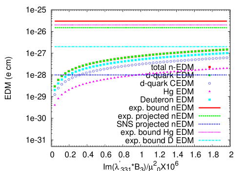
Figure 2: (color online) The neutron EDM (in units of e.cm) versus the combination $\Im(B_{3}^{\ast}\lambda^{\prime}_{331})$ normalized by $\mu_{\scriptscriptstyle 3}^{2}$.The horizontal lines show present EDM bounds as well as improvements possible in the future experiments.red solid line is current experimental bound for neutron EDM nEDM-recent , pink dotted line is current experimental bound for mercury EDM Hg-bound , green dashed line is the goal expected to be reached by the current Grenoble neutron EDM experiment nEDM-goal , cyan dash-dotted line is the expected measurement of of the proposed deuteron EDM experiment dt-edm-proposal , and blue hashed line is the expected improvement at the proposed Los Alamos neutron EDM experiment nEDM-SNS . The red filled squares stand for the total neutron EDM prediction, green filled circles are d-quark EDM, blue open circles are d-quark CEDM, cyan filled squares are predictions for deuteron EDM and magenta filled triangles are predictions for mercury EDM, in the present framework described in the previous section.

In Fig.(2) we have plotted the neutron, deuteron, and mercury EDMs, as well as d-quark EDM and CEDM, against the most important combination ${\rm Im}(B_{3}^{\ast}\lambda^{\prime}_{331})$ normalized by $\mu_{\scriptscriptstyle 0}^{2}$. This combination has the largest impact owing to top Yukawa and top mass dependence. We have not plotted u-quark EDM as it is about 5 orders of magnitude smaller than d-quark EDM (reflecting up-top hierarchy). The description of various lines and symbols is given in the caption for the figure. It is straight forward to understand the features of the plot. From the Eqs.(4) and (5, given that loop functions $F_{3}\approx F_{4}$ for the parameters considered here, one can see that $d^{\!\scriptscriptstyle E}_{d}/d^{\!\scriptscriptstyle C}_{d}\approx 5/(2\,g_{s})\approx 2.5$. This can be roughly observed in the plot. The plot also shows that total neutron EDM is same as the d-quark EDM contribution. To understand this, observe that u-quark EDM is negligible and hence the total neutron EDM is sum of d-quark EDM and CEDM. CEDM suffers not only a factor of 2.5 suppression as discussed above, but also has additional $e/4\pi$ suppression, which more than compensates QCD enhancement factor of 3.4. For d-quark EDM contribution, QCD suppression factor is compensated by the Clebsch-Gordan coefficient factor of $4/3$ and the total neutron EDM works out to be roughly same as d-quark EDM. In the similar way one can see from the formulas for deuteron and mercury EDMs that $d_{Hg}\approx d^{\!\scriptscriptstyle C}_{d}/3.14$ and $d_{\mathrm{deuteron}}=1.6\times d^{\!\scriptscriptstyle C}_{d}$. All these relations are born out in the plot.

Coming to bounds, from Fig.2, we see that the null result at the proposed Los Alamos EDM experiment can lead to a particularly stringent constraint on ${\rm Im}(B_{3}^{\ast}\lambda^{\prime}_{331})/\mu_{\scriptscriptstyle 0}^{2}<1.4\times 10^{-7}$. For the same combination the bound we obtain from the sensitivity of the proposed deuteron EDM experiment is $4.0\times 10^{-6}$ and from the present best limits on neutron EDM and Hg EDM experiment, $4.0\times 10^{5}$ and $1.9\times 10^{-4}$ respectively. This gives us an idea about the unprecedented sensitivity of the proposed Los Alamos neutron EDM experiment and the deuteron EDM experiment.

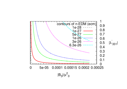
Figure 3: A contour plot for various values of neutron EDM in e.cm in the plane of real $\lambda^{\prime}_{331}$ and $B_{3}$. (with a relative phase of $\pi/4$). Cyan dash-dotted line is the previous best experimental bound, pink dotted line is the current best bound, blue hashed line is the expected reach of Grenoble experiment, black dashed line is the Los Alamos projected sensitivity. One can see a sizable improvement in the regions ruled out in parameter space with improvement in sensitivity.

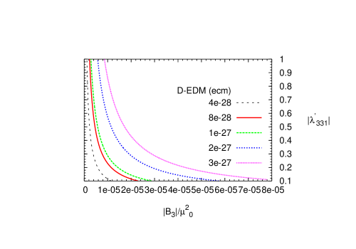
Figure 4: A contour plot for various values of deuteron EDM in e.cm in the plane of real $\lambda^{\prime}_{331}$ and $B_{3}$ (with a relative phase of $\pi/4$). Region between pink dotted line and green dashed line is the expected sensitivity of the proposed deuteron experiment. Black dashed line shows a possible order of magnitude improvement in this. Again one can see that any null result can rule out huge regions in parameter space.

Fig.3 shows the contours of neutron EDM in the plane of magnitudes for the couplings $\lambda^{\prime}_{331}$ and $B_{3}$ with the relative phase fixed at $\pi/4$. The contour for present experimental bound is shown in pink dotted line. The plot shows that a sizable region of the parameter space are ruled out. Successive contours show smaller values of neutron EDM with the smallest being $10^{-28}$ $e$ cm, the projected sensitivity of Los Alamos experiment. Fig.4 shows the contours of deuteron EDM in the plane of magnitudes for the couplings $\lambda^{\prime}_{331}$ and $B_{3}$ with the relative phase fixed at $\pi/4$. Region between pink dotted line and green dashed line is the expected sensitivity of the proposed deuteron experiment. Black dashed line shows a possible order of magnitude improvement in this. One can see that any null result can rule out huge regions in parameter space.

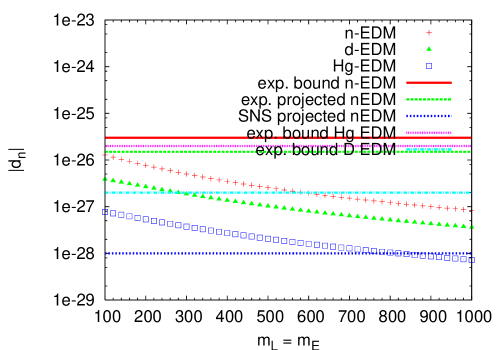
Figure 5: Various EDMs vs. the slepton mass parameter ${\tilde{m}}_{L}={\tilde{m}}_{E}$ (with $|B_{3}|=200~{}\mbox{GeV}^{2}$, $|\lambda^{\prime}_{331}|=.05$ and relative phase of $\pi/4$). Horizontal lines are the experimental bounds.

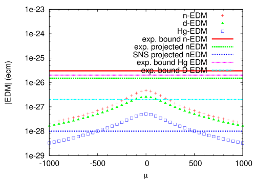
Figure 6: Various EDMs vs. $\mu_{\scriptscriptstyle 0}$ parameter with $|B_{3}|=200~{}\mbox{GeV}^{2}$, $|\lambda^{\prime}_{331}|=.05$ and relative phase $\pi/4$. Horizontal lines are the experimental bounds.

So far we have kept certain parameters like the phase of the RPV combination, the $\mu_{\scriptscriptstyle 0}$ parameter and the slepton mass spectrum fixed. To get a better understanding of the allowed regions in the overall parameter space, let us focus on variations of the parameters one at a time. In Fig.(5) we have plotted neutron EDM versus the slepton mass parameter ${\tilde{m}}_{L}={\tilde{m}}_{E}$ (with $|B_{3}|=200~{}\mbox{GeV}^{2}$, $|\lambda^{\prime}_{331}|=.05$ and relative phase of $\pi/4$). As expected the neutron EDM falls with the increasing slepton mass. More careful checking reveals that the result is sensitive only to one slepton mass parameter, the mass of the third $L$-handed slepton here. It is also easy to understand from our analytical formulas that the dominating contributions among the various scalar mass eigenstates for the case of $B_{i}^{\ast}\lambda^{\prime}_{ijk}$ come from the $i$-th $L$-handed slepton and the Higgs. Various horizontal lines are the experimental bounds. It is interesting to note that even if slepton mass is as high as 1 TeV, it still gives neutron EDM contribution that is an order of magnitude larger than the Los Alamos experiment sensitivity. In Fig.(6) we have shown the variation of neutron EDM with the $\mu_{\scriptscriptstyle 0}$ parameter. Although parameter $\mu_{\scriptscriptstyle 0}$ does not directly figure in the EDM formula, its influence is felt through the Higgs spectrum. Larger $\mu_{\scriptscriptstyle 0}$ leads to heavier Higgs spectrum which suppresses the EDM contribution. Again, it is interesting to see that $\mu{\scriptscriptstyle 0}=1$TeV, still gives neutron EDM contribution that is larger than the sensitivity of Los Alamos experiment. The large value of neutron EDM (much larger than the reach of Los Alamos experiment) even for slepton mass and $\mu_{\scriptscriptstyle 0}$ parameter at $1$ TeV is not only encouraging but also indicates that if a non-zero EDM is measured, one should exercise caution in the interpretation in terms of any new physics model. Our analytical formulas show that there is no strong dependence on $\tan\!\beta$ (we have checked this numerically as well) and hence we have kept $\tan\!\beta=3$ fixed in all the plots. Relative insensitivity to the value of $\tan\!\beta$ here can be contrasted to certain interesting predictions like Branching fraction for $B_{s}\to\mu^{+}\mu^{-}$ in MSSM which is boosted by three orders of magnitude in large $\tan\!\beta$ region. Any constraints on $\tan\!\beta$ following non-observations of $B_{s}\to\mu^{+}\mu^{-}$ would still leave our predictions unaffected. The fact that our predictions largely depend on hitherto unconstrained combination $B_{i}^{*}\lambda^{\prime}_{ij1}$ and already known top Yukawa and top mass, makes it all the more interesting.

To go beyond the illustrative case of the parameter combination $B_{i}^{\ast}\lambda^{\prime}_{i31}$ , we list in table 1 the bounds due to the neutron EDM from the current Grenoble results (in the column under I), due to plausible null result at Los Alamos experiment (in the column under II), as well as due to any null results of the future deuteron EDM experiment (in the column under III), on the nine combinations $|B_{i}^{\ast}\lambda^{\prime}_{ij1}|$ normalized by $(100~{}\mbox{GeV})^{2}$. It is interesting to note the difference in bounds for case (a) and (b) for coupling combination $|B_{i}^{\ast}\lambda^{\prime}_{i31}|$ and $|B_{i}^{\ast}\lambda^{\prime}_{i21}|$. The inputs for Case (b) are identical to case (a) except for RPV phase being zero for case (b). Case (b) thus relies solely on CKM phase. Interestingly the bound for $|B_{i}^{\ast}\lambda^{\prime}_{i31}|$ changes very marginally from case (a) to (b) whereas the bound for $|B_{i}^{\ast}\lambda^{\prime}_{i21}|$ weakens by about an order of magnitude. To understand this difference in behavior of $|B_{i}^{\ast}\lambda^{\prime}_{i31}|$ and $|B_{i}^{\ast}\lambda^{\prime}_{i21}|$, with and without a complex phase in the RPV couplings, we have plotted in Fig. 7 the allowed region in the plane of relative phase of $B^{\ast}_{3}\lambda^{\prime}_{331}$ and the $|B^{\ast}_{3}\lambda^{\prime}_{331}|$ (left) and relative phase of $B^{\ast}_{3}\lambda^{\prime}_{321}$ and the $|B^{\ast}_{3}\lambda^{\prime}_{321}|$ (right). One can see that the bound for $|B^{\ast}_{3}\lambda^{\prime}_{331}|$ is about the same for relative phase in $B^{\ast}_{3}\lambda^{\prime}_{331}$ of 0 or $\pi/4$ but the bound for $|B^{\ast}_{3}\lambda^{\prime}_{321}|$ strengthens by about an order of magnitude as the phase in the RPV coupling increases from 0 to $\pi/4$ suggesting a collaborative effect between the CKM phase and the RPV phase. Fig.8 is similar to Fig.7 except that it is now for deuteron EDM. We see that a similar pattern here also because of the similar qualitative dependence on down-quark EDM, implying similar interference pattern between CKM phase and RPV phase induced contributions. For the case of $B_{i}^{\ast}\lambda^{\prime}_{i11}$ there is no CKM phase involved. In the table we have fixed the sign of $\mu_{\scriptscriptstyle 0}$ parameter to be negative. In the Fig.6 it is seen that absolute value of neutron EDM is symmetric with respect to sign of $\mu_{\scriptscriptstyle 0}$ parameter and hence positive $\mu_{\scriptscriptstyle 0}$ should give identical bounds. The variation of bounds in table 1 with changes in parameters $\mu_{\scriptscriptstyle 0}$ and the slepton and Higgs mass very much follows the pattern found in plots discussed earlier.

Table 1: Here we list the normalized upper bounds for several combinations of bilinear and trilinear RPV parameters, with some variation in the input parameters. The bounds essentially depend on the values of parameters like ${\tilde{m}}_{\scriptscriptstyle L},\mu_{\scriptscriptstyle 0}$ and $m_{{\scriptscriptstyle H}_{d}}$ ($m_{{\scriptscriptstyle H}_{u}}$ and $B_{0}$ being determined from EW symmetry breaking condition). $\tan\!\beta$ has been kept fixed at 3 as EDM has a very mild dependence on $\tan\!\beta$. Note that all these bounds include CEDM contributions. Columns headings I,II,III refer to bounds from current neutron EDM experiment, from the possible null results at the Los Alamos neutron EDM experiment, and the possible null results at the deuteron EDM experiment respectively. As is clearly seen, any null results at Los Alamos experiment can lead to bounds that are over two orders of magnitude larger than the current bounds

parameter values					Normalized bounds
	$\mu_{\scriptscriptstyle 0}$	${\tilde{m}}_{\scriptscriptstyle L}$	$m_{{\scriptscriptstyle H}_{d}}$	RPV	$\frac{\Im(B_{i}^{\ast}\cdot\lambda^{\prime}_{i31})}{(100~{}\mbox{GeV})^{2}}$			$\frac{\Im(B_{i}^{\ast}\cdot\lambda^{\prime}_{i21})}{(100~{}\mbox{GeV})^{2}}$			$\frac{\Im(B_{i}^{\ast}\cdot\lambda^{\prime}_{i11})}{(100~{}\mbox{GeV})^{2}})$
	(GeV)	(GeV)	(GeV)	phase	I	II	III	I	II	III	I	II	III
(a)	-100	100	100	$\pi/4$	$1.5\cdot 10^{-4}$	$5.0\cdot 10^{-7}$	$1.5\cdot 10^{-5}$	$4.3\cdot 10^{-4}$	$1.3\cdot 10^{-6}$	$2.5\cdot 10^{-5}$	$1.7\cdot 10^{-3}$	$5.2\cdot 10^{-6}$	$1.1\cdot 10^{-4}$
(b)	-100	100	100	0	$8.0\cdot 10^{-5}$	$2.5\cdot 10^{-7}$	$2.0\cdot 10^{-5}$	$2.0\cdot 10^{-3}$	$6.5\cdot 10^{-6}$	$5.1\cdot 10^{-4}$	nil	nil	nil
(c)	-400	100	100	$\pi/4$	$5.5\cdot 10^{-4}$	$2.6\cdot 10^{-6}$	$5.2\cdot 10^{-5}$	$2.7\cdot 10^{-4}$	$9.2\cdot 10^{-6}$	$1.6\cdot 10^{-4}$	$1.0\cdot 10^{-2}$	$3.5\cdot 10^{-5}$	$6.6\cdot 10^{-4}$
(d)	-800	100	100	$\pi/4$	$1.7\cdot 10^{-3}$	$5.5\cdot 10^{-5}$	$1.5\cdot 10^{-4}$	$9.0\cdot 10^{-3}$	$3.0\cdot 10^{-5}$	$5.4\cdot 10^{-4}$	$3.2\cdot 10^{-2}$	$1.1\cdot 10^{-4}$	$2.1\cdot 10^{-3}$
(e)	-100	400	100	$\pi/4$	$6.3\cdot 10^{-4}$	$2.1\cdot 10^{-6}$	$5.6\cdot 10^{-5}$	$4.2\cdot 10^{-3}$	$1.5\cdot 10^{-5}$	$2.6\cdot 10^{-4}$	$1.5\cdot 10^{-2}$	$5.2\cdot 10^{-5}$	$1.1\cdot 10^{-3}$
(f)	-100	800	100	$\pi/4$	$1.9\cdot 10^{-3}$	$6.4\cdot 10^{-6}$	$1.6\cdot 10^{-4}$	$1.5\cdot 10^{-2}$	$5.2\cdot 10^{-5}$	$9.2\cdot 10^{-4}$	$5.1\cdot 10^{-2}$	$1.8\cdot 10^{-4}$	$3.6\cdot 10^{-3}$
(g)	-100	100	300	$\pi/4$	$3.8\cdot 10^{-4}$	$1.2\cdot 10^{-6}$	$3.6\cdot 10^{-5}$	$1.7\cdot 10^{-3}$	$6.0\cdot 10^{-6}$	$1.0\cdot 10^{-4}$	$6.6\cdot 10^{-3}$	$2.3\cdot 10^{-5}$	$4.2\cdot 10^{-4}$
(h)	-100	100	600	$\pi/4$	$1.0\cdot 10^{-3}$	$3.5\cdot 10^{-6}$	$9.2\cdot 10^{-5}$	$5.8\cdot 10^{-3}$	$2.0\cdot 10^{-5}$	$3.5\cdot 10^{-4}$	$2.1\cdot 10^{-2}$	$7.6\cdot 10^{-5}$	$1.4\cdot 10^{-3}$

Before we conclude, we would like to briefly comment on two things. In the table 1, we have only mentioned the bounds for the nine combinations $|B_{i}^{\ast}\lambda^{\prime}_{ij1}|$, whereas earlier in the text we did mention that in principle all the twenty-seven $\lambda^{\prime}_{ijk}$ together with bilinear couplings do contribute to the neutron EDM. The couplings other than $\lambda^{\prime}_{ij1}$ contribute to $u$ quark EDM and all the contributions are proportional to up-Yukawa (in contrast to the presence of a contribution proportional to top-Yukawa for the $d$ quark EDM). Strength of the corresponding contributions is substantially weaker (typically by 5 to 6 orders of magnitude) and hence do not lead to meaningful bounds. The other thing is about the possible $\mu_{i}^{\ast}\cdot\lambda^{\prime}_{ijk}$ contributions. It can be seen in Eq.(29) that these are second order in perturbation and also accompanied by lepton mass $\mu_{i}$. Thus, a typical $\mu_{i}^{\ast}\lambda^{\prime}_{ijk}$ contribution is substantially weaker than the corresponding $B_{i}^{\ast}\lambda^{\prime}_{ijk}$ contribution. For instance, with the similar inputs for other SUSY parameters as described above, if one takes $\mu_{3}=10^{-3}$ GeV (dictated by requirement of sub-ev neutrino masses), $\lambda^{\prime}_{331}=.05$ and a relative phase of $\pi/4$, one obtains neutron EDM of $6.0\cdot 10^{-32}$ which is about six orders of magnitude smaller than the present experimental bound on neutron EDM. If one goes by the upper bound on the mass of $\nu_{\tau}$ of 18.2 MeV nu_mass , $\mu_{\scriptscriptstyle 3}$ could be as large as 7 GeV for $\tan\!\beta=2$ and sparticle mass $\sim 300$ GeV ru2 . For $\mu_{\scriptscriptstyle 3}=1$ GeV we obtain neutron EDM of $6.1\cdot 10^{-29}$, still about three orders of magnitude smaller than the experimental bound. These numbers can be easily compared with the $\mu^{\ast}_{i}\lambda^{\prime}_{i11}$ contributions to the $d$ quark EDM through chargino loop in Table 1 of ref.nedm . There the corresponding contribution (with $\mu_{\scriptscriptstyle 3}=1$ GeV) is much weaker (of order $10^{-32}$) as it lacks the top Yukawa and top mass enhancements. In the same table one finds that corresponding contribution to gluino loop is much stronger (of order $10^{-25}$) due to proportionality to gluino mass and strong coupling constant. In the light of above reasons one can appreciate that the contributions due to soft parameter $B_{i}$ are far more dominating in the present scenario of quark loop contributions.

V Conclusions

We have made a systematic study of the influence of the combination of bilinear and trilinear RPV couplings on the neutron, deuteron, and mercury EDMs, including the contributions from chromo-electric dipole form factor. Such combinations are interesting because this is the only way RPV parameters contribute at one-loop level to EDM. The fact that the form factors are proportional to top Yukawa and top mass with the hitherto unconstrained combination of RPV parameters, makes them all the more interesting. Such class of diagrams have a quark as the fermion running inside the loop. EDMs of neutron, deuteron, and mercury are ultimately expressed in terms of quark EDMs and CEDMs. In our analytical expressions obtained based on perturbative diagonalization of the scalar mass-squared matrices, we demonstrated that charged-slepton Higgs mixing loop contribution to $d$ quark EDM far dominates the other contributions due to a diagram with the top-quark in the loop. In our numerical exercise we have obtained robust bounds on the combinations $\frac{{\rm Im}(B_{i}^{\ast}\cdot\lambda^{\prime}_{ij1})}{(100~{}\mbox{GeV})^{2}}$ for $i,j=1,2,3$ that have not been reported before. The bounds are reported for the current best limits on neutron EDM as well as projected for any null results in the future improvements at Grenoble and Los Alamos experiments as well as deuteron EDM experiment. It turns out that measurements of mercury EDM are not as strongly constraining as current neutron EDM limits, whereas any null result at deuteron EDM and/or Los Alamos neutron EDM experiment can lead to much stronger constraints on RPV parameter space (for instance${\rm Im}(B_{3}^{\ast}\lambda^{\prime}_{331})/\mu_{\scriptscriptstyle 0}^{2}<1.4\times 10^{-7}$). Even if the RPV couplings are real, they could still contribute to quark EDMs via CKM phase. For some cases CKM phase induced contribution is as strong as that due to an explicit complex phase in the RPV couplings. We find that even if slepton mass or $\mu_{\scriptscriptstyle 0}$ are as high as 1 TeV, it could still lead to bounds that are well within the reach of Los Alamos neutron EDM experiment. There also exist contributions involving $\mu_{i}^{\ast}\lambda^{\prime}_{ijk}$. However these are higher order effects which are further suppressed by proportionality to charged lepton mass. Since $\mu_{i}$ are expected to be very small (of order $10^{-3}$ GeV) for sub-eV neutrino masses, such contributions are highly suppressed. Our results presented here make available a new set of interesting bounds on combinations of RPV parameters.

One further thing worth some attention here is the question of to what extent our choice of model formulas for the hadronic EDMs from quark dipoles, as discussed and justified above, affect our major conclusions . One can think about presenting full numerical results and comparison for the cases of the various different model formulas. However, we find that neither feasible nor desirable. We did do some numerical checking, but consider a brief summary here as the only appropriate thing to present. Two special features of the RPV model dictate the answer. The hadron EDMs are to be determined from the EDMs and CEDMs of the $u$, $d$, and $s$ quark. For the RPV model, the resulted dipoles for $u$-quark are much smaller than of the $d$-quark. For the $s$-quark, however, dominant contributions involve similar diagrams with trilinear RPV couplings of different familiy indices, typically replacing a $1$ for the $d$ by a $2$ for the $s$. The latter complicaton makes it difficult to fully address the impact within the scope of the present study. However, one can at least see that for the RPV parameter combinations playing a dominant role in generating $d$ dipoles, our main focus here, their contributions to the $s$ dipoles are going to be unimportant. Neglecting the the $s$ and $u$ dipoles, models formulas from QCD sum rule and the valence quark model give roughly $d_{n}\simeq 0.92\,d_{d}^{\!\scriptscriptstyle E}$ and $d_{n}\simeq 0.96\,d_{d}^{\!\scriptscriptstyle E}$, respectively. The case for comparison with the chiral lagrangian approach is more complicated. But the result agrees within a factor of three with the two numbers. The deuteron EDM numbers from the two approaches agree within error bars. And the Mercury EDM constraint is always negligible when compared to that of neutron and Deuteron, even when $s$ dipoles are to be considered. Hence, our results here are not much affected by the hadron EDMs model formulas chosen.

Figure 1: $d$ quark EDM due to $B^{\ast}_{i}\lambda^{\prime}_{i31}$ combination. Due to top Yukawa and top-mass dependence this is the most dominant contribution.

Figure 7: Dotted region is the parameter space allowed by neutron EDM upper bound in the plane of relative phase of $\lambda^{\prime}_{331}B^{\ast}_{3}$ and the $|\lambda^{\prime}_{331}B^{\ast}_{3}|$ (top) and relative phase of $\lambda^{\prime}_{321}B^{\ast}_{3}$ and the $|\lambda^{\prime}_{321}B^{\ast}_{3}|$ (bottom).

Figure 8: Dotted region is the parameter space allowed by proposed deuteron EDM upper bound in the plane of relative phase of $\lambda^{\prime}_{331}B^{\ast}_{3}$ and the $|\lambda^{\prime}_{331}B^{\ast}_{3}|$ (top) and relative phase of $\lambda^{\prime}_{321}B^{\ast}_{3}$ and the $|\lambda^{\prime}_{321}B^{\ast}_{3}|$ (bottom).

References

- (1) J. H. Christenson, J. W. Cronin, V. L. Fitch, and R. Turlay, Phys. Rev. Lett. 13, 138 (1964).
- (2) B. Aubert et al. [BABAR Collaboration], Phys. Rev. Lett. 87, 091801 (2001); K. Abe et al. [Belle Collaboration], Phys. Rev. Lett. 87, 091802 (2001).
- (3) L. Landau, Nucl. Phys. 3, 127 (1957).
- (4) M. Pospelov and A. Ritz, Annals of Physics 318, 119 (2005).
- (5) J.S.M. Ginges and V.V. Flambaum, Phys. Rep. 397, 63 (2004).
- (6) E. Purcell and N. Ramsey Phys. Rev. 78, 807 (1950).
- (7) E. E. Salpeter Phys. Rev. 112, 1642 (1958).
- (8) P.G.H. Sanders Phys. Lett. 14, 194 (1965).
- (9) B. C. Regan et al. Phys. Rev. Lett. 88, 071805 (2002).
- (10) M. Romalis et al. Phys. Rev. Lett. 86, 2505 (2001).
- (11) Fortson’s talk at Lepton-Moments, Cape Cod, 9-12 June 2003, http:g2pcl.bu.edu/ leptonmom/program.html
- (12) P. G. Harris et al., Phys. Rev. lett. 82, 904 (1999).
- (13) C.A. Baker et al. hep-ex/0602020.
- (14) V. der Grinten, talk at Lepton-Moments, Cape Cod, 9-12 June 2003.
- (15) http://p25ext.lanl.gov/edm/edm.html
- (16) F.J.M. Farley et al. Phys. Rev. Lett 93, 052001 (2004).
- (17) Y. K. Semertzidis et al. hep-ph/0012087, Proceedings of HIMUS99 Workshop, Tsukuba, Japan (1999).
- (18) For J-PARK letter of intent, please see http://www.bnl.gov/edm/papers/jpark_loi_030109.pdf .
- (19) For deuteron EDM proposal, please see http://www.bnl.gov/edm/deuteron_proposal_040816.pdf
- (20) M. Bisset, O.C.W. Kong, C. Macesanu, L.H. Orr, Phys. Lett. B430, 274 (1998); Phys. Rev. D62, 035001 (2000).
- (21) O.C.W. Kong, Int. J. Mod. Phys. A19, 12 (2004).
- (22) For neutrino masses from R-parity Violation, see for example S.K. Kang and O.C.W. Kong Phys. Rev. D69, 013004 (2004); O. C. W. Kong JHEP 0009,037 (2000); A.S. Joshipura, R.D. Vaidya and S.K. Vempati Nucl. Phys. B639, 290 (2002); Phys. Rev. D65, 053018 (2002).
- (23) A.S. Joshipura, R.D. Vaidya and S.K. Vempati Phys. Rev. D62, 093020 (2000).
- (24) E. Shabalin Sov. Phys. Usp. 26, 297 (1983), Usp. Fiz. Nauk.139, 561 (1983); M.E. Pospelov Phys. Lett. B328 , 441 (1994); I.B. Khriplovich and A. R. Zhitnitsky, Phys. Lett. B109 , 490 (1982).
- (25) R. Arnowitt, J. L. Lopez and D. V. Nanopoulos, Phys. Rev. D42, 2423 (1990).
- (26) See for example Y. Kizukuri and N. Oshimo Phys. Rev. D 46, 3025 (1992).
- (27) T. Ibrahim and P. Nath Phys. Rev. D 58, 111301 (1998).
- (28) T. Kadoyoshi and N. Oshimo Phys. Rev. D 55, 1481 (1997). bartl-D99 A. Bartl, T. Gajdosik, W. Porod, P. Stockinger and H. Stremnitzer, Phys. Rev. D, 073003 (1999).
- (29) U. Chattopadhyay, T. Ibrahim and D.P. Roy Phys. Rev. D64, 013004 (2001).
- (30) T. Falk and K.A. Olive, Phys. Lett. B439, 71 (1998).
- (31) J. Hisano and Y. Shimizu, Phys. Rev. D70, 093001 (2004).
- (32) M. Pospelov and A. Ritz, Phys. Rev. D63, 073015 (2001).
- (33) D.A. Demir and Y. Farzan, JHEP 10, 068 (2005)
- (34) G. Degrassi, E. Franco, S. Marchetti, L. Silvestrini, JHEP 11, 44 (2005).
- (35) S.Y. Ayazi and Y. Farzan hep-ph/0605272.
- (36) R.M. Godbole, S. Pakvasa, S.D. Rindani, and X. Tata, Phys, Rev. D 61, 113003 (2000); S.A. Abel, A. Dedes and H.K. Dreiner J. High Energy Phys.05, 013 (2000). Also see, D. Chang, W.-F. Chang, M. Frank, and W.Y. Keung, Phys. Rev. D62, 095002 (2000).
- (37) Y.-Y. Keum and O.C.W. Kong, Phys, Rev. Lett. 86, 393 (2001); Phys, Rev. D 63, 113012 (2001).
- (38) K. Choi, E.J. Chun, K. Hwang, Phys, Rev. D63, 013002 (2001).
- (39) O.C.W. Kong and R.D. Vaidya, Phys. Rev. D72, 014008 (2005); see also O.C. .W. Kong and R.D. Vaidya, Phys. Rev. D71, 055003 (2005).
- (40) K.Cheung and O.C.W. Kong Phys. Rev. D64, 095007 (2001).
- (41) M. Chemtob Prog. Part. Nucl. Phys. 54, 71 (2005).
- (42) T. Falk, K. Olive, M. Pospelov and R. Roiban, Nucl. Phys. B560, 3 (1999).
- (43) J. Hisano, M. Kakizaki, M. Nagai and Y. Shimizu, Phys. Lett. B604, 216 (2004).
- (44) M. Pospelov, Phys. Lett. B530, 123 (2002).
- (45) O. Lebedev, K. Olive, M. Pospelov and A. Ritz, Phys. Rev. D70, 016003 (2004).
- (46) J. Hisano and Y. Shimizu, Phys. Rev. D70 , 093001 (2004).
- (47) R. Barate et al. , Eur. Phys. J. C2, 395 (1998).