A convexity theorem for real projective structures

Abstract

Given a finite collection $\mathcal{P}$ of convex $n$-polytopes in $\mathbb{R}\textup{P}^{n}$ ($n\geq 2$), we consider a real projective manifold $M$ which is obtained by gluing together the polytopes in $\mathcal{P}$ along their facets in such a way that the union of any two adjacent polytopes sharing a common facet is convex. We prove that the real projective structure on $M$ is

1. convex if $\mathcal{P}$ contains no triangular polytope, and

2. properly convex if, in addition, $\mathcal{P}$ contains a polytope whose dual polytope is thick.

Triangular polytopes and polytopes with thick duals are defined as analogues of triangles and polygons with at least five edges, respectively.

1 Introduction

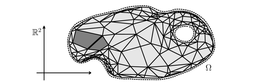
Figure 1.1: A feasible picture of a planar domain $\Omega$ with a residually convex tessellation. Shaded is the union of two polygons sharing the thick common edge.

Consider a planar domain $\Omega$, an open connected subset of $\mathbb{R}^{2}$. Suppose that $\Omega$ admits a tessellation $\mathcal{T}$ by (a necessarily infinite number of) convex polygons. One may ask if there are any local conditions on the tessellation $\mathcal{T}$ which can guarantee convexity of the domain $\Omega$. One reasonable such condition we investigate in this paper is the following:

the union of two adjacent polygons sharing a common edge is convex.

See Figure 1.1. This condition was first introduced by Kapovich [11] and we call tessellations with this property residually convex. It turns out that, under the residual convexity condition, one can prove the following:

1. If $\mathcal{T}$ contains no triangle then the domain $\Omega$ is a convex subset of $\mathbb{R}^{2}$.

2. If, in addition, $\mathcal{T}$ contains a polygon with at least $5$ edges then the convex domain $\Omega$ contains no infinite line.

Figure 1.2 illustrates the above assertions: (a) exhibits a generic shape of a convex domain which admits a residually convex tessellation without triangles, (b) shows that a domain containing an infinite line may admit a residually convex tessellation without polygons with at least $5$ edges, and (c) shows that a domain with residually convex tessellation containing a pentagon but no triangles is bounded.

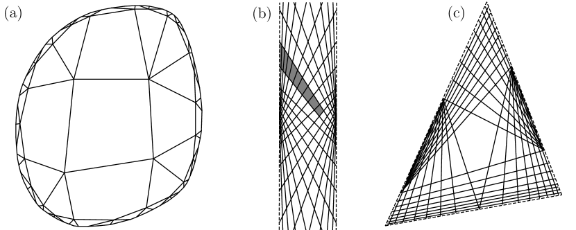
Figure 1.2: (a) A generic residually convex tessellation without triangles. (b) An unbounded domain with residually convex tessellation by quadrilaterals, which is not the standard tessellation of $\mathbb{R}^{2}$ by squares. A directed gallery (see Definition 5.9) is shaded. (c) A maximal domain with residually convex tessellation containing the pentagon in the middle but no triangles.

On the other hand, Figure 1.3 (b) shows that a non-convex domain may admit a residually convex tessellation if triangles are allowed. Figure 1.3 (a) motivated the definition of residual convexity because it clearly exhibits one way in which a non-convex domain may be tessellated by convex polygons. Both examples are due to Yves Benoist.

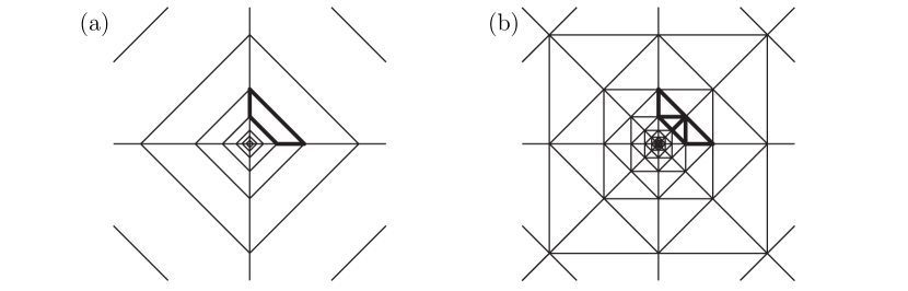
Figure 1.3: (a) Given a quadrilateral $P\subset\mathbb{R}^{2}$ with vertices $(1,0),(2,0),(0,1)$ and $(0,2)$, a tessellation of $\mathbb{R}^{2}\setminus\{0\}$ is obtained by taking orbits of $P$ under the action of the group generated by the homothety by $2$ and the rotation by $\pi/2$. (b) A residually convex tessellation of $\mathbb{R}^{2}\setminus\{0\}$ by triangles is obtained by decomposing the quadrilateral $P$ in (a) into four triangles.

Our contribution in this paper is to prove the assertions similar to (I) and (II) above in every dimension – by defining appropriate analogues of triangles and polygons with at least $5$ edges. The former is called a triangular polytope and the latter has a thick polytope as its dual. For precise definitions see Definition 4.11 and Definition 5.2. As a matter of fact, we prove these results in a more general context so that they give rise to convexity criteria for certain real projective structures. From now on, to the end of the paper, we assume $n\geq 2$ except those cases which are trivially exceptional (like the one in the next paragraph).

A real projective structure on manifolds is a geometric structure which is locally modelled on projective geometry $(\mathbb{R}\textup{P}^{n},\textup{Aut}(\mathbb{R}\textup{P}^{n}))$. If $\Omega\subset\mathbb{R}\textup{P}^{n}$ is a convex domain and $\Gamma$ is a discrete subgroup of $\textup{Aut}(\mathbb{R}\textup{P}^{n})$ acting freely and properly discontinuously on $\Omega$, then the induced real projective structure on the quotient manifold $\Omega/\Gamma$ is said to be convex. If, moreover, the closure of the convex domain $\Omega$ does not contain any projective line, then the structure is called properly convex. See Section 6.1 for more details. One of the basic references for real projective structures is the lecture notes of Goldman [7].

Convex real projective structures can be regarded as analogues of complete Riemannian metrics, and properly convex real projective structures are expected to share some nice properties with non-positively curved metrics (see, for example, [1] and [2]). For this reason, given a real projective structure, one natural question to ask is whether the structure is (properly) convex. More precisely, let $\{P_{i}\}$ be a finite family of convex $n$-dimensional polytopes in $\mathbb{R}\textup{P}^{n}$. Suppose that $M$ is a real projective $n$-manifold obtained by gluing together copies of $P_{i}$ via projective facet-pairing transformations. Then there is an associated developing map $dev:\tilde{M}\to\mathbb{R}\textup{P}^{n}$ of the universal cover $\tilde{M}$ of $M$, which is a projective isomorphism on each cell of $\tilde{M}$. One now asks:

When is the map $dev$ an isomorphism onto a (properly) convex domain in $\mathbb{R}\textup{P}^{n}$?

The Tits–Vinberg fundamental domain theorem [16] for discrete linear groups generated by reflections provides a rather restricted but very constructive solution to this question. Recently Kapovich [11] proved another convexity theorem when the $P_{i}$ are non-compact polyhedra. See Remark 6.3 for a more detailed discussion. In the present paper, we deal with complementary cases which are not covered by the aforementioned results. Our main theorem is as follows (see also Theorem 6.2):

Theorem A.

Let $\mathcal{P}$ be a finite family of compact convex $n$-dimensional polytopes in $\mathbb{R}\textup{P}^{n}$. Let $\Phi=\{\phi_{\sigma}\in\textup{Aut}(\mathbb{R}\textup{P}^{n})\,|\,\sigma\in\Sigma\}$ be a set of projective facet-pairing transformations for $\mathcal{P}$ indexed by the collection $\Sigma$ of all facets of the polytopes in $\mathcal{P}$. Let $M$ be a real projective $n$-manifold obtained by gluing together the polytopes in $\mathcal{P}$ by $\Phi$. Assume the following condition:

for each facet $\sigma$ of $P\in\mathcal{P}$, if $\sigma^{\prime}$ is a facet of $P^{\prime}\in\mathcal{P}$ such that $\phi_{\sigma}(\sigma)=\sigma^{\prime}$, then the union $\phi_{\sigma}(P)\cup P^{\prime}$ is a convex subset of $\mathbb{R}\textup{P}^{n}$.

Then the following assertions are true:

1. If $\mathcal{P}$ contains no triangular polytope, then the developing map $dev:\tilde{M}\to\mathbb{R}\textup{P}^{n}$ is an isomorphism onto a convex domain which is not equal to $\mathbb{R}\textup{P}^{n}$;

2. If, in addition, $\mathcal{P}$ contains a polytope $P$ whose dual $P^{*}$ is thick, then the map $dev:\tilde{M}\to\mathbb{R}\textup{P}^{n}$ is an isomorphism onto a properly convex domain.

An interesting related question is whether every convex real projective structures have convex fundamental domains and how common residually convex structures are. In [12] we provide partial answer by showing that all properly convex real projective structures have convex fundamental domains.

1.1 Convexity

We sketch our approach to assertion (I) of Theorem A. The details are the contents of Section 3 and Section 4. Let $X=\tilde{M}$ denote the universal covering space of $M$. We consider the lift $dev:X\to\mathbb{S}^{n}$ of the developing map to the sphere $\mathbb{S}^{n}$, the two-fold cover of $\mathbb{R}\textup{P}^{n}$. Regarding $\mathbb{S}^{n}$ then as the standard Riemannian sphere, we pull back the Riemannian metric to $X$ via $dev$ so that $X$ is locally isometric to $\mathbb{S}^{n}$. Then the simply-connected manifold $X$ becomes a spherical polyhedral complex.

1. In fact, we define such a spherical polyhedral complex $X$ admitting a developing map $dev$ into $\mathbb{S}^{n}$ in an abstract way ($n$-complex), so that in general the complex $X$ does not necessarily admit a cocompact group action (see Definition 3.1). We call a subset $S\subset X$ convex if it is mapped by $dev$ injectively onto a convex subset of $\mathbb{S}^{n}$.

2. We then place on $X$ the residual convexity condition, that is, we require that, for every two $n$-polytopes $P_{1}$ and $P_{2}$ in $X$ sharing a common facet, their union $P_{1}\cup P_{2}$ be convex (see Definition 4.2).

3. We fix a polytope $P_{0}$ of $X$ and consider the iterated stars $st^{k}(P_{0})$ of $P_{0}$ so that they exhaust the whole complex $X$ (see Definition 3.5 (1)). Our plan is to show inductively that

   each star $st^{k}(P_{0})$ is convex and its image under $dev$ is not equal to $\mathbb{S}^{n}$.

   Then this would imply that $dev:X\to\mathbb{S}^{n}$ is an isometric embedding onto a convex proper domain in $\mathbb{S}^{n}$ (see Theorem 4.8).

4. Projecting $dev:X\rightarrow\mathbb{S}^{n}$ down back to $\mathbb{R}\textup{P}^{n}$ we get the desired convexity result on the real projective structure on $M$.

A considerable portion of the present paper is devoted to step (3) of the above plan. We now explain how the induction argument goes:

1. It turns out that the residual convexity establishes the base step of the induction (see Lemma 4.1 (1) and Lemma 3.6 (1)).

2. We assume that the $k$-th star $st^{k}(P_{0})$ is convex and its image under $dev$ is not equal to $\mathbb{S}^{n}$. Then it is rather easy to show that the $(k+1)$-th star $st^{k+1}(P_{0})$ is mapped injectively onto a topological ball ($n$-polyball) in $\mathbb{S}^{n}$ (see Lemma 3.6 (2) and Definition 3.3).

3. We next want to show that the star $st^{k+1}(P_{0})$ is locally convex. Because of its polyhedral structure, the local convexity of $st^{k+1}(P_{0})$ can be drawn from its local convexity near codimension-$2$ cells (ridges) in the boundary (see Lemma 3.4).

4. Let $e$ be a codimension-$2$ cell in the boundary of the star $st^{k+1}(P_{0})$. The local geometry of $st^{k+1}(P_{0})$ near $e$ is determined by the union $U(e)$ of $n$-cells in $X$ which contain $e$ and which intersect $st^{k}(P_{0})$. Thus we need to find conditions which imply that the union $U(e)$ is convex. Interestingly, there is a local condition for this.

5. Indeed, we consider a small neighborhood $res(e)$ (residue) of $e$ which consists of those $n$-cells in $X$ which contain $e$ (see Definition 3.5 (2)). Residual convexity implies that $res(e)$ is convex (see Lemma 4.1 (3)). Because the star $st^{k}(P_{0})$ is also assumed to be convex and because $st^{k}(P_{0})$ and $res(e)$ intersect along their boundaries, their intersection $F:=st^{k}(P_{0})\cap res(e)$ is a convex subset in the boundary of $res(e)$. Then the union $U(e)$ can be described as the union $U(e,F)$ of $n$-cells in $res(e)$ which intersect $F$.

6. The condition, which we call strong residual convexity, requires that, for all $e$, the set $U(e,F)$ be always convex regardless of convex subsets $F$ in the boundary of $res(e)$ (see Definition 4.4 and Definition 4.6). Figure 1.4 illustrates the case where strong residual convexity fails. In conclusion, under the assumption of strong residual convexity, we can show that the star $st^{k+1}(P_{0})$ is locally convex near codimension-$2$ cells in its boundary (see Lemma 4.7).

   

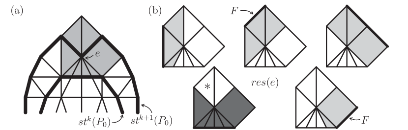
   Figure 1.4: Strong residual convexity. (a) A codimension-$2$ cell $e$ is in the boundary of $st^{k+1}(P_{0})$. The union of $n$-cells containing $e$ forms a convex neighborhood $res(e)$ of $e$, which intersects the convex set $st^{k}(P_{0})$ along its boundary. (b) The set $res(e)$ has five maximal convex subsets $F$ in its boundary. For one of such $F$, the union of $n$-cells of $res(e)$ intersecting $F$ is not convex. The corresponding picture is marked by (*).

7. Finally, once the local convexity is established, we may regard the star $st^{k+1}(P_{0})$ as an Alexandrov space of curvature $\geq 1$ and then deduce its global convexity using a well-known local-to-global theorem for such spaces (see Corollary 2.5). All induction steps are complete.

To summarize, we have the following convexity theorem:

Theorem B.

Let $X$ be an $n$-complex. If $X$ is strongly residually convex, then $X$ is isometric to a convex proper domain in $\mathbb{S}^{n}$. In particular, $X$ is contractible.

As can be seen in steps (iii)-(vi) above, the codimension-$2$ phenomena in polyhedral complexes enables us to go from dimension $2$ to arbitrary dimensions. This is a rather common trick which can be found, for example, in the proof of the Poincaré fundamental polyhedron theorem for constant curvature spaces (see, for example, [5] and [15]). However, we find it worthwhile to develop this trick into a form which is suitable for our present purpose. Hence the most of Section 2 is devoted to the study of geometric links of faces of various dimensions in convex polytopes.

Although strong residual convexity is entirely a local condition, for practical reasons, it is desirable to have simple combinatorial conditions under which residual convexity becomes strong residual convexity. Observe that triangles caused the failure of strong residual convexity in Figure 1.4. See also Figure 4.2. Using the codimension-$2$ phenomena once again, we define triangular polytopes and show that without presence of triangular polytopes residual convexity implies strong residual convexity (see Theorem 4.12). Combining this result with Theorem B we obtain the following corollary, which again implies assertion (I) of Theorem A.

Corollary C.

Let $X$ be a residually convex complex. If $X$ contains no triangular polytopes, then $X$ is isometric to a convex domain which is not $\mathbb{S}^{n}$.

1.2 Proper convexity

We now outline our approach to assertion (II) of Theorem A. The details are explained in Section 5. The starting point is the above Corollary C. That is, we assume that our complex $X$ is residually convex and contains no triangular polytopes. Then $X$ is isometric to a convex domain in $\mathbb{S}^{n}$. Thus from now on we regard $X$ as a convex subset of $\mathbb{S}^{n}$ and find conditions implying proper convexity of $X$.

Our eventual plan is to find $n+1$ supporting hyperplanes of $X$ that are in general position. Then $X$ is contained in the $n$-simplex which is determined by these hyperplanes. Because $n$-simplices are properly convex, the conclusion then follows. Fortunately, there is a natural way to find supporting hyperplanes of $X$ provided that $X$ contains no triangular polytope. Thus we need to find further conditions under which there are $n+1$ such in general position.

For example, if $X$ is $2$-dimensional and contains no triangle, all polygons in $X$ have at least four edges and this enables us to construct the following objects in $X$. We fix a polygon $Q_{0}$ in $X$. Given an edge $e_{0}$ of $Q_{0}$, consider the polygon $Q_{1}$ that is adjacent to $Q_{0}$ along the common edge $e_{0}$. Then we can choose an edge $e_{1}$ of $Q_{1}$ which is disjoint from $e_{0}$. We then consider the polygon $Q_{2}$ adjacent to $Q_{1}$ along $e_{1}$. Choose an edge $e_{2}$ of $Q_{2}$ which is disjoint from $e_{1}$, and so on. This process defines an infinite sequence (directed gallery) of adjacent polygons in $X$ (see Figure 1.2 (b) and Definition 5.9). One can then show that the limit of the lines spanned by the edges $e_{i}$ is a supporting line to $X$. Now, if the polygon $Q_{0}$ is, say, a pentagon then we have five such supporting lines constructed from the edges of $Q_{0}$ as above. It is easy to see that two supporting lines coming from two nearby edges of $Q_{0}$ may coincide but those coming from disjoint edges of $Q_{0}$ never coincide. Because $5=2+2+1$, this implies that there are at least three supporting lines of $X$ which are in general position so that they bound a triangle (see Figure 1.2 (c)).

We now explain how the previous arguments in dimension $2$ can be generalized to higher dimensions:

1. To be able to define directed galleries, we need the analogues of polygons with at least four edges. For this, we re-interpret triangles and define cone-like polytopes (see Definition 5.6). If none of the polytopes in $X$ is cone-like then we can define directed galleries in $X$. It turns out that non-triangular polytopes are not cone-like (see Lemma 5.7).

2. Fix a polytope $Q$ in $X$. Each directed gallery associated to a facet $\sigma$ of $Q$ defines a supporting hyperplane $H_{X}(\sigma)$ of $X$. Because every $n$-polytope has at least $n+1$ facets, we have at least $n+1$ such supporting hyperplanes.

3. Such simple counting as $5=2+2+1$ above does not work in higher dimensions, where both combinatorial and geometric arguments are necessary. To deal with the arrangement of supporting hyperplanes, we consider the dual $Q^{*}$ of $Q$ and points $x(\sigma)$ dual to the halfspaces $H_{X}(\sigma)^{+}$ which contain $X$ and which are bounded by the supporting hyperplanes $H_{X}(\sigma)$. On the other hand, the vertices $\sigma^{*}$ of $Q^{*}$ are dual to the halfspaces $\langle\sigma\rangle^{+}$ which contain $Q$ and which are bounded by the hyperplanes $\langle\sigma\rangle$ spanned by facets $\sigma$ of $Q$.

4. Each hyperplane $H_{X}(\sigma)$ associated to a facet $\sigma$ of $Q$ has some restriction on its location (see Lemma 5.11). We translate this restriction in terms of duality to obtain a subset (pavilion) of $Q^{*}$ associated to the vertex $\sigma^{*}$, to which the point $x(\sigma)$ must belong (see Definition 5.12 and Lemma 5.13).

5. Finally, we prove that if $Q^{*}$ is thick then there always exist $n+1$ such points $x(\sigma)$ in general position, which again implies that there always exist $n+1$ supporting hyperplanes $H_{X}(\sigma)$ of $X$ in general position (see Lemma 5.14).

In summary, we have the following theorem (see Theorem 5.1) which implies the assertion (II) of Theorem A:

Theorem D.

Let $X\subset\mathbb{S}^{n}$ be a residually convex $n$-complex such that none of the $n$-cells of $X$ are triangular. If $X$ has an $n$-cell $Q$ whose dual $Q^{*}$ is thick, then $X$ is a properly convex domain in $\mathbb{S}^{n}$.

In the final Section 6 we discuss real projective structures in more detail and explain how all these results are applied to give convexity theorem for certain real projective structures.

1.3 Remark

It should be noted that we introduce metric to prove Theorem A, which does not involve any metric-dependent notion. There are two main reasons for using metric in our discussion:

• When we consider links of polytopes and argue inductively, we can embed links of various dimension in a single space $\mathbb{S}^{n}$ so that our presentation gains more convenience and geometric flavor. However, this is not an essential ingredient in our proof and there is a more natural way of defining links without using metric (see Remark 2.2).

• We can use a local-to-global theorem for Alexandrov spaces of curvature bounded below (see Theorem 2.4). We do not know how to draw global convexity of spherical domains from their local convexity without using this theorem.

Acknowledgements

My advisor Misha Kapovich recommended me to investigate the property of residual convexity. I am grateful to him for this and I deeply appreciate his encouragement and patience during my work. I also thank Yves Benoist and Damian Osajda for helpful discussions. During this work I was partially supported by the NSF grants DMS-04-05180 and DMS-05-54349.

2 Preliminaries

Let $\mathbb{R}^{n}$ be the $n$-dimensional Euclidean vector space. We denote the origin by $o$ and the standard inner product by $\langle\;,\;\rangle$. Given a linear subspace $L$ its orthogonal complement is denoted $L^{\bot}$. For two subsets $S_{1}$ and $S_{2}$ their sum $S_{1}+S_{2}$ is the set of all points $x_{1}+x_{2}$ for $x_{1}\in S_{1}$ and $x_{2}\in S_{2}$.

Let $S$ be a subset of $\mathbb{R}^{n}$ whose closure $\overline{S}$ contains the origin $o$. The smallest linear subspace containing $S$ is denoted $L(S)$. The (linear) dimension of $S$ is defined to be the dimension of this subspace. We say that $S$ is open if it is open relative to $L(S)$. A point $x\in S$ is called an interior (resp. boundary) point of $S$ if $x$ is an interior (resp. boundary) point of $S$ relative to $L(S)$.

2.1 Convex cones

A subset $S\subset\mathbb{R}^{n}$ is said to be convex if for every $x,y\in S$ and for every $a\geq 0,b\geq 0$ such that $a+b=1$ the point $ax+by$ is in $S$, that is, the affine line segment joining $x$ and $y$ is in $S$. One can show that if $S$ is convex then its closure $\overline{S}$ is also convex. The convex hull $\textup{conv}(S)$ of a subset $S$ is the smallest convex subset containing $S$. A cone $C$ is a subset of $\mathbb{R}^{n}$ such that if $x\in C$ and $a>0$ then $ax\in C$. Thus cones are invariant under positive homotheties of $\mathbb{R}^{n}$. Note that for any cone $C$ its closure $\overline{C}$ necessarily contains the origin $o$.

A convex cone is a cone which is convex. Linear subspaces and halfspaces bounded by codimension-$1$ linear subspaces are convex cones; these examples contain a complete affine line. A convex cone is called line-free if it contains no complete affine line. Given a convex cone $C$ we denote by $l(C)$ the largest linear subspace contained in $\overline{C}$. The following lemma says that a closed convex cone decomposes into a linear part and a line-free part; compare with [7] and [8]. See also Figure 2.1(a).

Lemma 2.1 (Decomposition Theorem).

Let $C$ be a convex cone in $\mathbb{R}^{n}$. Then $l(C)=\{o\}$ if and only if $\overline{C}$ is line-free. If $l(C)\neq\{o\}$ then $\overline{C}$ decomposes into

$$\overline{C}=(\overline{C}\cap l(C)^{\bot})+l(C)$$

and $\overline{C}\cap l(C)^{\bot}$ is a line-free convex cone, where $l(C)^{\bot}$ denotes the orthogonal complement of $l(C)$.

Proof.

Let $x$ and $y$ be two points in $\overline{C}$. We first claim that $\overline{C}$ contains the complete affine line $\{x+tz\,|\,t\in\mathbb{R}\}$ passing through $x$ in the direction of $z$ if and only if it contains the parallel line $\{y+tz\,|\,t\in\mathbb{R}\}$ passing through $y$. Suppose first that $\overline{C}$ contains the line $\{x+tz\,|\,t\in\mathbb{R}\}$. Then for any $s>0$ and $t\in\mathbb{R}$, the point

$$y_{s,t}=\frac{s}{s+1}y+\frac{1}{s+1}(x+stz)$$

is on the affine segment joining $y$ and $x+stz$. Because $\overline{C}$ is convex the point $y_{s,t}$ is in $\overline{C}$. As $s$ goes to infinity, however, $y_{s,t}$ converges to $y+tz$. Since $\overline{C}$ is closed, this shows that $\overline{C}$ contains the line $\{y+tz\,|\,t\in\mathbb{R}\}$. Since $x$ and $y$ play the equivalent roles, this completes the proof of the claim.

Recall that $\overline{C}$ contains the origin $o$. Then the above claim says that $\overline{C}$ contains a complete affine line if and only if it contains a $1$-dimensional subspace. Therefore, $l(C)=\{o\}$ if and only if $\overline{C}$ is line-free.

So from now on we suppose that $l(C)\neq\{o\}$. Because $l(C)\subset\overline{C}$ and any translate $x+l(C)$ of $l(C)$ intersects $l(C)^{\bot}$, it follows from the above claim that $\overline{C}$ decomposes into $\overline{C}=(\overline{C}\cap l(C)^{\bot})+l(C)$. Since both $\overline{C}$ and $l(C)^{\bot}$ are convex cones, their intersection $\overline{C}\cap l(C)^{\bot}$ is also a convex cone. Suppose by way of contradiction that $\overline{C}\cap l(C)^{\bot}$ contains a complete affine line. The above claim then shows that it also contains a $1$-dimensional subspace $l$. But the subspace $l+l(C)$ properly contains $l(C)$ and is contained in $\overline{C}$; this is contradictory to the definition of $l(C)$. The proof of lemma is complete. ∎

Remark 2.2.

We can avoid using metric $\langle\;,\;\rangle$ and state Lemma 2.1 in terms of quotient space instead of orthogonal complement. Namely, let $\pi_{l(C)}:\mathbb{R}^{n}\to\mathbb{R}^{n}/l(C)$ be the natural projection onto $\mathbb{R}^{n}/l(C)$. Then $\pi_{l(C)}(\overline{C})$ is a line-free convex cone in $\mathbb{R}^{n}/l(C)$ such that $\overline{C}=\pi_{l(C)}^{-1}[\pi_{l(C)}(\overline{C})]$. We may consider $\pi_{l(C)}(\overline{C})$ as the line-free part of $\overline{C}$ and use this to define links of polyhedral cones and polytopes in the following discussion. While we can proceed in this more natural way, we prefer using metric for the sake of presentational convenience.

A hyperplane is an $(n-1)$-dimensional linear subspace of $\mathbb{R}^{n}$. Let $C$ be a convex cone. We say that a hyperplane $H$ supports $C$ if $C$ is contained in one of the closed halfspaces bounded by $H$; this halfspace is denoted by $H^{+}$ (and the other one by $H^{-}$) and is also said to support $C$. In fact, it can be shown that if $C\neq\mathbb{R}^{n}$ then $C$ is contained in some halfspace of $\mathbb{R}^{n}$ (see for example [6]). A non-empty subset $f\subsetneq C$ is called a face of $C$ if there is a supporting hyperplane $H$ of $C$ such that $f=C\cap H$. Obviously, faces of $C$ are also convex cones.

2.2 Polyhedral cones

A subset $P\subset\mathbb{R}^{n}$ is called a polyhedral cone if it is the intersection of a finite family of closed halfspaces of $\mathbb{R}^{n}$. Clearly, polyhedral cones are closed convex cones. A polyhedral cone $P$ is polytopal if it is line-free, that is, $l(P)=\{o\}$.

Let $P$ be a polyhedral cone in $\mathbb{R}^{n}$. It is known that if $f$ is a face of $P$ then faces of $f$ are also faces of $P$. A maximal face of $P$ is called a facet of $P$. A ridge of $P$ is a facet of a facet of $P$. Let $P=\bigcap_{i=1}^{m}H_{i}^{+}$ where the $H_{i}^{+}$ are halfspaces bounded by hyperplanes $H_{i}$. We further assume that the family $\{H_{i}^{+}\}$ is irredundant, that is,

$$\bigcap_{j\neq i}H_{j}^{+}\neq P$$

for each $i=1,2,\ldots,m$. The irredundancy condition implies the following properties of faces of $P$ (see [8]):

• If $P$ is $n$-dimensional, a facet of $P$ is of the form $P\cap H_{i}$ for some $i$;

• The boundary of $P$ is the union of all facets of $P$;

• Each ridge of $P$ is a non-empty intersection of two facets of $P$;

• Every face of $P$ is a non-empty intersection of facets of $P$.

Thus the number of faces of $P$ is finite. If $P$ is $n^{\prime}$-dimensional then its facets are $(n^{\prime}-1)$-dimensional and ridges are $(n^{\prime}-2)$-dimensional.

2.3 Links in polyhedral cones

Let $P=\bigcap_{i=1}^{m}H_{i}^{+}$ be a polyhedral cone in $\mathbb{R}^{n}$. Let $f$ be a face of $P$. If $P$ is $n$-dimensional then we may assume without loss of generality that $f$ is the intersection of facets $P\cap H_{1},\ldots,P\cap H_{m_{f}}$ of $P$ for some $m_{f}<m$, that is,

$$f=(P\cap H_{1})\cap\cdots\cap(P\cap H_{m_{f}})=P\cap(H_{1}\cap\cdots\cap H_{m_{f}}).$$

Because any sufficiently small neighborhood of an interior point of $f$ intersects only those hyperplanes $H_{i}$ which contain $f$, the local geometry of $P$ near an interior point of $f$ is the same as the local geometry near the origin $o$ of the polyhedral cone determined by the corresponding halfspaces $H_{i}^{+}$. We denote this polyhedral cone by

$$P_{f}=H_{1}^{+}\cap\cdots\cap H_{m_{f}}^{+}.$$

By Lemma 2.1, the polyhedral cone $P_{f}$ decomposes into

$$(P_{f}\cap l(P_{f})^{\bot})+l(P_{f}).$$

However, the linear part $l(P_{f})$ is just the intersection $H_{1}\cap\cdots\cap H_{m_{f}}$, which is again equal to the smallest linear subspace $L(f)$ containing $f$. Thus we have

$$P_{f}=(P_{f}\cap L(f)^{\bot})+L(f).$$

Now the link $\textup{Lk}(f;P)$ of $f$ in $P$ is defined to be the line-free part of $P_{f}$:

$$\textup{Lk}(f;P)=P_{f}\cap L(f)^{\bot}=\bigcap_{i=1}^{m_{f}}(H_{i}^{+}\cap L(f)^{\bot}).$$

See Figure 2.1 (b).

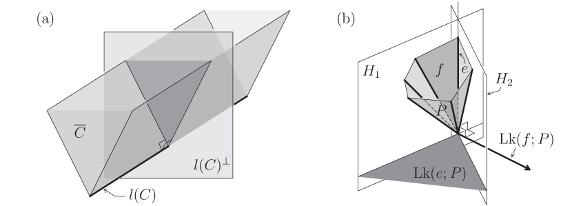
Figure 2.1: (a) Illustration of Lemma 2.1 (Decomposition Theorem). (b) Links $\textup{Lk}(e;P)$ and $\textup{Lk}(f;P)$ in a polytopal cone $P$.

If $f$ has dimension $m$ then $L(f)$ is $m$-dimensional and $L(f)^{\bot}$ is $(n-m)$-dimensional. Because $P_{f}$ has full-dimension in $\mathbb{R}^{n}$, $P_{f}\cap L(f)^{\bot}$ is also full-dimensional in $L(f)^{\bot}$. It follows that the link $\textup{Lk}(f;P)$ is an $(n-m)$-dimensional polytopal cone in $L(f)^{\bot}\subset\mathbb{R}^{n}$ with its defining halfspaces being $H_{i}^{+}\cap L(f)^{\bot}$.

We defined the link $\textup{Lk}(f;P)$ under the assumption that $P$ is an $n$-dimensional polyhedron in $\mathbb{R}^{n}$. If $P$ is $n^{\prime}$-dimensional with $n^{\prime}<n$, however, we just consider the smallest linear subspace $L(P)$ containing $P$ and define the link $\textup{Lk}(f;P)$ with respect to $L(P)$ in the same manner as above. Thus if $f$ is $m$-dimensional, its link $\textup{Lk}(f;P)$ is an $(n^{\prime}-m)$-dimensional polytopal cone in $L(P)\cap L(f)^{\bot}\subset\mathbb{R}^{n}$.

Let $P$ be an $n$-dimensional polyhedral cone in $\mathbb{R}^{n}$. Let $f$ be a face of $P$ and $e$ a face of $f$. We define a subset $f_{(e;P)}$ of the link $\textup{Lk}(e;P)$ as:

$$f_{(e;P)}=\textup{Lk}(e;P)\cap L(f).$$

The lemma below says that $f_{(e;P)}$ is a face of the polytopal cone $\textup{Lk}(e;P)$, whose link in $\textup{Lk}(e;P)$ is equal to the link $\textup{Lk}(f;P)$. Thus the link $\textup{Lk}(e;P)$ of $e$ has all the information about the links $\textup{Lk}(f;P)$ of those faces $f$ which contain $e$; this fact enables us to use inductive arguments on links later on.

Lemma 2.3.

Let $P$ be an $n$-dimensional polyhedral cone in $\mathbb{R}^{n}$. Let $f$ be a face of $P$ and $e$ a face of $f$. Then $f_{(e;P)}$ is a face of the polytopal cone $\textup{Lk}(e;P)$. If $f$ is a facet of $P$ then $f_{(e;P)}$ is also a facet of $\textup{Lk}(e;P)$. Furthermore, we have the following identity between the two links involved:

$$\textup{Lk}(f;P)=\textup{Lk}[f_{(e;P)};\textup{Lk}(e;P)].$$

Proof.

We write $P=\bigcap_{i=1}^{m}H_{i}^{+}$ for an irredundant family $\{H_{i}^{+}\}$ of halfspaces of $\mathbb{R}^{n}$ bounded by $H_{i}$. We may assume that for some $m_{f}<m_{e}<m$ the faces $f$ and $e$ are expressed as

$$f =P\cap(H_{1}\cap\cdots\cap H_{m_{f}})$$

$$e =P\cap(H_{1}\cap\cdots\cap H_{m_{f}}\cap H_{m_{f}+1}\cap\cdots\cap H_{m_{e}}).$$

If we set, as before,

$$P_{f} =H_{1}^{+}\cap\cdots\cap H_{m_{f}}^{+}$$

$$P_{e} =H_{1}^{+}\cap\cdots\cap H_{m_{f}}^{+}\cap H_{m_{f}+1}^{+}\cap\cdots\cap H_{m_{e}}^{+},$$

then the links of $f$ and $e$ are by definition

$$\textup{Lk}(f;P) =P_{f}\cap L(f)^{\bot}$$

$$\textup{Lk}(e;P) =P_{e}\cap L(e)^{\bot}=\bigcap_{i=1}^{m_{e}}(H_{i}^{+}\cap L(e)^{\bot}).$$

Because $L(f)=H_{1}\cap\cdots\cap H_{m_{f}}$ and $\textup{Lk}(e;P)\subset L(e)^{\bot}$, we then have

$$f_{(e;P)} =\textup{Lk}(e;P)\cap L(f)$$

$$=\textup{Lk}(e;P)\cap(H_{1}\cap\cdots\cap H_{m_{f}})$$

$$=\textup{Lk}(e;P)\cap[(H_{1}\cap L(e)^{\bot})\cap\cdots\cap(H_{m_{f}}\cap L(e)^{\bot})].$$

Since $m_{f}<m_{e}$ and the defining halfspaces of $\textup{Lk}(e;P)$ are $H_{i}^{+}\cap L(e)^{\bot}$ $(1\leq i\leq m_{e})$, this shows that $f_{(e;P)}$ is a face of the polytopal cone $\textup{Lk}(e;P)$. If $f$ is a facet of $P$ then $m_{f}=1$ and $f=P\cap H_{1}$. Therefore, $f_{(e;P)}=\textup{Lk}(e;P)\cap(H_{1}\cap L(e)^{\bot})$ is a facet of $\textup{Lk}(e;P)$.

To see the claimed equality we first note that, because $\textup{Lk}(e;P)\subset L(e)^{\bot}$ has non-empty interior in $L(e)^{\bot}$,

$$L(f_{(e;P)})=L[\textup{Lk}(e;P)\cap L(f)]=L(e)^{\bot}\cap L(f).$$

Because $e\subset f$ and hence $L(e)\subset L(f)$, we then have

$$L(e)^{\bot}\cap L(f_{(e;P)})^{\bot}=L(e)^{\bot}\cap(L(e)+L(f)^{\bot})=L(f)^{\bot}.$$

Finally, unraveling all the definitions, we see that

$$\textup{Lk}[f_{(e;P)};\textup{Lk}(e;P)] =\textup{Lk}(e;P)_{f_{(e;P)}}\cap L(f_{(e;P)})^{\bot}$$

$$=[(H_{1}^{+}\cap L(e)^{\bot})\cap\cdots\cap(H_{m_{f}}^{+}\cap L(e)^{\bot})]\cap L(f_{(e;P)})^{\bot}$$

$$=(H_{1}^{+}\cap\cdots\cap H_{m_{f}}^{+})\cap L(e)^{\bot}\cap L(f_{(e;P)})^{\bot}$$

$$=P_{f}\cap L(f)^{\bot}$$

$$=\textup{Lk}(f;P).\qed$$

2.4 Spherical polytopes

Let $\mathbb{S}^{n}$ be the unit sphere in $\mathbb{R}^{n+1}$. To any subset $S\subset\mathbb{S}^{n}$ we associate the cone $\mathsf{\Lambda}_{S}$ over $S$ defined by

$$\mathsf{\Lambda}_{S}=\{ax\in\mathbb{R}^{n+1}\,|\,x\in S,a\geq 0\}.$$

For a subset $S\subset\mathbb{S}^{n}$ and a cone $C\subset\mathbb{R}^{n+1}$, it is clear that

$$\mathsf{\Lambda}_{S}\cap\mathbb{S}^{n}=S\;\;\text{and}\;\;\mathsf{\Lambda}_{C\cap\mathbb{S}^{n}}=C\cup\{o\}.$$

A subset $L\subset\mathbb{S}^{n}$ is an $m$-plane provided that the cone $\mathsf{\Lambda}_{L}$ over $L$ is an $(m+1)$-dimensional linear subspace of $\mathbb{R}^{n+1}$. The orthogonal complement $L^{\bot}$ of an $m$-plane $L$ is defined to be $(\mathsf{\Lambda}_{L})^{\bot}\cap\mathbb{S}^{n}$.

Let $S$ be a subset of $\mathbb{S}^{n}$. The smallest $m$-plane containing $S$ is denoted $L(S)$ and is clearly equal to $L(\mathsf{\Lambda}_{S})\cap\mathbb{S}^{n}$. The dimension of $S$ is defined to be the dimension of this plane. We call $S$ open if it is open relative to $L(S)$. Likewise, a point $x\in S$ is called an interior (resp. boundary) point of $S$ if $x$ is an interior (resp. boundary) point of $S$ relative to $L(S)$. We also denote by $S^{\circ}$ the set of interior points of $S$.

A subset $S\subset\mathbb{S}^{n}$ is convex (resp. properly convex) if the cone $\mathsf{\Lambda}_{S}$ over $S$ is a convex cone (resp. line-free convex cone). It is clear that $S\subset\mathbb{S}^{n}$ is convex if and only if for any two points in $S$ the (spherical) geodesic connecting them is in $S$. A subset $S\subset\mathbb{S}^{n}$ is locally convex if every point of $S$ has a neighborhood in $S$ which is a convex subset of $\mathbb{S}^{n}$. The convex hull $\textup{conv}(S)$ of a subset $S$ is the smallest convex subset containing $S$. Finally, a subset $S\subset\mathbb{S}^{n}$ is a noun if the cone $\mathsf{\Lambda}_{S}$ over $S$ is a noun in $\mathbb{R}^{n+1}$, where the noun stands for hyperplane, halfspace, support or face. Note that if $S\neq\mathbb{S}^{n}$ is convex then $\mathsf{\Lambda}_{S}\neq\mathbb{R}^{n+1}$ is a convex cone and is contained in a halfspace of $\mathbb{R}^{n+1}$. Thus every convex subset $S$ not equal to $\mathbb{S}^{n}$ is contained in a halfspace of $\mathbb{S}^{n}$ and hence has diameter at most $\pi$.

A subset $P\subset\mathbb{S}^{n}$ is a polyhedron (resp. polytope) if the cone $\mathsf{\Lambda}_{P}$ over $P$ is a polyhedral cone (resp. polytopal cone) in $\mathbb{R}^{n+1}$. If a polyhedron $P$ has dimension $m$ we call $P$ an $m$-polyhedron and similarly for polytopes. A maximal face of $P$ is called a facet of $P$. A ridge of $P$ is a facet of a facet of $P$. A vertex (resp. edge) of $P$ is a $0$-dimensional (resp. $1$-dimensional) face of $P$. Let $P=\bigcap_{i=1}^{m}H_{i}^{+}$ where the $H_{i}^{+}$ are halfspaces bounded by hyperplanes $H_{i}$, that is, $H_{i}^{+}=(\mathsf{\Lambda}_{H_{i}})^{+}\cap\mathbb{S}^{n}$. Under the same irredundancy condition on the family $\{H_{i}^{+}\}$ as in Section 2.2, the same properties of faces of $P$ as listed therein hold.

Let $P\subset\mathbb{S}^{n}$ be a polyhedron and $f$ a face of $P$. The link $\textup{Lk}(f;P)$ of $f$ in $P$ is by definition

$$\textup{Lk}(f;P)=\textup{Lk}(\mathsf{\Lambda}_{f};\mathsf{\Lambda}_{P})\cap\mathbb{S}^{n}.$$

See Figure 2.2.

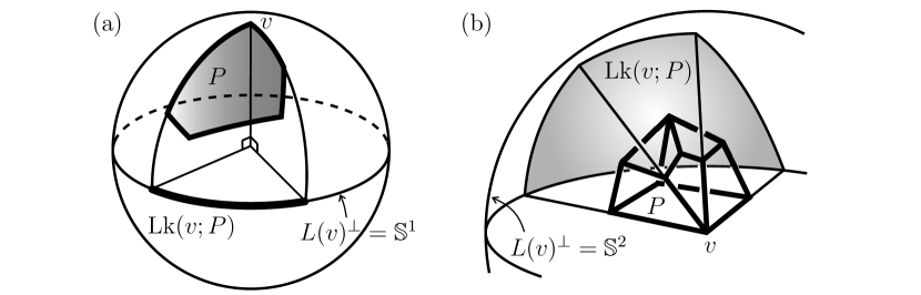
Figure 2.2: Links $\textup{Lk}(v;P)$ of $v$ in $P$ are drawn in (a) and (b). The ambient space of (b) is $\mathbb{S}^{3}$.

Because $\textup{Lk}(\mathsf{\Lambda}_{f};\mathsf{\Lambda}_{P})$ is a polytopal cone, the link $\textup{Lk}(f;P)$ is a polytope in $\mathbb{S}^{n}$. If $P$ is an $n$-polyhedron and $f$ is an $m$-face then the link $\textup{Lk}(f;P)$ is an $(n-m-1)$-polytope. Let $e$ be a face of $f$ and define a subset $f_{(e;P)}$ of $\textup{Lk}(e;P)$ by

$$f_{(e;P)}=\textup{Lk}(e;P)\cap L(f).$$

It then follows from Lemma 2.3 that $f_{(e;P)}$ is a face of the polytope $\textup{Lk}(e;P)$ and the following identity holds between the two links involved:

$$\textup{Lk}(f;P)=\textup{Lk}(f_{(e;P)};\textup{Lk}(e;P)).$$ (2.4.1)

2.5 Duality

Let $\mathbb{R}_{n}$ be the dual vector space $(\mathbb{R}^{n})^{*}=\textup{Hom}(\mathbb{R}^{n},\mathbb{R})$ of $\mathbb{R}^{n}$. It is equipped with the standard inner product coming from that of $\mathbb{R}^{n}$. Denote by $\mathbb{S}_{n}$ the unit sphere in $\mathbb{R}_{n}$.

Let $C$ be a cone in $\mathbb{R}^{n}$. The dual cone $C^{*}$ of $C$ is defined by

$$C^{*}=\{u\in\mathbb{R}_{n}\,|\,u(x)\leq 0\;\text{for all}\;x\in C\}.$$

It is easy to see that $C^{*}$ is a closed convex cone in $\mathbb{R}_{n}$. If $L$ is an $m$-dimensional linear subspace of $\mathbb{R}^{n}$ then $L^{*}$ is an $(n-m)$-dimensional linear subspace of $\mathbb{R}_{n}$. If $H^{+}$ is a halfspace bounded by a hyperplane $H$ then $(H^{+})^{*}$ is a ray in $\mathbb{R}_{n}$. We have the following well-known facts (compare with [8] and [6]):

• If $C$ is a closed convex cone then $C^{**}=C$ (under the natural identification $(\mathbb{R}_{n})^{*}=\mathbb{R}^{n}$) and

  $$\dim L(C^{*})+\dim l(C) =n;$$

  $$\dim L(C)+\dim l(C^{*}) =n.$$

• If $C$ and $D$ are closed convex cones then

  $$(C\cap D)^{*}=\textup{conv}(C^{*}\cup D^{*}).$$

• If $P$ is a polyhedral cone then so too is $P^{*}$.

• If $P$ is an $n$-dimensional polytopal cone then so too is $P^{*}$.

Let $S$ be a subset of $\mathbb{S}^{n}$. The dual $S^{*}$ of $S$ is defined by

$$S^{*}=(\mathsf{\Lambda}_{S})^{*}\cap\mathbb{S}_{n}.$$

Thus the dual $S^{*}$ of $S$ is always a closed convex subset of $\mathbb{S}_{n}$. If $L\subset\mathbb{S}^{n}$ is an $m$-plane then $L^{*}$ is an $(n-m-1)$-plane. In particular, the dual of a hyperplane $H$ is a pair $\{\pm v\}=\mathbb{S}_{0}$ of antipodal points. The dual of a halfspace is a single point; if $(H^{+})^{*}=v$ then $(H^{-})^{*}=-v$. The analogous properties for cones as listed above also hold for subsets of $\mathbb{S}^{n}$. In particular, if $P\subset\mathbb{S}^{n}$ is an $n$-polytope then so too is its dual $P^{*}$; if $P$ is expressed as

$$P=\bigcap_{i=1}^{m}H_{i}^{+},$$

then

$$P^{*}=\left[\bigcap_{i=1}^{m}H_{i}^{+}\right]^{*}=\textup{conv}\left[\bigcup_{i=1}^{m}(H_{i}^{+})^{*}\right]=\textup{conv}\{v_{1},v_{1},\ldots,v_{m}\},$$

where each $v_{i}=(H_{i}^{+})^{*}$ becomes a vertex of the dual polytope $P^{*}$.

2.6 Alexandrov spaces of curvature bounded below

The main reference for this subsection is [4]. Fix a real number $\kappa$. Let $M_{\kappa}^{n}$ be the $n$-dimensional complete simply-connected Riemannian manifold of constant curvature $\kappa$, and denote $D_{\kappa}=\pi/\sqrt{\kappa}$ for $\kappa>0$ and $D_{\kappa}=\infty$ for $\kappa\leq 0$. Thus, for example, we have $M_{1}^{n}=\mathbb{S}^{n}$ and $D_{1}=\pi$. We denote by $d$ the induced path metric on $M_{\kappa}^{n}$.

Let $X$ be a metric space. Given three points $p,q,r\in X$ satisfying

$$d(p,q)+d(q,r)+d(r,p)<2D_{\kappa},$$

there is a comparison triangle $\triangle(\bar{p},\bar{q},\bar{r})$ in $M_{\kappa}^{2}$, namely, three points $\bar{p},\bar{q},\bar{r}\in M_{\kappa}^{2}$ such that

$$d(\bar{p},\bar{q})=d(p,q),\;\;d(\bar{q},\bar{r})=d(q,r),\;\;d(\bar{r},\bar{p})=d(r,p).$$

We define $\bar{\angle}pqr$ to be the angle at the vertex $\bar{q}$ of the triangle $\triangle(\bar{p},\bar{q},\bar{r})$.

Let $X$ be a path metric space, that is, a metric space where the distance $d$ between each pair of points is equal to the infimum of the length of rectifiable curves joining them. Then $X$ is said to be $\textup{Alex}(\kappa)$ provided that for any four distinct points $b,c,d$ and $a$ in $X$ we have the inequality

$$\bar{\angle}bac+\bar{\angle}cad+\bar{\angle}dab\leq 2\pi.$$

(If $X$ is a $1$-dimensional manifold and $\kappa>0$, then we require in addition that its diameter be at most $D_{\kappa}$.) The path metric space $X$ is said to be locally $\textup{Alex}(\kappa)$, or more commonly, an Alexandrov space of curvature $\geq\kappa$, if each point $x\in X$ has a neighborhood $U_{x}$ which is $\textup{Alex}(\kappa)$.

Examples of locally $\textup{Alex}(\kappa)$ spaces include Riemannian manifolds without boundary or with locally convex boundary whose sectional curvatures are $\geq\kappa$. (Locally) convex subsets of such Riemannian manifolds are also locally $\textup{Alex}(\kappa)$. We shall be interested mostly in the case when $\kappa=1$ and $M_{1}^{n}=\mathbb{S}^{n}$ – locally convex subsets of $\mathbb{S}^{n}$ are locally $\textup{Alex}(1)$.

The following is a local-to-global theorem for $\textup{Alex}(\kappa)$ spaces which is analogous to the Cartan-Hadamard theorem for $\textup{CAT}(\kappa)$ spaces with $\kappa\leq 0$ (see for example [3]). Unlike the Cartan-Hadamard theorem, however, we do not place any topological restriction on the space in this theorem:

Theorem 2.4 (Globalization Theorem).

If a complete path metric space is locally $\textup{Alex}(\kappa)$, then it is $\textup{Alex}(\kappa)$ and has diameter $\leq D_{\kappa}$.

For its proof we refer to [4]. As a corollary of the globalization theorem, we have the following criterion for locally convex subsets of $M_{\kappa}^{n}$ to be convex. Note that if $\kappa>0$, geodesics in $M_{\kappa}^{n}$ have length at most $D_{\kappa}$.

Corollary 2.5.

Let $C$ be a locally convex connected subset of $M_{\kappa}^{n}$. If $\kappa>0$, we assume in addition that $C$ is not a $1$-dimensional manifold. If $C$ is complete and locally compact with respect to the induced path metric, then $C$ is convex in $M_{\kappa}^{n}$.

Proof.

Because $C$ is locally convex in $M_{\kappa}^{n}$ (and is not a $1$-dimensional manifold in case $\kappa>0$), $C$ is locally $\textup{Alex}(\kappa)$. If $C$ is complete with respect to the induced length metric, the globalization theorem tells us that $C$ is an $\textup{Alex}(\kappa)$ space of diameter $\leq D_{\kappa}$. Let $p$ and $q$ be two points of $C$. Because $C$ is connected, complete and locally compact with respect to the induced path metric, $C$ satisfies the assumption of the Hopf-Rinow Theorem (see for example [3]) and hence there is a geodesic $[p,q]_{C}$ in $C$ joining $p$ and $q$. As $C$ is locally convex, however, this curve $[p,q]_{C}$ has to be a local geodesic in $M_{\kappa}^{n}$. Since $C$ has diameter $\leq D_{\kappa}$, the length of $[p,q]_{C}$ is at most $D_{\kappa}$. It follows from the simple-connectedness of $M_{\kappa}^{n}$ that $[p,q]_{C}$ is a (global) geodesic in $M_{\kappa}^{n}$. ∎

3 Main objects

We define metric polyhedral complexes which are locally isometric to $\mathbb{S}^{n}$. Our presentation follows that of $M_{\kappa}$–polyhedral complexes in [3], where $\kappa=1$ in our case. We consider subcomplexes of such polyhedral complexes that embed isometrically into $\mathbb{S}^{n}$ as topological balls, and present a convexity criterion for them. We also study special subcomplexes called stars and residues.

3.1 Complexes

Definition 3.1 ($n$-complexes).

Given a family $\{P_{i}:i\in\mathcal{I}\}$ of $n$-polytopes in $\mathbb{S}^{n}$, let $X$ be a connected $n$-manifold (possibly with non-empty boundary $\partial X$) which is obtained by gluing together members of $\{P_{i}\}$ along their respective facets by isometries. We denote by $\sim$ the equivalence relation on the disjoint union $\bigsqcup_{i\in\mathcal{I}}P_{i}$ induced by this gluing so that

$$X={\bigsqcup_{i\in\mathcal{I}}P_{i}}/\sim.$$

Let $\pi:\bigsqcup_{i\in\mathcal{I}}P_{i}\to X$ be the natural projection and denote $\pi_{i}=\pi|_{P_{i}}$. We call the manifold $X$ a spherical polytopal $n$-complex ($n$-complex, for short) provided that

1. the family $\{\pi_{i}(P_{i})\,|\,i\in\mathcal{I}\}$ is locally finite;

2. it is endowed with the quotient metric associated to the projection $\pi$;

3. its interior $X^{\circ}$ is locally isometric to $\mathbb{S}^{n}$;

4. it is simply-connected.

For each $n$-complex $X$ the conditions (3) and (4) guarantee that there is an associated developing map

$$dev:X\to\mathbb{S}^{n}$$

which is a local isometry on the interior of $X$ and which extends naturally to the boundary of $X$. The developing map is well-defined up to post-composition with an isometry of $\mathbb{S}^{n}$.

Convention 3.2.

Whenever we mention an $n$-complex $X$, we shall tacitly assume that a developing map $dev:X\to\mathbb{S}^{n}$ for $X$ is already chosen. Given a subset $K\subset X$, we shall denote by $K_{\mathbb{S}}$ the image $dev(K)$ of $K$ under this developing map $dev$.

Let $X$ be an $n$-complex. A subset $f\subset X$ is called an $m$-cell if it is the image $\pi_{i}(f_{i})$ for some $m$-face $f_{i}$ of $P_{i}$; the interior of $f$ is the image under $\pi_{i}$ of the interior of $f_{i}$. The $0$-cells, $1$-cells, $(n-2)$-cells and $(n-1)$-cells of $X$ are also called vertices, edges, ridges and facets of $X$, respectively. Two $m$-cells $f_{1}$ and $f_{2}$ of $X$ are said to be adjacent if their intersection $f_{1}\cap f_{2}$ is an $(m-1)$-cell of $X$. A subcomplex of $X$ is a union of cells of $X$.

3.2 Links in complexes

Let $X$ be an $n$-complex. For each $m$-cell $e$ of $X$ with $m<n$, we denote $\mathcal{I}(e)=\{i\in\mathcal{I}\,|\,e\subset\pi_{i}(P_{i})\}$. The link $\textup{Lk}(e;X)$ of $e$ in $X$ is an $(n-m-1)$-complex defined as follows.

Let $\sigma$ be a facet of $X$ containing $e$ and let $\mathcal{I}(\sigma)=\{j,k\}\subset\mathcal{I}(e)$. For each $i\in\mathcal{I}(\sigma)$ let $e_{i}$ and $\sigma_{i}$ be faces of $P_{i}$ such that $\pi_{i}(e_{i})=e$ and $\pi_{i}(\sigma_{i})=\sigma$. By definition of $n$-complex, the facets $\sigma_{j}$ and $\sigma_{k}$ are isometric by an isometry $\phi_{jk}$ which restricts to an isometry between $e_{j}$ and $e_{k}$. Then $\phi_{jk}$ induces an isometry between $(\sigma_{j})_{(e_{j};P_{j})}$ and $(\sigma_{k})_{(e_{k};P_{k})}$. Because $(\sigma_{i})_{(e_{i};P_{i})}$ is a facet of the polytope $\textup{Lk}(e_{i};P_{i})$ for each $i\in\mathcal{I}(\sigma)$, this shows that the equivalence relation $\sim$ on $\bigsqcup_{i\in\mathcal{I}}P_{i}$ induces an equivalence relation $\sim_{\sigma}$ on $\textup{Lk}(e_{j};P_{j})\bigsqcup\textup{Lk}(e_{k};P_{k})$. Combining all equivalence relations $\sim_{\sigma}$ for all facets $\sigma$ of $X$ containing $e$, we obtain an equivalence relation $\sim_{e}$ on $\bigsqcup_{i\in\mathcal{I}(e)}\textup{Lk}(e_{i};P_{i})$. The link $\textup{Lk}(e;X)$ of $e$ in $X$ is then defined as

$$\textup{Lk}(e;X)=\bigsqcup_{i\in\mathcal{I}(e)}\textup{Lk}(e_{i};P_{i})/\sim_{e}$$

and is an $(n-m-1)$-complex endowed with the quotient metric associated to the natural projection $\bigsqcup_{i\in\mathcal{I}(e)}\textup{Lk}(e_{i};P_{i})\to\textup{Lk}(e;X)$ induced by $\sim_{e}$. Indeed, because $X$ is a manifold, if $e$ is contained in the boundary of $X$ then the link $\textup{Lk}(e;X)$ is isometric to a ball in $\mathbb{S}^{n-m-1}$; otherwise, it is isometric to the sphere $\mathbb{S}^{n-m-1}$. Thus it is simply-connected and its interior is locally isometric to the sphere $\mathbb{S}^{n-m-1}$.

Let $X$ be an $n$-complex. We can extend the identity (2.4.1) (which is obtained from Lemma 2.3) to the current setting as follows. Let $e\subsetneq f$ be cells of $X$. Keeping the same notation as above, we recall that the link $\textup{Lk}(e;X)$ is the quotient of $\bigsqcup_{i\in\mathcal{I}(e)}\textup{Lk}(e_{i};P_{i})$ by $\sim_{e}$, where $e_{i}$ is a face of $P_{i}$ such that $\pi_{i}(e_{i})=e$ for each $i\in\mathcal{I}(e)$. Consider $\mathcal{I}(f)=\{i\in\mathcal{I}\,|\,f\subset\pi_{i}(P_{i})\}\subset\mathcal{I}(e)$. For each $i\in\mathcal{I}(f)$ let $f_{i}$ be the face of $P_{i}$ such that $\pi_{i}(f_{i})=f$. Now by Lemma 2.3 we have that $(f_{i})_{(e_{i};P_{i})}$ is a face of $\textup{Lk}(e_{i};P_{i})$ for each $i\in\mathcal{I}(f)$. Since $\sim_{e}$ identifies all $(f_{i})_{(e_{i};P_{i})}$ for $i\in\mathcal{I}(f)$, we may define

$$f_{(e;X)}=\pi_{i}({f_{i}}_{(e_{i};P_{i})})$$ (3.2.1)

for any chosen $i\in\mathcal{I}(f)$ and it follows that $f_{(e;X)}$ is a cell of the complex $\textup{Lk}(e;X)$. From the identity (2.4.1) we see that the equivalence relation $\sim_{f_{(e;X)}}$ on $\bigsqcup_{i\in\mathcal{I}(f)}\textup{Lk}({f_{i}}_{(e_{i};P_{i})};\textup{Lk}(e_{i};P_{i}))$, which is by definition induced from $\sim_{e}$, is equal to the equivalence relation $\sim_{f}$ on $\bigsqcup_{i\in\mathcal{I}(f)}\textup{Lk}(f_{i};P_{i})$. It now follows that

$$\textup{Lk}(f;X) =\bigsqcup_{i\in\mathcal{I}(f)}\textup{Lk}(f_{i};P_{i})/\sim_{f}$$

$$=\bigsqcup_{i\in\mathcal{I}(f)}\textup{Lk}({f_{i}}_{(e_{i};P_{i})};\textup{Lk}(e_{i};P_{i}))/\sim_{f_{(e;X)}}$$

$$=\textup{Lk}(f_{(e;X)};\textup{Lk}(e;X)).$$ (3.2.2)

3.3 Polyballs

Recall that an $n$-complex is equipped with a developing map into $\mathbb{S}^{n}$.

Definition 3.3 (Polyballs).

An $n$-polyball $B$ is an $n$-complex which is topologically an $n$-dimensional ball with boundary and whose developing map

$$dev:B\hookrightarrow\mathbb{S}^{n}$$

is an isometric embedding into $\mathbb{S}^{n}$. An $n$-polyball $B$ is said to be convex (resp. locally convex) if its developing image $B_{\mathbb{S}}=dev(B)$ is a convex (resp. locally convex) subset of $\mathbb{S}^{n}$.

Being compact, an $n$-polyball consists of a finite number of $n$-cells. In particular, a single $n$-cell is itself an $n$-polyball. If $X$ is an $n$-complex with boundary and $f$ is an $m$-cell in the boundary of $X$, then the link $\textup{Lk}(f;X)$ is an $(n-m-1)$-polyball.

Let $B$ be a fixed $n$-polyball from now on. Because $B$ consists of a finite number of $n$-cells $P$ and because their images $P_{\mathbb{S}}$ are compact convex subsets of $\mathbb{S}^{n}$, its image $B_{\mathbb{S}}$ in $\mathbb{S}^{n}$ is compact with respect to the path metric induced from that of the sphere $\mathbb{S}^{n}$. Thus if we know that $B$ is locally convex, then it follows from Corollary 2.5 (applied to $M_{1}^{n}=\mathbb{S}^{n}$) that $B$ is convex. See Lemma 3.4 below. Therefore, to establish convexity of $B$, it suffices to investigate local convexity of $B$.

Because the $n$-polyball $B$ is a manifold, its local convexity matters only at its boundary points. Because of the polyhedral structure of $B$, however, it suffices to investigate the links of cells in the boundary of $B$. More precisely, let $x$ be a point in the boundary of $B$. There is a unique cell $f$ of $B$ that contains $x$ as its interior point. The local geometry of $B$ at $x$ is completely determined by the union of $n$-cells containing $f$, whose geometry is then captured by the link of $f$ in $B$. Thus $B_{\mathbb{S}}$ is locally convex at $x_{\mathbb{S}}$ if and only if the link $\textup{Lk}(f;B)$ is a convex polyball. Therefore, $B$ is locally convex if and only if the links $\textup{Lk}(f;B)$ are convex polyballs for all cells $f$ in the boundary of $B$. This last condition holds for facets $\sigma$ in the boundary of $B$ since the link $\textup{Lk}(\sigma;B)$ is just a singleton of $\mathbb{S}^{0}$ and hence convex. Thus we are left with cells of dimension at most $n-2$. It turns out that only $(n-2)$-cells, i.e. the ridges of $B$, need to be investigated.

Let $f$ be an $m$-cell in the boundary of $B$. The link $\textup{Lk}(f;B)$ of $f$ is an $(n-m-1)$-polyball. On the other hand, if $v$ is a vertex of $f$, then $f$ descends to an $(m-1)$-cell $f_{(v;B)}$ in the link $\textup{Lk}(v;B)$ of $v$. The link $\textup{Lk}(v;B)$ is an $(n-1)$-polyball with $f_{(v;B)}$ in its boundary. From (3.2) of the previous subsection, we have the following identity between the two $(n-m-1)$-polyballs

$$\textup{Lk}(f;B)=\textup{Lk}(f_{(v;B)};\textup{Lk}(v;B)).$$ (3.3.1)

Therefore, the link $\textup{Lk}(v;B)$ of the vertex $v$ contains all the information about the links $\textup{Lk}(f;B)$ of those cells $f$ which contain $v$. In particular, if the link $\textup{Lk}(v;B)$ of $v$ is a convex $(n-1)$-polyball then the link $\textup{Lk}(f;B)$ of $f$ is also a convex $(n-m-1)$-polyball.

Conversely, the proof of the lemma below shows that if the links $\textup{Lk}(e;B)$ are convex for all ridges $e$ of $B$ in the boundary of $B$, then $\textup{Lk}(v;B)$ is convex for every boundary vertex $v$.

Lemma 3.4.

Let $B$ be an $n$-polyball. If the links $\textup{Lk}(e;B)$ are convex for all ridges $e$ contained in the boundary of $B$, then $B$ is convex.

Proof.

We shall prove the lemma by induction on the dimension $n$ of $B$. In the base case when $n=2$, the ridges of $B$ are just vertices of $B$. From the above discussion we see that $B$ is locally convex. By Corollary 2.5, $B$ is convex.

Suppose now that the assertion is true for polyballs of dimension $\leq n-1$. Let $B$ be an $n$-polyball and assume that the links $\textup{Lk}(e;B)$ are convex for all ridges $e$ contained in the boundary of $B$. Let $v$ be a vertex in the boundary of $B$. Then the link $\textup{Lk}(v;B)$ is an $(n-1)$-polyball and its ridges are those $e_{(v;B)}$ which come from the ridges $e$ of $B$ that contain $v$. The ridges $e_{(v;B)}$ are in the boundary of $\textup{Lk}(v;B)$ if and only if the ridges $e$ are in the boundary of $B$. Because $\textup{Lk}(e;B)$ is assumed to be convex, it follows from (3.3.1) that $\textup{Lk}(e_{(v;B)};\textup{Lk}(v;B))$ is convex, too. Hence the induction hypothesis applies and we conclude that $\textup{Lk}(v;B)$ is convex. Since $v$ is arbitrary, this implies that $B$ is locally convex. By Corollary 2.5 once again, we conclude that $B$ is convex. The induction steps are complete. ∎

3.4 Stars and residues

Let $X={\bigsqcup_{i\in I}P_{i}}/\sim$ be a fixed $n$-complex throughout this subsection. We shall define two kinds of subcomplexes of $X$ called stars and residues. In most cases later on they will be $n$-polyballs in their own right.

Definition 3.5 (Stars and residues).

Let $Y\subset X$ be a subcomplex and let $\sigma\subset Y$ be a cell or a subcomplex of $X$.

1. The star $st(\sigma;Y)$ of $\sigma$ in $Y$ is the union of the cells of $Y$ that intersect $\sigma$.

2. The residue $res(\sigma;Y)$ of $\sigma$ in $Y$ is the union of the cells of $Y$ which contain $\sigma$.

We set $st^{0}(\sigma;Y)=\sigma$ and define $st^{k+1}(\sigma;Y)=st(st^{k}(\sigma;Y);Y)$ inductively. In case $Y=X$ we simply denote $st^{k}(\sigma)=st^{k}(\sigma;X)$ and $res(\sigma)=res(\sigma;X)$. Notice that $st(v)=res(v)$ for vertices $v$ of $X$.

Let $Y_{1}$ and $Y_{2}$ be subcomplexes of $X$. The following relations are immediate from the definition of star.

$$st(Y_{1}\cup Y_{2})=st(Y_{1})\cup st(Y_{2});$$ (3.4.1)

$$st(Y_{1}\cap Y_{2})\subset st(Y_{1})\cap st(Y_{2}).$$ (3.4.2)

Iterated stars satisfy the following properties. Let $P_{0}$ be an $n$-cell in $X$ and let $\mathcal{V}$ be the set of all vertices in $P_{0}$. It follows directly from the definition that

$$P_{0}=\bigcap_{v\in\mathcal{V}}st(v)\quad\text{and}\quad st(P_{0})=\bigcup_{v\in\mathcal{V}}st(v).$$ (3.4.3)

Let $\mathcal{P}$ be the set of all $n$-cells in $st(P_{0})$. We claim that for each $k\geq 1$

$$P_{0}\subset\bigcap_{P\in\mathcal{P}}st^{k}(P)\quad\text{and}\quad st^{k+1}(P_{0})=\bigcup_{P\in\mathcal{P}}st^{k}(P).$$ (3.4.4)

The former inclusion is obvious. We can see the latter equality using induction on $k$. The base case $k=1$ follows immediately from the definition. Suppose it is true up to $k-1$. We then have $st^{k+1}(P_{0})=st(st^{k}(P_{0}))=st(\bigcup_{\mathcal{P}}st^{k-1}(P))=\bigcup_{\mathcal{P}}st(st^{k-1}(P))=\bigcup_{\mathcal{P}}st^{k}(P)$, where the third equality follows from (3.4.1). See Figure 3.1 (a). Using properties (3.4.3) and (3.4.4) we can prove the following lemma.

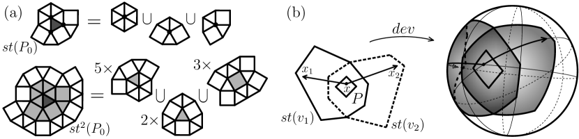
Figure 3.1: (a) Illustrations of (3.4.3) and (3.4.4). (b) Proof of Lemma 3.6.

Lemma 3.6.

Let $X$ be an $n$-complex.

1. If $st(v)$ is a convex $n$-polyball for all vertices $v$ of $X$, then $st(P)$ is an $n$-polyball for each $n$-cell $P$ in $X$.

2. For each fixed $k\geq 1$, if $st^{k}(P)$ is a convex $n$-polyball for all $n$-cells $P$ in $X$, then $st^{k+1}(P)$ is an $n$-polyball.

Proof.

Recall that we have a developing map $dev:X\to\mathbb{S}^{n}$ of the $n$-complex $X$ and we denote $K_{\mathbb{S}}=dev(K)$ for $K\subset X$.

(1) Let $P$ be an $n$-cell of $X$. Let $x_{1},x_{2}\in st(P)$ be such that $x_{1}\neq x_{2}$. We want to show that $(x_{1})_{\mathbb{S}}\neq(x_{2})_{\mathbb{S}}$. Let $\mathcal{V}$ be the set of all vertices in $P$. The second identity of (3.4.3) implies that there are vertices $v_{1},v_{2}\in\mathcal{V}$ such that $x_{1}\in st(v_{1})$ and $x_{2}\in st(v_{2})$. If $x_{1},x_{2}\in st(v_{1})\cap st(v_{2})$ then $(x_{1})_{\mathbb{S}}\neq(x_{2})_{\mathbb{S}}$, because $st(v_{1})\cap st(v_{2})\subset st(v_{1})$ and $st(v_{1})$ is a polyball and hence $dev|_{st(v_{1})}$ is an embedding. Thus we may assume from now on that $x_{1}\in st(v_{1})\setminus st(v_{2})$ and $x_{2}\in st(v_{2})\setminus st(v_{1})$. See Figure 3.1 (b).

Fix $i=1,2$. Consider the interior $P^{\circ}$ of $P$ and choose a point $x\in P^{\circ}$. Consider the geodesic segment $[(x)_{\mathbb{S}},(x_{i})_{\mathbb{S}}]$ in $\mathbb{S}^{n}$. Because $st(v_{i})$ is a convex polyball and because $(x)_{\mathbb{S}}\in(P^{\circ})_{\mathbb{S}}\subset st(v_{i})_{\mathbb{S}}$ by the first identity of (3.4.3), we must have that

$$[(x)_{\mathbb{S}},(x_{i})_{\mathbb{S}}]\subset st(v_{i})_{\mathbb{S}}.$$

Furthermore, the length of $[(x)_{\mathbb{S}},(x_{i})_{\mathbb{S}}]$ is less than $\pi$, since the diameter of the convex (proper) subset $st(v_{i})_{\mathbb{S}}$ is at most $\pi$ and $(x)_{\mathbb{S}}$ is an interior point of $st(v_{i})_{\mathbb{S}}$.

If the initial directions at $(x)_{\mathbb{S}}$ of $[(x)_{\mathbb{S}},(x_{1})_{\mathbb{S}}]$ and $[(x)_{\mathbb{S}},(x_{2})_{\mathbb{S}}]$ coincide, say,

$$[(x)_{\mathbb{S}},(x_{1})_{\mathbb{S}}]\subset[(x)_{\mathbb{S}},(x_{2})_{\mathbb{S}}]\subset st(v_{2})_{\mathbb{S}},$$

then we have $(x_{1})_{\mathbb{S}}\in st(v_{2})_{\mathbb{S}}$, contradictory to $x_{1}\in st(v_{1})\setminus st(v_{2})$. Thus the initial directions at $(x)_{\mathbb{S}}$ of the two geodesic segments must be different. Because their lengths are less than $\pi$, however, this implies that they intersect only at $(x)_{\mathbb{S}}$, hence $(x_{1})_{\mathbb{S}}\neq(x_{2})_{\mathbb{S}}$.

Thus we have shown that $dev$ is injective when restricted to the star $st(P)$. The identities in (3.4.3) again imply that $st(P)_{\mathbb{S}}$ is a union of convex subsets $st(v)_{\mathbb{S}}$ whose intersection has non-empty interior $(P^{\circ})_{\mathbb{S}}$. Therefore, the image $st(P)_{\mathbb{S}}$ is a topological ball, and this completes the proof that $st(P)$ is an $n$-polyball.

(2) For each fixed $k\geq 1$, the proof goes word-by-word in the same manner as in (1), except we need to use (3.4.4) instead. ∎

The residue of a cell $e$ serves as a nice neighborhood of the interior points of $e$. For example, let $B\subset X$ be a subcomplex which is an $n$-polyball. If $e$ is a cell in the boundary of $B$ and $x$ is an interior point of $e$, then $res(e;B)$ is a neighborhood of $x$ in $B$. Because the link of $e$ in $B$ depends only on the union of cells in $B$ that contain $e$, we have $\textup{Lk}(e;B)=\textup{Lk}(e;res(e;B))$. Therefore, once we know that $res(e;B)$ is a convex polyball, then we can conclude that $\textup{Lk}(e;B)$ is convex.

In view of Lemma 3.4, however, it is important for us to study the residues of ridges of $X$. So let $e$ be a ridge of $X$ and consider its residue $res(e)=res(e;X)$. Because ridges are $(n-2)$-dimensional, the link $\textup{Lk}(e,X)$ of $e$ is a $1$-complex embedded in $\mathbb{S}^{1}$ with its vertices and $1$-cells coming from $(n-1)$-cells and $n$-cells of $X$ containing $e$, respectively (see (3.2.1)). Indeed, the link $\textup{Lk}(e;X)$ is a circular arc or the whole $\mathbb{S}^{1}$ depending on whether $e$ is in the boundary of $X$ or not. Thus we can give a linear (or cyclic) order in the set of $n$-cells in $res(e)$ so that

$$res(e)=P_{1}\cup P_{2}\cup\cdots\cup P_{d_{e}},$$ (3.4.5)

where $P_{i}$ and $P_{i+1}$ are adjacent and share a common facet $\sigma_{i}=P_{i}\cap P_{i+1}$ (the indices are taken modulo $d_{e}$ in case $\textup{Lk}(e;X)=\mathbb{S}^{1}$) and $\sigma_{i}\cap\sigma_{j}=e$ for $i\neq j$.

We conclude this section with the following property of residues, which will lead to the definition of residual convexity in the next section. Let $0\leq m\leq n-1$. Let $f$ be an $(m+1)$-cell of $X$ and $\mathcal{H}$ be the set of all $m$-cells $h$ in $f$. We then have

$$res(f)=\bigcap_{h\in\mathcal{H}}res(h).$$ (3.4.6)

Indeed, the inclusion $res(f)\subset\bigcap_{h\in\mathcal{H}}res(h)$ is clear. If $\sigma\subset\bigcap_{h\in\mathcal{H}}res(h)$ is a cell, then $\sigma$ contains all $m$-cells in $f$. Thus $\sigma$ necessarily contains $f$ and hence $\sigma\subset res(f)$.

4 Convexity

This is the main section of the paper. Here we consider only those $n$-complexes $X$ which have empty boundary. We shall introduce local convexity conditions on $X$ called residual convexity and strong residual convexity. Combined with the global condition that $X$ is without boundary, these conditions enable us to show that $X$ is isometric to a convex proper domain in $\mathbb{S}^{n}$. We also provide a simple combinatorial condition for a residually convex complex to be strongly residually convex.

4.1 Main theorem

Lemma 4.1.

Let $X$ be an $n$-complex without boundary. The following conditions on $X$ are equivalent to each other.

1. The star $st(v)=res(v)$ is a convex $n$-polyball for every vertex $v$ of $X$.

2. For each fixed $k$ with $1\leq k\leq n-2$, the residue $res(f)$ is a convex $n$-polyball for every $k$-cell $f$ of $X$.

3. The residue $res(\sigma)$ is a convex $n$-polyball for every facet $\sigma$ of $X$.

Proof.

Because the intersection of convex subsets is again a convex subset, the implications (1)$\Rightarrow$(2) and (2)$\Rightarrow$(3) follow from (3.4.6) inductively. In fact, these implications are true without the assumption that $X$ is without boundary, which is needed only in the proof of (3)$\Rightarrow$(1).

We first observe the following fact for an $n$-complex $X$ with or without boundary. Namely, we claim that for each vertex $v$ of $X$ the star $st(v)$ is an $n$-polyball. The proof is essentially the same as the proof of Lemma 3.6. Let $dev:X\to\mathbb{S}^{n}$ be a developing map of $X$ and let $x_{1},x_{2}\in st(v)$ be such that $x_{1}\neq x_{2}$. Fix $i=1,2$. There is an $n$-cell $P_{i}$ of $X$ such that $x_{i}\in P_{i}$ and $v$ is a vertex of $P_{i}$. Because $n$-cells are polyballs, to show injectivity of $dev$ we may assume that $x_{1}\in P_{1}\setminus P_{2}$ and $x_{2}\in P_{2}\setminus P_{1}$. Now, consider the geodesic segment $[(v)_{\mathbb{S}},(x_{i})_{\mathbb{S}}]$ in $\mathbb{S}^{n}$. Because $n$-cells are convex polyballs, we must have that $[(v)_{\mathbb{S}},(x_{i})_{\mathbb{S}}]\subset(P_{i})_{\mathbb{S}}$. Furthermore, the length of $[(v)_{\mathbb{S}},(x_{i})_{\mathbb{S}}]$ is less than $\pi$, since an $n$-cell is contained in an open halfspace of $\mathbb{S}^{n}$. As in the proof of Lemma 3.6, the initial directions at $(v)_{\mathbb{S}}$ of the two geodesic segments must be different. Because their lengths are less than $\pi$, however, this implies that they intersect only at $(v)_{\mathbb{S}}$, hence $(x_{1})_{\mathbb{S}}\neq(x_{2})_{\mathbb{S}}$. Thus $dev$ is injective when restricted to $st(v)$. Furthermore, because $X$ is a manifold, the image $st(v)_{\mathbb{S}}$ has to be a topological ball. This completes the proof of the claim. Notice that the vertex $v$ is an interior (resp. boundary) point of the $n$-polyball $st(v)$, if it is an interior (resp. boundary) point of $X$.

We now begin the proof of (3)$\Rightarrow$(1). Assume the condition (3). Because $X$ is without boundary, each vertex $v$ of $X$ is an interior point of the $n$-polyball $st(v)$. Let $e$ be a ridge of $X$ in the boundary of $st(v)$. Then $e$ does not contain $v$. We claim that the $res(e;st(v))$ is either a single $n$-cell or a union of two adjacent $n$-cells. Indeed, if there is no facet of $X$ containing both $v$ and $e$, then $e$ intersects only a single $n$-cell in $st(v)$, which is $res(e;st(v))$. If $\sigma$ is a facet of $X$ containing both $v$ and $e$, then $e$ intersects two adjacent $n$-cells in $st(v)$, whose union is $res(e;st(v))=res(\sigma)$. This proves the claim. In both cases, the condition (3) implies that the $res(e;st(v))$ is a convex $n$-polyball. Therefore, the link $\textup{Lk}(e;st(v))$ is convex. Since $e$ is arbitrary, it follows from Lemma 3.4 that the $n$-polyball $st(v)$ is convex. ∎

Definition 4.2 (Residual convexity).

An $n$-complex $X$ is said to be residually convex if it is without boundary and if it satisfies one of the equivalent conditions in the previous lemma.

Remark 4.3.

The condition (3) in Lemma 4.1 is the one that we considered in the introduction. Kapovich introduced this condition in [11]. The condition (3) is seemingly the weakest among those listed in Lemma 4.1, hence the easiest to verify. Thus we shall verify the condition (3) whenever we want to show residual convexity of a given $n$-complex.

If $X$ is residually convex and $e$ is a ridge of $X$, then the residue $res(e)$ is a (convex) $n$-polyball by Lemma 4.1 (2). A subset $F$ of the boundary of $res(e)$ is said to be convex if $F_{\mathbb{S}}$ is a convex subset of $\mathbb{S}^{n}$.

Definition 4.4 (Good ridges).

A ridge $e$ of a residually convex $n$-complex $X$ is said to be good if its residue $res(e)$ in $X$ has the following property:

for every convex subcomplex $F$ in the boundary of $res(e)$ that does not intersect $e$, the intersection $st(F)\cap res(e)$ is a convex $n$-polyball.

A ridge is bad if it is not good.

Example 4.5.

See Figure 1.4 in the introduction. In this figure, a ridge $e$ and its residue $res(e)$ are specified. The residue $res(e)$ has five maximal convex subcomplexes $F$ in its boundary, for each of which the intersection $st(F)\cap res(e)$ is shaded. The picture marked with (*) shows that the intersection $st(F)\cap res(e)$ is not convex for some $F$. Therefore, the ridge $e$ is bad. Some more examples of good and bad ridges can be seen in Figure 4.1 below.

Definition 4.6 (Strong residual convexity).

An $n$-complex $X$ is said to be strongly residually convex if it is residually convex and all ridges of $X$ are good.

We shall discuss this property later after the main theorem (see Remark 4.9). The proof of the following lemma is the only place where strong residual convexity is used explicitly, and is illustrated by Figure 1.4 (with $st^{k}(P_{0})$ playing the role of $B$).

Lemma 4.7.

Let $X$ be a strongly residually convex $n$-complex. Let $B$ be a subcomplex of $X$ which is a convex $n$-polyball. If the star $st(B)$ is an $n$-polyball then it is a convex $n$-polyball.

Proof.

Let $e$ be a ridge in the boundary of $st(B)$. In view of Lemma 3.4 it suffices to show that the link $\textup{Lk}(e;st(B))$ is convex, because the star $st(B)$ is assumed to be an $n$-polyball. To see this, consider the residue $res(e)$ of $e$ in $X$, which is a convex $n$-polyball by residual convexity of $X$. The subcomplex $B$ is also a convex $n$-polyball by assumption. Because $e$ does not intersect $B$, the two $n$-polyballs $res(e)$ and $B$ intersect along their boundaries. Therefore, the intersection $res(e)\cap B$ is a convex subcomplex in the boundary of $res(e)$ that does not intersect $e$. From the strong residual convexity of $X$ it follows that $st[res(e)\cap B]\cap res(e)$ is a convex $n$-polyball.

We now claim that

$$st[res(e)\cap B]\cap res(e)=res(e)\cap st(B).$$

First, we have that

$$st[res(e)\cap B]\cap res(e)\subset st[res(e)]\cap st(B)\cap res(e)=res(e)\cap st(B),$$

where the inclusion follows from (3.4.2). To show the reverse inclusion, let $f$ be a cell in $res(e)\cap st(B)$. Then $f$ is in $res(e)$ and intersects $B$. Thus $f\cap[res(e)\cap B]=f\cap B$ is non-empty, and hence $f\subset st[res(e)\cap B]$. This proves the claim.

As a result of the claim, we have that $res(e;st(B))=res(e)\cap st(B)$ is a convex $n$-polyball. Therefore, the link $\textup{Lk}(e;st(B))$ is convex as desired. ∎

We are now ready to prove the main theorem of this paper.

Theorem 4.8.

Let $X$ be an $n$-complex. If $X$ is strongly residually convex, then $X$ is isometric to a convex proper domain in $\mathbb{S}^{n}$. In particular, $X$ is contractible.

Proof.

By Lemma 4.1 (1), the star $st(v)$ is a convex $n$-polyball for all vertices $v$ in $X$. Lemma 3.6 (1) then says that the star $st(P)$ is an $n$-polyball for every $n$-cell $P$ in $X$. By Lemma 4.7, it is a convex $n$-polyball.

We next claim that $st^{k}(P)$ is a convex $n$-polyball for all $k\geq 1$ and for every $n$-cell $P$ in $X$. The proof goes by induction on $k$. We just showed above that the base case $k=1$ holds true. Suppose that the claim is true for $k$, that is, $st^{k}(P)$ is a convex $n$-polyball for every $n$-cell $P$ in $X$. Then it follows from Lemma 3.6 (2) and Lemma 4.7 that $st^{k+1}(P)$ is a convex $n$-polyball for each $n$-cell $P$ in $X$. The induction is complete.

Now it is easy to see that $dev:X\to\mathbb{S}^{n}$ is an embedding and $X_{\mathbb{S}}$ is a convex proper domain of $\mathbb{S}^{n}$. Consider the iterated stars $st^{k}(P_{0})$ of a fixed $n$-cell $P_{0}$ of $X$. Then for any two distinct points $x_{1}\neq x_{2}$ of $X$, there is an integer $K\geq 0$ such that $x_{1},x_{2}\in st^{K}(P_{0})$. Because $st^{K}(P_{0})$ is a polyball, we have $(x_{1})_{\mathbb{S}}\neq(x_{2})_{\mathbb{S}}$. Thus $dev:X\to\mathbb{S}^{n}$ is injective. Moreover, because $st^{K}(P_{0})$ is a convex polyball, the geodesic segment $[(x_{1})_{\mathbb{S}},(x_{2})_{\mathbb{S}}]$ is in $st^{K}(P_{0})_{\mathbb{S}}\subset X_{\mathbb{S}}$. Therefore, $X_{\mathbb{S}}$ is a convex subset of $\mathbb{S}^{n}$. Furthermore, because all the images $st^{k}(P_{0})$ are disjoint from the antipodal set $-(P_{0})_{\mathbb{S}}$, $X_{\mathbb{S}}$ is a proper subset of $\mathbb{S}^{n}$. Finally, because $X$ is a connected $n$-manifold without boundary, the image $X_{\mathbb{S}}$ must be a connected open subset of $\mathbb{S}^{n}$. The proof is complete. ∎

Remark 4.9.

As its name suggests, strong residual convexity is indeed a very strong local requirement for a few reasons;

(1) Essentially, we proved convexity of a subset $C\subset\mathbb{S}^{n}$ by showing that $C$ is exhausted by a nested sequence of convex subsets $U_{k}$ of $\mathbb{S}^{n}$. But, given a nested sequence of subsets $U_{k}$ which exhausts $C$, the following weaker property would suffice to guarantee convexity of $C$: for each $k$ there is $K>k$ such that

$$\textup{conv}(U_{k})\subset U_{K}.$$

However, it seems hard to find local conditions which imply this property.

(2) Moreover, a convex domain may admit residually convex tessellations which are not strongly residually convex. Figure 4.1 shows examples of such tessellations of the plane.

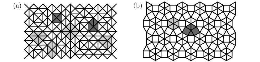
Figure 4.1: Residually convex tessellations of the plane. Residues of good ridges are shaded light. Residues of bad ridges are shaded dark. (a) A random tessellation by right isosceles triangles. Vertices of valency less than $6$ are bad ridges. (b) Vertices of squares are bad ridges.

One may observe that triangles contribute to such phenomena; this is the subject of the next subsection. Bounded convex domains may also admit such tessellations. For example, consider the tessellations of the Klein (projective) model of the hyperbolic plane corresponding to the triangle reflection groups $G(a,b,c)$ where $a=2$. In such tessellations, all $4$-valent vertices are bad ridges.

Later, we shall need the following fact that residual convexity is inherited by links.

Lemma 4.10.

Let $X$ be an $n$-complex and $e$ an $m$-cell of $X$ with $m<n$. If $X$ is residually convex then the link $\textup{Lk}(e;X)$ is residually convex.

Proof.

If $X$ is residually convex then $X$ is without boundary and the link $\textup{Lk}(e;X)$ is isometric to the sphere $\mathbb{S}^{n-m-1}$ (hence without boundary). Note first that every cell of the link $\textup{Lk}(e;X)$ is of the form $f_{(e;X)}$ for some cell $f$ of $X$. See (3.2.1). To check condition (3) in Lemma 4.1, let $\sigma_{(e;X)}$ be a facet of $\textup{Lk}(e;X)$ where $\sigma$ is a facet of $X$ containing $e$. Because an $n$-cell $P$ of $X$ contains $\sigma$ if and only if the corresponding $(n-m-1)$-cell $P_{(e;X)}$ of $\textup{Lk}(e;X)$ contains $\sigma_{(e;X)}$, we see that the residue of $\sigma_{(e;X)}$ in $\textup{Lk}(e;X)$ is equal to the link of $e$ in $res(\sigma;X)$, that is,

$$res(\sigma_{(e;X)};\textup{Lk}(e;X))=\textup{Lk}(e;res(\sigma;X)).$$

Because $X$ is residually convex, however, the residue $res(\sigma;X)$ is a convex $n$-polyball and hence the link $\textup{Lk}(e;res(\sigma;X))$ is also a convex $(n-m-1)$-polyball. The proof is complete. ∎

4.2 Complexes without triangular polytopes

We shall provide a simple combinatorial condition under which a given residually convex $n$-complex $X$ becomes strongly residually convex. In the following definition we regard a single polytope as a complex and its boundary as a subcomplex.

Definition 4.11 (Triangular polytopes).

A polytope $P$ is said to be triangular if it has a ridge $e$ and a face $f$ such that $res(e;\partial P)\cap f$ is disconnected. Such a pair $(e,f)$ is called a triangularity pair for $P$.

Of course, triangles are the only triangular $2$-polytopes. More discussion on (non-)triangular polytopes will be given after the proof of the following theorem.

Theorem 4.12.

Let $X$ be a residually convex $n$-complex. If none of the $n$-cells of $X$ is triangular, then $X$ is strongly residually convex.

Proof.

Let $e$ be a ridge of $X$ and let $F$ be a convex subcomplex in the boundary of $res(e)$ that does not intersect $e$. We shall show below that $F$ intersects either a single $n$-cell in $res(e)$ or two adjacent $n$-cells in $res(e)$ that share a common facet. It then follows that $st(F)\cap res(e)$ is a single $n$-cell or the residue of a facet. Because $X$ is residually convex, Lemma 4.1 (3) implies that $st(F)\cap res(e)$ is a convex $n$-polyball in either case, and we conclude that $e$ is a good ridge. Since $e$ is arbitrary, it then follows that $X$ is strongly residually convex.

As we observed in (3.4.5), we may set

$$res(e)=P_{1}\cup P_{2}\cup\cdots\cup P_{d_{e}}$$

so that $P_{i}$ and $P_{i+1}$ are adjacent and share a common facet $\sigma_{i}=P_{i}\cap P_{i+1}$, where the indices are taken modulo $d_{e}$. Moreover, we have $\sigma_{i}\cap\sigma_{j}=e$ for $i\neq j$. Because $F$ is a convex subcomplex in the boundary of $res(e)$ and $F$ does not intersect $e$, after cyclically permutating the indices of $P_{i}$, we may further assume that $F$ decomposes into

$$F=f_{1}\cup f_{2}\cup\cdots\cup f_{d}$$

for some $d<d_{e}$, where we define $f_{i}=F\cap P_{i}\neq\emptyset$. See Figure 4.2 (a).

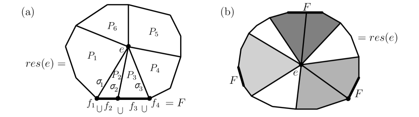
Figure 4.2: (a) Proof of Theorem 4.12. In this picture the convex subcomplex $F$ in the boundary of $res(e)$ intersects $P_{1},\ldots,P_{4}$, hence $d=4$. As the proof shows, the polytope $P_{2}$ (as well as $P_{3}$) is triangular. (b) Illustration of Theorem 4.12. If there is no triangular polytope in $res(e)$, then convex subcomplexes $F$ in its boundary intersect at most two $n$-cells. It follows from residual convexity that the ridge $e$ is good.

We then observe the following:

• For each $1\leq i\leq d$ the cell $f_{i}$ is convex because $F$ and $P_{i}$ are convex. If the dimension of $f_{i}$ is $m$, then $f_{i}$ is a single $m$-cell in $P_{i}$ because $P_{i}$ is a (convex) polytope;

• For each $1\leq i\leq d-1$ the intersection $f_{i}\cap f_{i+1}$ is a non-empty subset of $\sigma_{i}$, because $F$ is connected and

  $$f_{i}\cap f_{i+1}=(F\cap P_{i})\cap(F\cap P_{i+1})=F\cap(P_{i}\cap P_{i+1})=F\cap\sigma_{i}\subset\sigma_{i}.$$

Suppose now that $F$ intersects more than two $n$-cells in $res(e)$, that is, $d\geq 3$. We then have $f_{1}\cap f_{2}\subset\sigma_{1}$ and $f_{2}\cap f_{3}\subset\sigma_{2}$. Because $\sigma_{1}\cap\sigma_{2}=e$ and $F$ does not intersect $e$, we see that $f_{1}\cap f_{2}$ and $f_{2}\cap f_{3}$ are disjoint. However, since $\sigma_{1}\cap f_{2}\subset P_{1}\cap F=f_{1}$ and $\sigma_{2}\cap f_{2}\subset P_{3}\cap F=f_{3}$, we have $\sigma_{1}\cap f_{2}=f_{1}\cap f_{2}$ and $\sigma_{2}\cap f_{2}=f_{2}\cap f_{3}$. It follows that

$$res(e,\partial P_{2})\cap f_{2} =(\sigma_{1}\cup\sigma_{2})\cap f_{2}$$

$$=(\sigma_{1}\cap f_{2})\cup(\sigma_{2}\cap f_{2})$$

$$=(f_{1}\cap f_{2})\cup(f_{2}\cap f_{3})$$

is disconnected; a contradiction because $e\subset P_{2}$ is a ridge, $f_{2}\subset P_{2}$ is a single $m$-cell, and $P_{2}$ is not triangular. Therefore, we must have $d\leq 2$ and $F$ intersects either $P_{1}$ or $P_{1}\cup P_{2}=res(\sigma_{1})$. This completes the proof of the assertion at the beginning. ∎

Combining the above with Theorem 4.8 we have the following immediate corollary:

Corollary 4.13.

Let $X$ be a residually convex $n$-complex. If none of the $n$-cells of $X$ is triangular, then $X$ is isometric to a convex proper domain in $\mathbb{S}^{n}$. In particular, $X$ is contractible.

Remark 4.14.

In fact, the proof of Theorem 4.8 shows that the conclusion of Corollary 4.13 is still valid when $X$ is allowed to have a single triangular polytope. Namely, we can take the single triangular polytope to be the initial polytope $P_{0}$ in the proof of Theorem 4.8.

The following corollary provides us with a necessary condition for residual convexity:

Corollary 4.15.

Let $X$ be a residually convex $n$-complex and $e$ an $m$-cell of $X$ with $m\leq n-3$. Then the link $\textup{Lk}(e;X)$ contains a triangular $(n-m-1)$-polytope.

Proof.

By Lemma 4.10 the link $\textup{Lk}(e;X)$ is a residually convex $(n-m-1)$-complex which is isometric to the sphere $\mathbb{S}^{n-m-1}$. If $\textup{Lk}(e;X)$ contained no triangular polytope, then it would be contractible by the previous corollary. Because spheres are not contractible, the link $\textup{Lk}(e;X)$ must contain a triangular polytope. ∎

Thus, for example, one cannot obtain a residually convex $3$-complex by gluing together copies of octahedra only.

Remark 4.16.

(1) The previous corollary suggests that it would be good if one could catalogue all residually convex tessellations of the sphere $\mathbb{S}^{n}$.

(2) As we observed in the introduction, a residually convex complex may fail to be strongly residually convex if it contains triangular polytopes. See Figure 1.3 (b). See also Remark 4.9 (2) and Figure 4.1, where we provided some examples of residually convex tessellations of the plane which are not strongly residually convex.

(3) It would be of independent interest to know if every (convex or non-convex) domain can admit a residually convex tessellation. Note that Figure 1.1 is just a feasible picture of a non-convex domain admitting a residually convex tessellation. In addition to Figure 1.3 (b), we provide in Figure 4.3 more examples of non-convex domains admitting a residually convex tessellation.

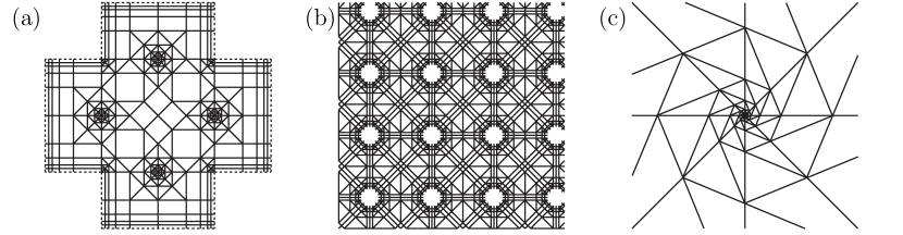
Figure 4.3: Non-convex domains admitting a residually convex tessellation. (a) A (cross-shaped) bounded domain with four punctures. (b) The plane with a lattice of octagons removed. (c) A variant of Benoist’s example in Figure 1.3 (b).

Example 4.17 (Triangular polytopes).

(1) Triangles are the only triangular $2$-polytopes. Pyramids are triangular; they are cone-like (see Definition 5.6 and Lemma 5.7). Prisms over triangular polytopes are also triangular because if $(e,f)$ is a triangularity pair for $P$ then so too is $(e\times I,f\times I)$ for $P\times I$.

(2) Let $P$ be an $n$-polytope and $v$ a vertex of $P$. If the link $\textup{Lk}(v;P)$ is a triangular $(n-1)$-polytope then the polytope $P^{\prime}$ obtained by truncating the vertex $v$ of $P$ is also triangular. Indeed, if $e$ is a ridge and $f$ is a face of $P$ such that $(e_{(v;P)},f_{(v;P)})$ is a triangularity pair for the link $\textup{Lk}(v;P)$, then the pair of truncated faces $(e^{\prime},f^{\prime})$ is a triangularity pair for $P^{\prime}$. Thus, for example, if $v$ is a simple vertex of $3$-polytope $P$, that is, $v$ is contained in exactly $3$ facets of $P$, then the polytope $P^{\prime}$ obtained by truncating $v$ of $P$ is triangular. (In this case, $(P^{\prime})^{*}$ is also triangular.) See Figure 4.4 (a) and (b). Of course, not all triangular polytopes are obtainable by this procedure. See Figure 4.4 (c).

Figure 4.4: (a) Illustration of the claim in Example 4.17 (2). The truncated cube $P^{\prime}$ is triangular. (b) If a $3$-polytope $P$ has a triangular facet with a simple ($3$-valent) vertex, then its dual $P^{*}$ has the same property. In this case, both $P$ and $P^{*}$ are triangular. (c) A simple triangular $3$-polytope without triangular facets.

Example 4.18 (Non-triangular polytopes).

(1) Examples of non-triangular polytopes include $k$-gons ($k>3$), Platonic solids other than tetrahedra, and prisms over non-triangular polyhedra.

(2) One can transform any triangular polytope $P$ into a non-triangular polytope as follows. Let $(e,f)$ be a triangularity pair for $P$. The plan is to keep $e$ intact and break $f$ into pieces so that no face of the new polytope $\hat{P}$ can give rise to a triangularity pair with $e$. More precisely, let $f$ be a minimal (with respect to inclusion) face of $P$ such that $(e,f)$ is a triangularity pair for $P$. Place a vertex $v\in\mathbb{S}^{n}$ in the exterior of $P$ arbitrarily close to the barycenter of $f$. The new polytope $\hat{P}$ is obtained by ”raising a pyramid” over the residue $res(f;\partial P)$ with apex $v$. That is, we raise pyramids with common apex $v$ over every face in the residue $res(f;\partial P)$. See Figure 4.5.

Figure 4.5: (a) A truncated cube $P$ with triangularity pair $(e,f)$. (b) Raising a pyramid over $res(f;\partial P)$, one obtains a polytope $P^{\prime}$ which has a triangularity pair $(e_{1},f_{1})$. (c) Finally, raising a pyramid over $res(f_{1};\partial P^{\prime})$, one obtains a polytope $P^{\prime\prime}$ which is non-triangular.

This procedure adds only a single vertex $v$ and does not change the ridge $e$. If we keep doing this procedure for each minimal face $f$ with respect to $e$ and then the same procedure for all ridges $e$ of $P$, then we eventually get a non-triangular polytope.

(3) Similar reasoning shows that if we put new vertices $v_{f}$ over all $i$-faces $f$ of $P$ ($i\neq 0,n$) and raise pyramids simultaneously over $f$ with apex $v_{f}$, then we get a non-triangular polytope $\hat{P}$ whose boundary $\partial\hat{P}$ is combinatorially equal to the one which is obtained by performing barycentric subdivision on the boundary $\partial P$ of the old polytope $P$.

(4) Finally, in terms of duality the (non-)triangularity condition translates as follows:

$P$ is non-triangular if and only if its dual $P^{*}$ satisfies the property that, for each edge $e^{*}$ in $P^{*}$, the set $st(e^{*};\partial P^{*})\setminus res(e^{*};\partial P^{*})$ is disconnected.

To see this, first notice that $e$ is a ridge of $P$ if and only if $e^{*}$ is an edge of $P^{*}$. Indeed, $\sigma_{1}$ and $\sigma_{2}$ are facets of $P$ such that $\sigma_{1}\cap\sigma_{2}=e$ if and only if $\sigma_{1}^{*}$ and $\sigma_{2}^{*}$ are vertices of $P^{*}$ spanning an edge $e^{*}$. In this case, we have

$$res(e^{*};\partial P^{*}) \subset st(\sigma_{1}^{*};\partial P^{*})\cap st(\sigma_{2}^{*};\partial P^{*});$$

$$st(e^{*};\partial P^{*}) =st(\sigma_{1}^{*};\partial P^{*})\cup st(\sigma_{2}^{*};\partial P^{*}),$$

which follows immediately from the definition. Because $P^{*}$ is a (convex) polytope, however, the vertex stars $st(\sigma_{1}^{*};\partial P^{*})$ and $st(\sigma_{2}^{*};\partial P^{*})$ are topological balls. Therefore, the set $st(e^{*};\partial P^{*})\setminus res(e^{*};\partial P^{*})$ is disconnected if and only if we have

$$res(e^{*};\partial P^{*})=st(\sigma_{1}^{*};\partial P^{*})\cap st(\sigma_{2}^{*};\partial P^{*}).$$

We now begin to prove the assertion made at the beginning. From the previous discussion, we know that the set $st(e^{*};\partial P^{*})\setminus res(e^{*};\partial P^{*})$ is connected for some edge $e^{*}$ of $P^{*}$ if and only if there are faces $f_{1}^{*}$ and $f_{2}^{*}$ of $P^{*}$ such that

• for each $i=1,2$, $f_{i}^{*}\subset st(\sigma_{i}^{*};\partial P^{*})$, that is, $\sigma_{i}^{*}$ is a vertex of $f_{i}^{*}$;

• $f^{*}:=f_{1}^{*}\cap f_{2}^{*}$ is not contained in $res(e^{*};\partial P^{*})$, that is, there is no facet of $P^{*}$ containing both $e^{*}$ and $f^{*}$.

In terms of duality, this is equivalent to the condition that there is a face $f$ of $P$ such that

• for each $i=1,2$, $f_{i}$ is a face of the facet $\sigma_{i}$ of $P$;

• $f_{1}$ and $f_{2}$ are faces of $f$, and $f$ is disjoint from $e$.

In other words, there is a face $f$ of $P$ such that $f\cap\sigma_{1}=f_{1}$ is disjoint from $f\cap\sigma_{2}=f_{2}$, hence $(e,f)$ is a triangularity pair for $P$ and $P$ is triangular.

(5) For example, let $P$ be a simple $n$-polytope, that is, every vertex of $P$ is contained in exactly $n$ facets of $P$. Then the facets of the dual $P^{*}$ are all $(n-1)$-simplices. Then the set $st(e^{*};\partial P^{*})\setminus res(e^{*};\partial P^{*})$ is connected for some edge $e^{*}$ if and only if either $P^{*}$ has a simple $m$-simplex ($m<n-2$) or $\partial P^{*}$ has an edge-path of length $3$ that does not bound a $2$-simplex. In conclusion, a simple polytope $P$ is non-triangular if and only if $P$ has no $m$-simplex ($m>1$) and $\partial P^{*}$ has no nontrivial edge-path of length $3$. Figure 4.4 (c) shows a simple $3$-polytope with no triangular facet but with a nontrivial edge-path of length $3$ in the boundary of its dual.

5 Proper convexity

In this section we shall study only those residually convex $n$-complexes $X$ which have no triangular $n$-cells. From Corollary 4.13 we know that $X$ is isometric to a convex proper domain in $\mathbb{S}^{n}$. Thus we may identify $X$ with its image $dev(X)\subset\mathbb{S}^{n}$ and regard $X$ as a subset of $\mathbb{S}^{n}$. The goal of this section is to prove the following theorem.

Theorem 5.1.

Let $X\subset\mathbb{S}^{n}$ be a residually convex $n$-complex such that none of the $n$-cells of $X$ are triangular. If $X$ has an $n$-cell $Q$ whose dual $Q^{*}$ is thick, then $X$ is a properly convex domain in $\mathbb{S}^{n}$.

Before we proceed to prove the above theorem, we introduce thick polytopes and discuss some of their examples.

Definition 5.2 (Thick polytopes).

Let $P\subset\mathbb{S}^{n}$ be an $n$-polytope. We call $P$ thin provided that there is a hyperplane $H\subset\mathbb{S}^{n}$ (called a cutting plane for $P$) which contains no vertices of $P$ such that the following condition is satisfied by all vertices $v$ of $P$:

if the vertex $v$ is in one halfspace determined by $H$ then there is another vertex $v^{\prime}$ in the other halfspace that is connected to $v$ by an edge.

An $n$-polytope is said to be thick if it is not thin.

Remark 5.3.

Of course, by dualizing Definition 5.2, we could state Theorem 5.1 without mentioning the dual $Q^{*}$ of $Q$. We adopted the current approach, however, because the dualized definition is less intuitive:

the dual $P^{*}$ of an $n$-polytope $P$ is thin if and only if there is a point $x\in\mathbb{S}^{n}$ such that, for each facet $\sigma$ of $P$, the hyperplane $\langle\sigma\rangle$ spanned by $\sigma$ does not contain $x$ and if $x$ is in the halfspace $\langle\sigma\rangle^{\pm}$ then $x$ is in $\langle\sigma^{\prime}\rangle^{\mp}$ for some facet $\sigma^{\prime}$ adjacent to $\sigma$.

Example 5.4 (Thin polytopes).

Figure 5.1 shows some examples of thin polytopes. It is clear that triangles and quadrilaterals are the only thin $2$-polytopes. Pyramids, bipyramids and prisms are thin (see Lemma 5.14 below). The regular icosahedron is also thin.

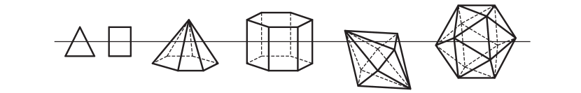
Figure 5.1: Thin polytopes. The horizontal line represents the cutting plane.

Remark 5.5 (Thick polytopes).

Definition 5.2 suggests that polytopes with more combinatorial complexity would have better chance to be thick and, in some sense, thick polytopes are much more common than thin ones. But it is rather hard to find simple combinatorial conditions which imply thickness of polytopes.

In [13] we classify thin simple $3$-polytopes and show that they must contain a triangular or quadrilateral facet. Furthermore, both thin simple $3$-polytopes and their dual polytopes turn out to have Hamiltonian cycles. These facts imply that, for example, dodecahedron, truncated icosahedron (soccer ball) and Tutte’s non-Hamiltonian simple polytopes are thick.

To prove the above theorem we need some preparation. In the following Sections 5.1-5.3 we study more about residually convex $n$-complexes without triangular $n$-cells and develop a few related notions. The proof of Theorem 5.1 is then provided in the end of Section 5.3.

5.1 Cone-like polytopes

The following definition and lemma are essential to the subsequent constructions.

Definition 5.6 (Cone-like polytopes).

A polytope $P$ is said to be cone-like if it has a facet $\sigma$ such that $st(\sigma;\partial P)=\partial P$.

Recall that the boundary $\partial P$ of a polytope $P$ is the union of facets of $P$. Thus if $P$ is cone-like with respect to some facet $\sigma$ then all facets of $P$ intersect $\sigma$. See Figure 5.2.

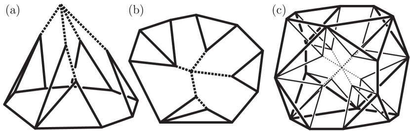
Figure 5.2: Cone-like polytopes with $\Sigma$ dashed. (a) A cone-like $3$-polytope. (b) A Schlegel diagram of the polytope in (a). (c) A Schlegel diagram of a $4$-polytope whose $\Sigma$ is $1$-dimensional. This $4$-polytope has $15$ facets.

Lemma 5.7.

Cone-like polytopes are triangular.

Proof.

Suppose that $P$ is a cone-like $n$-polytope and $\sigma$ is a side of $P$ such that $st(\sigma;\partial P)=\partial P$. The boundary $\partial P$ of $P$ is topologically an $(n-1)$-dimensional sphere with cell structure induced from the faces of $P$. Let $\Sigma\subset\partial P$ be the union of all faces of $P$ that are disjoint from $\sigma$. Because all facets of $P$ intersect $\sigma$, the dimension of $\Sigma$ is at most $n-2$.

Case I. If $\Sigma$ has dimension $n-2$, choose any ridge $e$ of $P$ in $\Sigma$. Denote by $\sigma_{1}$ and $\sigma_{2}$ the two adjacent facets of $P$ along $e$. Because $\sigma_{1}\cap\sigma_{2}=e$ is disjoint from $\sigma$, we see that

$$res(e;\partial P)\cap\sigma =(\sigma_{1}\cup\sigma_{2})\cap\sigma$$

$$=(\sigma_{1}\cap\sigma)\cup(\sigma_{2}\cap\sigma)$$

is disconnected. Therefore, $P$ is triangular.

Case II. If $\Sigma$ has dimension $k$ with $k<n-2$, all faces of $P$ of dimension $>k$ intersect $\sigma$. Let $\sigma^{\prime}$ be a facet of $P$ other than $\sigma$. Let $e=\sigma\cap\sigma^{\prime}$ be a face of $P$. Because all ridges of $P$ intersect $\sigma$, all facets of $\sigma^{\prime}$ intersect $\sigma$ and hence $e$. Thus we have $st(e;\partial\sigma^{\prime})=\partial\sigma^{\prime}$. It follows that $e$ is a facet of $\sigma^{\prime}$ (hence, a ridge of $P$), $\sigma^{\prime}$ is cone-like with respect to $e$ and that $res(e;\partial P)=\sigma\cup\sigma^{\prime}$. Now, because the dimension of $\Sigma$ is $k$, we can choose a $(k+1)$-dimensional face $f$ of $P$ so that $\sigma^{\prime}\cap f\neq\emptyset$ and $\sigma^{\prime}\cap f\subset\Sigma$. Then, because all faces of $P$ of dimension $>k$ intersect $\sigma$, the intersection $\sigma\cap f$ is non-empty and disjoint from $\sigma^{\prime}\cap f\subset\Sigma$. We thus have that

$$res(e;\partial P)\cap f =(\sigma\cup\sigma^{\prime})\cap f$$

$$=(\sigma\cap f)\cup(\sigma^{\prime}\cap f)$$

is disconnected and hence that $P$ is triangular. ∎

Remark 5.8.

Not all triangular polytopes are cone-like. Such examples can be seen in Figure 4.4 (a) and (c).

5.2 Directed galleries and supporting hyperplanes

From now on we assume that $X\subset\mathbb{S}^{n}$ is a residually convex $n$-complex such that none of the $n$-cells of $X$ is triangular. It follows from Lemma 5.7 that no $n$-cells of $X$ are cone-like; this fact enables us to consider the following objects in $X$.

We fix a specified $n$-cell $Q$ in $X$. Let $\sigma$ be a facet of $Q$. Then there is an $n$-cell $P_{1}$ of $X$ adjacent to $Q$ along $\sigma$. Because $P_{1}$ is not cone-like, we can choose a facet $s_{1}$ of $P_{1}$ which is disjoint from $\sigma$. Then there is an $n$-cell $P_{2}$ adjacent to $P_{1}$ along $s_{1}$. Because $P_{2}$ is not cone-like, $P_{2}$ has a facet $s_{2}$ which is disjoint from $s_{1}$. Continuing in this manner we obtain two infinite sequences $\{P_{j}\}$ of $n$-cells and $\{s_{j}\}$ of facets such that $P_{j}\cap P_{j+1}=s_{j}$ for all $j\geq 0$, where we set $P_{0}=Q$ and $s_{0}=\sigma$. See Figure 5.3. This motivates the following definition:

Figure 5.3: A directed gallery from $Q$ in the direction of $\sigma$.

Definition 5.9 (Directed galleries).

A directed gallery $Gal_{(Q,\sigma)}(P_{j},s_{j})$ from $Q$ in the direction of $\sigma$ is the union $\bigcup_{j=0}^{\infty}P_{j}$ of an infinite family of $n$-cells of $X$ such that for each $j\geq 0$

• $P_{j}\cap P_{j+1}=s_{j}$ is a facet of $X$, where $P_{0}=Q$ and $s_{0}=\sigma$;

• $s_{j}\cap s_{j+1}=\emptyset$.

Thus the previous discussion says that to each facet $\sigma$ of $Q$ we can associate a directed gallery $Gal_{(Q,\sigma)}(P_{j},s_{j})$ from $Q$ in the direction of $\sigma$. Of course, because of the choices of $s_{j}$ we made, the directed galleries are not uniquely determined by $Q$ and $\sigma$. The lemma below, however, shows that they satisfy a common property in relation to the iterated stars $st^{j}(Q)$ of $Q$ in $X$.

First notice the following. Because $X$ is strongly residually convex by Theorem 4.12, the proof of Theorem 4.8 applied to $X$ and $Q$ shows that the iterated stars $st^{j}(Q)$ are convex $n$-polyballs. Recall that $X$ is assumed to be a subset of $\mathbb{S}^{n}$. Thus the stars $st^{j}(Q)$ form a nested sequence of closed $n$-dimensional convex proper subsets of $\mathbb{S}^{n}$.

Lemma 5.10.

Let $Gal_{(Q,\sigma)}(P_{j},s_{j})$ be a directed gallery from $Q$ in the direction of $\sigma$. Then the following assertions are true:

1. Each facet $s_{j}$ ($j\geq 0)$ is in the boundary of the star $st^{j}(Q)$ of $Q$.

2. The gallery $Gal_{(Q,\sigma)}(P_{j},s_{j})$ is a convex subset of $\mathbb{S}^{n}$.

Proof.

(1) The proof is by induction on $j\geq 0$. When $j=0$, it is clear that $s_{0}=\sigma$ is in the boundary of $st^{0}(Q)=Q$. Now assume that the conclusion is true up to the $(j-1)$-th step. We need to show that $s_{j}$ is in the boundary of $st^{j}(Q)$.

Because $P_{j}$ intersects $st^{j-1}(Q)$ at $s_{j-1}$, we have that

$$s_{j}\subset P_{j}\subset st[st^{j-1}(Q)]=st^{j}(Q).$$

To show that $s_{j}$ is in the boundary of $st^{j}(Q)$, consider the residue $res(s_{j})=P_{j}\cup P_{j+1}$. It is a convex subset of $\mathbb{S}^{n}$ by residual convexity of $X$. Moreover, it contains $s_{j-1}$ in its boundary, since $s_{j-1}$ is a facet of $P_{j}$:

$$s_{j-1}\subset\partial(P_{j}\cup P_{j+1})=\partial res(s_{j}).$$

However, $s_{j-1}$ is disjoint from $s_{j}$ and hence from $P_{j+1}$. Because $P_{j}$ is a convex polytope, it follows that $s_{j-1}$ is a maximal convex subset in the boundary of $res(s_{j})$. Now, by the induction hypothesis, $s_{j-1}$ is also contained in the boundary of the convex subset $st^{j-1}(Q)$. From the convexity of $res(s_{j})$ and $st^{j-1}(Q)$, and from the maximality of $s_{j-1}$, it follows that

$$res(s_{j})\cap st^{j-1}(Q)=s_{j-1}.$$

Thus $P_{j+1}$ is disjoint from $st^{j-1}(Q)$ and cannot intersect the interior of the star $st^{j}(Q)$. In particular, $s_{j}\subset P_{j+1}$ does not intersect the interior of $st^{j}(Q)$ and hence must be in the boundary of $st^{j}(Q)$. The induction is complete.

(2) Let $G_{k}=\bigcup_{j=0}^{k}P_{j}$. The previous proof of (1) shows that $G_{k}$ is contained in $st^{k}(Q)$ and intersects $P_{k+1}$ exactly along $\sigma_{k}$. These facts inductively imply that $G_{k}$ is an $n$-polyball for all $k\geq 0$. Now, fix $k$ and let $e$ be a ridge in the boundary of $G_{k}$. From the construction of galleries, it is clear that $e$ intersects either a single $n$-cell of $G_{k}$ or two adjacent $n$-cells of $G_{k}$. In either case, the residual convexity of $X$ implies that the link $\textup{Lk}(e;G_{k})$ is convex. Since $e$ is arbitrary, it follows from Lemma 3.4 that the polyball $G_{k}$ is convex. Since $k$ is arbitrary, $G_{k}$ is convex for all $k\geq 0$. Because the nested sequence $\{G_{k}\}$ exhausts the gallery $Gal_{(Q,\sigma)}(P_{j},s_{j})$, the conclusion follows. ∎

Recall that we fixed a specified $n$-cell $Q$ in $X$. Let $\sigma$ be a facet of $Q$. Let $Gal_{(Q,\sigma)}(P_{j},s_{j})$ be a directed gallery from $Q$ in the direction of $\sigma$. The above lemma says that each facet $s_{j}$ in this gallery is in the boundary of the star $st^{j}(Q)$. Denote by $\langle s_{j}\rangle$ the hyperplane spanned by $s_{j}$. Because $st^{j}(Q)$ is convex, $\langle s_{j}\rangle$ must be a supporting hyperplane of $st^{j}(Q)$. Now consider the sequence $\{\langle s_{j}\rangle\}$ of hyperplanes of $\mathbb{S}^{n}$. Because $\mathbb{S}^{n}$ is compact this sequence converges to a hyperplane which we denote by

$$H_{X}(\sigma).$$ (5.2.1)

Because the convex sets $st^{j}(Q)$ exhaust $X$ and their supporting hyperplanes $\langle s_{j}\rangle$ converge to $H_{X}(\sigma)$, it immediately follows that $H_{X}(\sigma)$ is a supporting hyperplane of the convex subset $X\subset\mathbb{S}^{n}$. See Figure 5.4 (a).

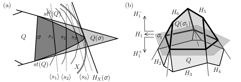
Figure 5.4: (a) To each facet $\sigma$ of $Q$ we can associate a directed gallery $Gal_{(Q,\sigma)}(P_{j},s_{j})$ in the direction of $\sigma$, which again determines a supporting hyperplane $H_{X}(\sigma)$ of $X$. (b) To each facet $\sigma_{1}$ of $Q$ we can assign a cone-like polytope $Q(\sigma_{1})$.

In this manner, to each facet $\sigma$ of $Q$, we can assign a supporting hyperplane $H_{X}(\sigma)$ of $X$. Notice that the hyperplane $H_{X}(\sigma)$ is not uniquely determined by the facet $\sigma$ because the associated gallery is not uniquely determined by $\sigma$ either. Therefore, we are rather interested in all possible locations of $H_{X}(\sigma)$ in $\mathbb{S}^{n}$. As will be explained below, the restriction on their location is given by the specified $n$-cell $Q$ and its facets.

We may assume that the $n$-cell $Q\subset X$ is expressed as

$$Q=\bigcap_{i=1}^{m}H_{i}^{+},$$

where $m\geq n+1$ and the $\{H_{i}^{+}\}$ is an irredundant family of halfspaces bounded by hyperplanes $H_{i}$. Then the facets $\sigma_{i}$ of $Q$ are of the form $\sigma_{i}=Q\cap H_{i}$ for $1\leq i\leq m$.

Consider the facet $\sigma_{1}$ of $Q$. Let $\sigma_{2},\sigma_{3},\ldots,\sigma_{k}$ ($k<m$) be the facets of $Q$ that are adjacent to $\sigma_{1}$ along ridges. Consider the $n$-polytope $Q(\sigma_{1})$ defined as the intersection of the $k$ halfspaces $H_{1}^{-},H_{2}^{+},\ldots,H_{k}^{+}$:

$$Q(\sigma_{1})=H_{1}^{-}\cap H_{2}^{+}\cap\cdots\cap H_{k}^{+}.$$ (5.2.2)

See Figure 5.4 (b). (The polytope $Q(\sigma_{1})$ is cone-like and its vertices in $\sigma_{1}$ are simple.) Consider also a directed gallery $Gal_{(Q,\sigma_{1})}(P_{j},s_{j})$ from $Q$ in the direction of $\sigma_{1}$. By Lemma 5.10 (2), it is a convex subset of $\mathbb{S}^{n}$. However, the $(k-1)$ hyperplanes $H_{2},\ldots,H_{k}$ support $Q$ and hence $Gal_{(Q,\sigma_{1})}(P_{j},s_{j})$. It follows that the set $Gal_{(Q,\sigma_{1})}(P_{j},s_{j})\setminus Q$ is contained in the polytope $Q(\sigma_{1})$:

$$\bigcup_{j=1}^{\infty}P_{j}=Gal_{(Q,\sigma_{1})}(P_{j},s_{j})\setminus Q\subset Q(\sigma_{1}).$$

Recall that each hyperplane $\langle s_{j}\rangle$ supports the star $st^{j}(Q)$ of $Q$. Thus no $\langle s_{j}\rangle$ ($j\geq 1$) can intersect a neighborhood of $Q$ (namely, the interior of $st(Q)$) but always intersects the interior of $Q(\sigma_{1})$. Being the the limit of the hyperplanes $\langle s_{j}\rangle$, the hyperplane $H_{X}(\sigma_{1})$ cannot intersect $Q$ but must intersect $Q(\sigma_{1})$. See Figure 5.4 (a).

If we define $Q(\sigma_{i})$ analogously for each facet $\sigma_{i}$ of $Q$, the analogous statements hold for the hyperplanes $H_{X}(\sigma_{i})$:

Lemma 5.11.

Given an $n$-cell $Q$ in $X$, the hyperplanes $H_{X}(\sigma_{i})$ and the $n$-polytopes $Q(\sigma_{i})$ associated to facets $\sigma_{i}$ of $Q$ satisfy the following relations: for all $i$,

$$H_{X}(\sigma_{i})\cap Q=\emptyset\quad\text{and}\quad H_{X}(\sigma_{i})\cap Q(\sigma_{i})\neq\emptyset.$$

These restrictions on the location of $H_{X}(\sigma_{i})$ are more conveniently described in terms of duality, since the duals of the halfspaces determined by $H_{X}(\sigma_{i})$ are just points. The next subsection is devoted to this description.

5.3 Pavilions and $n+1$ hyperplanes in general position

We continue to assume that $X\subset\mathbb{S}^{n}$ is a residually convex $n$-complex such that none of its $n$-cells is triangular and that $Q$ is a fixed $n$-cell in $X$. In our previous discussion we expressed the $n$-cell $Q$ as

$$Q=\bigcap_{i=1}^{m}H_{i}^{+}.$$

Now, denote by $v_{i}=(H_{i}^{+})^{*}$ the dual of the halfspace $H_{i}^{+}$. Then each $v_{i}$ becomes a vertex of the dual polytope $Q^{*}$ of $Q$ (see Section 2.5):

$$Q^{*}=\left[\bigcap_{i=1}^{m}H_{i}^{+}\right]^{*}=\textup{conv}\left[\bigcup_{i=1}^{m}(H_{i}^{+})^{*}\right]=\textup{conv}\{v_{1},v_{1},\ldots,v_{m}\}.$$

Recall also the definition (5.2.2) of the $n$-polytope $Q(\sigma_{1})$ associated to the facet $\sigma_{1}$ of $Q$:

$$Q(\sigma_{1})=H_{1}^{-}\cap H_{2}^{+}\cap\cdots\cap H_{k}^{+}.$$

Its dual $Q(\sigma_{1})^{*}$ is the convex hull of the vertices $v_{2},\ldots,v_{k}$ and $-v_{1}$, where $-v_{1}=(H_{1}^{-})^{*}$ is the antipodal point of $v_{1}$ (see Section 2.5):

$$Q(\sigma_{1})^{*} =\left(H_{1}^{-}\cap H_{2}^{+}\cap\cdots\cap H_{k}^{+}\right)^{*}$$

$$=\textup{conv}\left\{(H_{1}^{-})^{*},(H_{2}^{+})^{*},\ldots,(H_{k}^{+})^{*}\right\}$$

$$=\textup{conv}\{-v_{1},v_{2},\ldots,v_{k}\}.$$

Note that the vertices $v_{2},\ldots,v_{k}$ of $Q(\sigma_{1})^{*}$ (and $Q^{*}$) are connected to $v_{1}$ by the edges of $Q^{*}$ which are dual to the ridges $\sigma_{1}\cap\sigma_{i}$ ($2\leq i\leq k$) of $Q$.

Recall the definition (5.2.1) of the supporting hyperplane $H_{X}(\sigma_{1})$ of $X$ associated to the facet $\sigma_{1}$ of $Q$. Now let $H_{X}(\sigma_{1})^{+}$ be the halfspace which is bounded by $H_{X}(\sigma_{1})$ and which contains the $n$-complex $X$. Denote by $x(\sigma_{1})=[H_{X}(\sigma_{1})^{+}]^{*}$ the dual point of $H_{X}(\sigma_{1})^{+}$. In Lemma 5.11 we summarized the restrictions on the position of $H_{X}(\sigma_{1})$. Dualizing these we obtain the following conditions on the location of $x(\sigma_{1})$:

Because $H_{X}(\sigma_{1})^{+}$ contains $Q$ but $H_{X}(\sigma_{1})$ does not intersect $Q$, the point $x(\sigma_{1})$ must be in the interior of $Q^{*}$. On the other hand, because $H_{X}(\sigma_{1})$ intersects $Q(\sigma_{1})$, the point $x(\sigma_{1})$ cannot be an interior point of $Q(\sigma_{1})^{*}$.

These restrictions on $x(\sigma_{1})$ motivate the following definition. Recall that $S^{\circ}$ denotes the interior of a set $S$.

Definition 5.12 (Pavilion).

Let $P$ be an $n$-polytope in $\mathbb{S}^{n}$. Let $v$ be a vertex of $P$ and let $V(v)$ be the set of all vertices of $P$ that are connected to $v$ by edges of $P$. Denote by $P(v)=\textup{conv}\left(\{-v\}\cup V(v)\right)$ the convex hull of $-v$ and $V(v)$. The pavilion $\textup{pv}(v;P)$ of $v$ in $P$ is by definition

$$\textup{pv}(v;P)=P^{\circ}\setminus P(v)^{\circ}.$$

The base $\underline{\textup{pv}}(v;P)$ of the pavilion $\textup{pv}(v;P)$ is defined as

$$\underline{\textup{pv}}(v;P)=P^{\circ}\cap\partial P(v).$$

Note that the base $\underline{\textup{pv}}(v;P)$ is an open subset of $\partial P(v)$. See Figure 5.5.

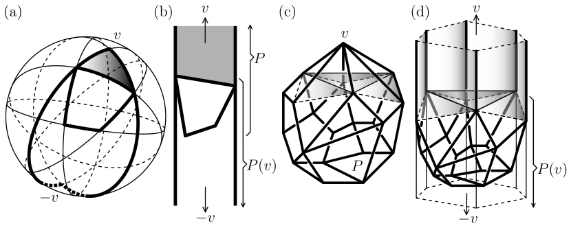
Figure 5.5: Pavilions. (a) $P$ is a pentagon with $\textup{pv}(v;P)$ shaded. (b) A view of (a) in an affine $2$-plane. (c) $P$ is a $3$-polytope. The base $\underline{\textup{pv}}(v;P)$ of a pavilion is shaded and consists of four triangles. (d) A view of (c) in an affine $3$-plane. The six facets containing $v$ determine a hexagonal cylinder. The pavilion $\textup{pv}(v;P)$ is shaded.

To summarize, the point $x(\sigma_{1})=[H_{X}(\sigma_{1})^{+}]^{*}$ we considered above must be in the pavilion $\textup{pv}(v_{1};Q^{*})$ of $v_{1}$ in $Q^{*}$. Similarly, by considering the analogous restrictions on $H_{X}(\sigma_{i})$ with respect to $Q$ and $Q(\sigma_{i})$ given by Lemma 5.11, we obtain the following.

Lemma 5.13.

Let $Q$ be an $n$-cell in $X$. For each facet $\sigma_{i}$ of $Q$ ($1\leq i\leq m$), let $H_{X}(\sigma_{i})$ be the supporting hyperplanes of $X$ associated to $\sigma_{i}$. Let $H_{X}(\sigma_{i})^{+}$ denote the halfspace which is bounded by $H_{X}(\sigma_{i})$ and which contains the $n$-complex $X$. Then, for all $i$, the dual points of $H_{X}(\sigma_{1})^{+}$

$$x(\sigma_{i})=[H_{X}(\sigma_{i})^{+}]^{*}$$

must satisfy

$$x(\sigma_{i})\in\textup{pv}(v_{i};Q^{*}).$$

Assuming another Lemma 5.14 below, we are now ready to prove Theorem 5.1.

Proof of Theorem 5.1.

Let $Q$ be the $n$-cell of $X$ whose dual $Q^{*}$ is thick. As before, we may assume that the $n$-cell $Q\subset X$ is expressed as

$$Q=\bigcap_{i=1}^{m}H_{i}^{+},$$

where $m\geq n+1$ and the $\{H_{i}^{+}\}$ is an irredundant family of halfspaces bounded by hyperplanes $H_{i}$. Then the facets $\sigma_{i}$ of $Q$ are of the form $\sigma_{i}=Q\cap H_{i}$ for $1\leq i\leq m$ and the vertices of the dual $Q^{*}$ are $v_{i}=(H_{i}^{+})^{*}$.

As in Section 5.2, for each facet $\sigma_{i}$ of $Q$, we choose a directed gallery from $Q$ in the direction of $\sigma_{i}$ to obtain a supporting hyperplane $H_{X}(\sigma_{i})$ of $X$. We let $x(\sigma_{i})=[H_{X}(\sigma_{i})^{+}]^{*}$ be the dual point of $H_{X}(\sigma_{i})^{+}$. Then Lemma 5.13 tells us that

$$x(\sigma_{i})\in\textup{pv}(v_{i};Q^{*})$$

for all $1\leq i\leq m$.

Suppose by way of contradiction that the $m$ points $x(\sigma_{i})$ are contained in a hyperplane $H\subset\mathbb{S}_{n}$. Then $H$ necessarily intersects all pavilions $\textup{pv}(v_{i};Q^{*})$ in $Q^{*}$. However, Lemma 5.14 below implies that if this is the case then the polytope $Q^{*}$ must be thin, contrary to our assumption. Therefore, no hyperplane can contain all $m$ points $x(\sigma_{i})$ simultaneously.

Hence there are some $n+1$ points $x(\sigma_{i})$ in general position, that is, they are not contained in a common hyperplane. This fact again implies that there are $n+1$ supporting hyperplanes $H_{X}(\sigma_{i})$ of $X$ that are in general position, that is, their intersection is empty. Then the $n+1$ supporting hyperplanes $H_{X}(\sigma_{i})$ determine an $n$-simplex in $\mathbb{S}^{n}$, which contains $X$. Therefore, the $n$-complex $X$ must be a properly convex subset of $\mathbb{S}^{n}$ and this completes the proof of Theorem 5.1. ∎

Lemma 5.14.

An $n$-polytope $P$ in $\mathbb{S}^{n}$ is thin provided that there exists a hyperplane $H\subset\mathbb{S}^{n}$ which intersects all pavilions $\textup{pv}(v;P)$ of vertices $v$ of $P$.

Proof.

Let $H$ be a hyperplane which intersects all pavilions $\textup{pv}(v;P)$ of vertices $v$ of $P$. There are two possibilities depending on whether or not $H$ intersect the interiors of all pavilions $\textup{pv}(v;P)$.

Case I. Suppose that $H$ intersect the interiors of all pavilions $\textup{pv}(v;P)$. Then we can perturb $H$ slightly so that $H$ still intersects all pavilions $\textup{pv}(v;P)$ but contains no vertices of $P$. Let $v$ be a vertex of $P$. Then $v$ is in one halfspace, say $H^{+}$, determined by $H$. We need to show that there is a vertex $v^{\prime}\in V(v)$ which is in the other halfspace $H^{-}$. Suppose on the contrary that all vertices of $V(v)$ are in $H^{+}$. Because no vertex of $P$ is in $H$, we have that both $v$ and $V(v)$ are in the interior of $H^{+}$. Thus the convex hull $\textup{conv}\left(\{v\}\cup V(v)\right)$ is also in the interior of $H^{+}$ and this gives a contradiction because we have

$$\textup{pv}(v;P)\subset\textup{conv}\left(\{v\}\cup V(v)\right)$$

and the pavilion $\textup{pv}(v;P)$ cannot intersect $H$. Therefore, there is a vertex $v^{\prime}\in V(v)$ which is in the halfspace $H^{-}$. Since $v$ is arbitrary, this shows that $H$ is a cutting plane for $P$ and hence $P$ is thin.

Case II. Suppose that $H$ does not intersect the interior of some pavilion $\textup{pv}(v_{0};P)$. Note that the base $\underline{\textup{pv}}(v_{0};P)$ is an open subset of $\partial P(v_{0})$ and $\partial P(v_{0})$ is concave toward $\textup{pv}(v_{0};P)$. Thus, in this case, the base $\underline{\textup{pv}}(v_{0};P)$ has to be flat so that

$$H\cap\textup{pv}(v_{0};P)=\underline{\textup{pv}}(v_{0};P)$$

and hence the set $V(v_{0})$ also has to be in $H$, that is, $V(v_{0})\subset H$. Let $v_{0}\in H^{+}$ without loss of generality. Because $P$ is a (convex) polytope, this implies that those vertices of $P$ which are not in $\{v_{0}\}\cup V(v_{0})$, if any, have to be in the interior of the halfspace $H^{-}$. There are two subcases to be considered:

(1) If there is such a vertex $v_{1}$ of $P$, then we must have that $V(v_{1})=V(v_{2})$ because otherwise the base $\underline{\textup{pv}}(v_{1};P)$ of the pavilion is contained in the interior of $H^{-}$ and hence the pavilion $\textup{pv}(v_{1};P)$ cannot intersect $H$. It follows that $P$ is a bipyramid with tips $\{v_{0},v_{1}\}$ and with base the $(n-1)$-polytope $\textup{conv}V(v_{0})=\textup{conv}V(v_{1})$. Now, we can perturb $H$ a little bit so that $H$ still separates $v_{0}$ and $v_{1}$ and so that $H$ does not intersect $V(v_{0})$ but intersects the interior of $\textup{conv}V(v_{0})$. Then $H$ becomes a cutting plane for $P$.

(2) If there is no such vertex, then $P$ is a pyramid with apex $v_{0}$ over the $(n-1)$-polytope $\textup{conv}V(v_{0})$. In this case, if we push $H$ slightly toward the apex $v_{0}$ then $H$ becomes a cutting plane for $P$.

Therefore, in both subcases, $P$ has a cutting plane and is necessarily thin. ∎

5.4 Speculations

In this subsection we shall again consider those residually convex $n$-complexes which contain no triangular $n$-cells. We speculate upon other approaches to proper convexity than the one provided by Theorem 5.1.

Figure 1.2 (c) illustrates Theorem 5.1: the given residually convex $2$-complex $X\subset\mathbb{S}^{2}$ consists only of quadrilaterals and a single pentagon $Q$. The dual of $Q$ is again a pentagon and, hence, is thick. Thus $X$ satisfies the assumption of Theorem 5.1 and must be properly convex. Indeed, since the rest of polygons in $X$ other than $Q$ are quadrilaterals, each edge $\sigma_{i}$ ($1\leq i\leq 5$) of $Q$ uniquely determines a gallery in the direction of $\sigma_{i}$ from $Q$, which takes up the whole triangle $Q(\sigma_{i})$ and which uniquely determines a supporting line $H_{X}(\sigma_{i})$ (see Section 5.2). Among those five supporting lines, two pairs of them coincide but, as guaranteed by the proof of the theorem, the remaining distinct three are in general position bounding a $2$-simplex, whose interior is equal to the $2$-complex $X$ in this case.

On the other hand, Figure 1.2 (b) explains why the thickness condition is necessary: the given residually convex $2$-complex $X\subset\mathbb{S}^{2}$ consists only of quadrilaterals. Each quadrilateral in $X$ uniquely determines four supporting lines to $X$, but two pairs of them always coincide to give rise to only two distinct supporting lines to $X$. The $2$-complex $X$ is equal to the domain bounded by the two supporting lines and hence is not properly convex.

However, a generic residually convex $2$-complex without triangles looks like the one in Figure 1.2 (a), which consists of quadrilaterals and pentagons. In fact, one can obtain such a generic $2$-complex using only quadrilaterals. See Figure 5.6 (b) and compare with the non-generic example in Figure 5.6 (a). This fact implies that there are other causes than thickness which force complexes to be properly convex. Observe that, in contrast with the complexes in Figure 1.2 (b) and (c), the complex in Figure 1.2 (a) has the following property. In general, the underlying set of the star $st^{k}(Q)$ of a cell $Q$ can be regarded as a polytope. The combinatorial complexity of the polytope $st^{k}(Q)$ in Figure 1.2 (a) grows very fast as $k$ goes to infinity. On the other hand, in Figure 1.2 (b) and (c), the combinatorial complexity of the stars $st^{k}(Q)$ is limited to only that of quadrilaterals or pentagons. This observation raises the following issue:

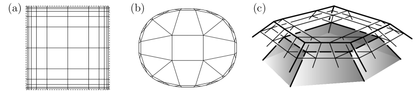
Figure 5.6: (a) A properly convex domain consisting only of squares. This example is uninteresting because it is a product of two properly convex domains. (b) A properly convex domain. It is a strictly residually convex $2$-complex and consists only of quadrilaterals. The union of any two adjacent quadrilaterals is a hexagon. (c) Using cubes and prisms, one can construct the stars $st^{k}(Q)$ of a simple polytope $Q$ so that the combinatorics of $st^{k}(Q)$ and $Q$ are the same.

Instead of considering those galleries starting from a fixed cell $Q$ in the direction of its facets, we could also consider galleries starting from facets in the boundary of a star $st^{k}(Q)$ for sufficiently large $k$. If the combinatorial complexity of the stars $st^{k}(Q)$ (viewed as polytopes) grows unlimitedly as $k$ increases, then so too does the chance that there are many distinct supporting hyperplanes associated to galleries starting from the facets in the boundary of $st^{k}(Q)$, so that we can always choose $n+1$ such in general position. Thus one may ask:

Question: Find conditions which guarantee that the combinatorial complexity of $st^{k}(Q)$ strictly increases as $k$ increases.

This question is interesting in view of the fact that properly convex real projective structures behave very similarly to metric spaces of non-positive curvature (see Section 6.1); answers to this question can possibly turn out to be restrictions on the fundamental domains and the gluing maps for such spaces. A number of reasonable approaches to this question are as follows:

(1) Figure 5.6 (b) motivates the following condition in addition to residual convexity: for each adjacent pair of $n$-cells $P_{1}$ with $k_{1}$ facets and $P_{2}$ with $k_{2}$ facets, we require that the underlying set of $P_{1}\cup P_{2}$ be an $n$-polytope with $k_{1}+k_{2}-2$ facets. In other words, we require that no two facets in the boundary of $P_{1}\cup P_{2}$ span a common hyperplane. We may call this property as strict residual convexity. In the case when the notion of angle makes sense, this condition amounts to not allowing right-angled polytopes.

Even when we do not require strict residual convexity, there are other possible answers to the above question.

(2) As we observed in Figure 1.2 (b) and (c), quadrilaterals are not good for our current purposes. Similar examples are also possible in general dimension with $n$-cubes taking the role of quadrilaterals, if $Q$ is a simple polytope. See Figure 5.6 (c). Even if we disallow $n$-cubes, however, by taking product with a $2$-dimensional example, we may obtain a complex consisting of $n$-prisms which is not properly convex. It seems that a complex without cubes and with a non-prism cell has good chance to be properly convex.

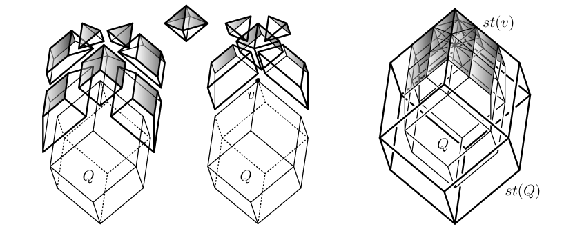
Figure 5.7: The $3$-polytope $Q$ and its star $st(Q)$ are rhombic dodecahedra. The star $st(v)$ of a non-simple vertex $v$ of $Q$ contains four pyramids.

(3) Suppose that $X$ contains an $n$-polytope $Q$ which has a non-simple vertex. Then it is very likely that the combinatorial complexity of $st^{k}(Q)$ strictly increases as $k$ increases: Figure 5.7 exhibits a way to construct the star $st(Q)$ of a rhombic dodecahedron $Q$ so that the combinatorics of $Q$ and $st(Q)$ are the same. The rhombic dodecahedron $Q$ has non-simple vertices. The star $st(v)$ of one of those non-simple vertices is shown in the picture. Observe that the star $st(v)$ contains four tetrahedra, which are prohibited in our current discussion because they are triangular. Moreover, the star $st(v)$ also contains some cubes. Thus it is very unlikely that one can construct the star $st(Q)$ of a non-simple polytope $Q$ without using triangular polytopes so that the combinatorics of $Q$ and $st(Q)$ are the same, even though cubes are allowed.

6 Applications to real projective structures

In this section we introduce real projective structures and prove Theorem A.

6.1 Convex real projective structures

Let $X$ be a smooth manifold and $G$ a Lie group acting on $X$. An $(X,G)$-structure on a manifold $M$ is a maximal atlas $\{(U_{i},\phi_{i})\}$ on $M$, where the family $\{U_{i}\}$ forms an open covering of $M$ and the maps $\phi_{i}:U_{i}\to X$ are coordinate charts such that the restriction of the transition map $\phi_{j}\circ\phi_{i}^{-1}$ to each component of $\phi_{i}(U_{i}\cap U_{j})$ is the restriction of an element of $G$. Let $M$ and $N$ be manifolds with $(X,G)$-structures. A map $f:M\to N$ is an $(X,G)$-map if, for each pair of charts $\phi_{i}:U_{i}\to X$ and $\psi_{j}:V_{j}\to X$ for $M$ and $N$, respectively, the restriction of the composition $\psi_{j}\circ f\circ\phi_{i}^{-1}$ to each component of $\phi_{i}(U_{i}\cap f^{-1}(V_{j}))$ is the restriction of an element of $G$.

Let $M$ be a manifold with $(X,G)$-structure. Let $p:\tilde{M}\to M$ be the universal covering space of $M$ and identify $\pi_{1}(M)$ with the group of covering transformations. Then there is a unique $(X,G)$-structure on $\tilde{M}$ for which $p$ is an $(X,G)$-map. Furthermore, the Development Theorem (see [7]) says that there exists a pair $(dev,\rho)$ where $dev:\tilde{M}\to X$ is an $(X,G)$-map and $\rho:\pi_{1}(M)\to G$ is a homomorphism such that

$$dev\circ\gamma=\rho(\gamma)\circ dev$$

for each $\gamma\in\pi_{1}(M)$. If $(dev^{\prime},\rho^{\prime})$ is another such pair, there exists $g\in G$ such that $dev^{\prime}=g\circ dev$ and $\rho^{\prime}(\gamma)=g\rho(\gamma)g^{-1}$ for each $\gamma\in\pi_{1}(M)$.

A real projective structure is an $(X,G)$-structure where $X$ is the real projective space $\mathbb{R}\textup{P}^{n}$ and $G$ is the group $\textup{Aut}(\mathbb{R}\textup{P}^{n})$ of projective automorphisms. The universal cover $\mathbb{S}^{n}$ of $\mathbb{R}\textup{P}^{n}$ is called the projective $n$-sphere and its group $\textup{Aut}(\mathbb{S}^{n})$ of projective automorphisms is isomorphic to the group $SL^{\pm}(n+1,\mathbb{R})$ of real matrices of determinant $\pm 1$. A real projective structure can also be defined as a $(\mathbb{S}^{n},\textup{Aut}(\mathbb{S}^{n}))$-structure (see [7, Exercise 4.5]). For the sake of convenience, we shall adopt the latter as our definition of real projective structures.

Let $M$ be a real projective $n$-manifold, that is, a manifold with a real projective structure. If the developing map

$$dev:\tilde{M}\to\mathbb{S}^{n}$$

is an embedding onto a convex (resp. properly convex) domain $\Omega\subset\mathbb{S}^{n}$ (see Section 2), then the structure on $M$ is said to be convex (resp. properly convex) and the manifold $M$ is called a convex (resp. properly convex) real projective manifold.

Convex real projective structures enjoy some nice properties, which we explain as follows. Let $M$ be a convex real projective $n$-manifold. Then $M$ is isomorphic to the quotient $\Omega/\Gamma$, where $\Omega\subset\mathbb{S}^{n}$ is a convex domain and $\Gamma\subset\textup{Aut}(\mathbb{S}^{n})$ is a discrete subgroup acting freely and properly discontinuously on $\Omega$. In particular, the fundamental group of $M$ is identified with $\Gamma$ and hence linear. Furthermore, because $\Omega$ is convex, the universal cover of $M$ is contractible and any two points $x$ and $y$ of $M$ can be connected by a line segment which is the projection of a line segment in $\Omega$ connecting a lift $\tilde{x}\in\Omega$ of $x$ to a lift $\tilde{y}\in\Omega$ of $y$. This property resembles the notion of geodesic completeness of Riemannian metrics. For this reason, convex real projective structures can be regarded as natural analogues of complete Riemannian metrics.

Properly convex real projective structures are expected to resemble non-positively curved metrics. For example, Benoist [1, 2] showed the followings: Let $M$ be a compact properly convex real projective $n$-manifold. As above, represent $M$ as the quotient $M=\Omega/\Gamma$, where $\Omega\subset\mathbb{S}^{n}$ is a properly convex domain and $\Gamma\subset\textup{Aut}(\mathbb{S}^{n})$ acts on $\Omega$ cocompactly. Then $\Omega$ is strictly convex if and only if $\Gamma$ is Gromov-hyperbolic. (Here, strict convexity of $\Omega$ means that the boundary $\partial\Omega$ does not contain any open line segment.) Furthermore, if $n=3$ and $\Omega$ is neither strictly convex nor reducible, then $M$ admits the JSJ-decomposition along embedded tori into hyperbolic pieces. In particular, such $M$ admits a Riemannian metric of non-positive curvature (see [14]).

6.2 Obtaining real projective manifolds

In this section, we present a version of the Poincaré fundamental polyhedron theorem for real projective structures, which will complement our main theorem in Section 6.3.

Let $\mathcal{P}$ be a finite family of $n$-polytopes in $\mathbb{S}^{n}$. Denote by $\Sigma$ the collection of all facets of the polytopes in $\mathcal{P}$. A projective facet-pairing for $\mathcal{P}$ is a set

$$\Phi=\{\phi_{\sigma}\in\textup{Aut}(\mathbb{S}^{n})\,|\,\sigma\in\Sigma\}$$

of elements of $\textup{Aut}(\mathbb{S}^{n})$ indexed by $\Sigma$ such that

• for each facet $\sigma$ of $P\in\mathcal{P}$ there is a facet $\sigma^{\prime}$ of $P^{\prime}\in\mathcal{P}$ such that $\phi_{\sigma}(\sigma)=\sigma^{\prime}$;

• the polytopes $\phi_{\sigma}(P)$ and $P^{\prime}$ are situated so that $\phi_{\sigma}(P)\cap P^{\prime}=\sigma^{\prime}$;

• the maps $\phi_{\sigma}$ and $\phi_{\sigma^{\prime}}$ satisfy the relation $\phi_{\sigma^{\prime}}=\phi_{\sigma}^{-1}$.

Let $\Phi$ be a projective facet-pairing for $\mathcal{P}$. Then $\Phi$ induces an equivalence relation on the disjoint union $\Pi=\bigsqcup_{P\in\mathcal{P}}P$. The corresponding quotient space $M$ of $\Pi$ is said to be obtained by gluing together the polytopes of $\mathcal{P}$ by $\Phi$. Let $M^{\prime}$ denote the space $M$ removed with its cells of codimension $\geq 2$. The space $M^{\prime}$ has a natural structure of a real projective orbifold, which is a manifold provided that $\phi_{\sigma}(\sigma)\neq\sigma$ for every facet $\sigma\in\Sigma$. While the following discussion has a straightforward generalization in the context of real projective orbifolds, we assume, for simplicity, that $M^{\prime}$ is a real projective manifold.

In what follows, we shall obtain a necessary condition for the real projective structure on $M^{\prime}$ to extends to $M$ and for the space $M$ to be a real projective manifold.

For this purpose, note first that the equivalence relation on $\Pi$ also induces an equivalence relation on the collection of ridges of the polytopes in $\mathcal{P}$. More precisely, let $e:=e_{1}$ be a ridge of $P_{1}\in\mathcal{P}$. Choose a facet $\sigma_{1}$ of $P_{1}$ containing $e_{1}$. Then there is a facet $\sigma_{1}^{\prime}$ of $P_{2}\in\mathcal{P}$ such that $\phi_{\sigma_{1}}(\sigma_{1})=\sigma_{1}^{\prime}$. Let $e_{2}=\phi_{\sigma_{1}}(e_{1})$ and let $\sigma_{2}$ be the facet of $P_{2}$ other than $\sigma_{1}^{\prime}$ which contains $e_{2}$. Then there is a facet $\sigma_{2}^{\prime}$ of $P_{3}\in\mathcal{P}$ such that $\phi_{\sigma_{2}}(\sigma_{2})=\sigma_{2}^{\prime}$. Continuing in this manner, we obtain a sequence $\{e_{i}\}$ of ridges, a sequence $\{P_{i}\}$ of polytopes, a sequence $\{\phi_{\sigma_{i}}\}$ of facet-pairing transformations, and a sequence $\{\sigma_{i},\sigma_{i}^{\prime}\}$ of pairs of facets. Because the family $\mathcal{P}$ is finite and there are only finitely many ridges in a polytope, the sequence of ridges is periodic and hence all four sequences are periodic. Let $r$ be the least common period of these four sequences. Note that the period $r$, as well as the two conditions we shall consider below, are independent of our choice above between $\sigma_{1}$ and $\sigma_{1}^{\prime}$.

We set $h(e)=\phi_{\sigma_{r}}\circ\cdots\circ\phi_{\sigma_{1}}$ and consider the following sequence of polytopes in $\mathbb{S}^{n}$

$$P_{1},\;\phi_{\sigma_{1}}^{-1}(P_{2}),\;\phi_{\sigma_{1}}^{-1}\phi_{\sigma_{2}}^{-1}(P_{3}),\;\cdots,\phi_{\sigma_{1}}^{-1}\phi_{\sigma_{2}}^{-1}\cdots\phi_{\sigma_{r-1}}^{-1}(P_{r}).$$

Observe that all polytopes in the sequence share the ridge $e$ in common and each successive polytopes are adjacent. Thus, if we put the standard Riemannian metric on $\mathbb{S}^{n}$ and consider the link $\textup{Lk}(e;P)$ for each polytope $P$ in the above sequence, then we obtain a sequence $\{\alpha_{i}\}$ of segments in $\mathbb{S}^{1}=L(e)^{\bot}\subset\mathbb{S}^{n}$. Let $\textup{Lk}(e)=(\alpha_{1}\sqcup\cdots\sqcup\alpha_{r})/_{\sim}$ denote the natural identification space of these segments.

Now, for the space $M$ to be a real projective manifold, it is necessary that, for each ridge $e$, we have $h(e)=id$ and the isometry $L(e)=\mathbb{S}^{1}$. It turns out that these conditions are also sufficient. The proof of the following proposition is analogous to the usual proofs of the Poincaré fundamental polyhedron theorem for constant curvature Riemannian metrics (see, for example, [5] and [15]) and we omit it.

Proposition 6.1.

Let $\mathcal{P}$ be a finite family of $n$-polytopes in $\mathbb{S}^{n}$. Let $\Phi$ be a projective facet-pairing for $\mathcal{P}$. Let $M$ be the space obtained by gluing together the polytopes of $\mathcal{P}$ by $\Phi$. Then $M$ is a real projective manifold provided that, for each ridge $e$ of a polytope in $\mathcal{P}$, we have

1. $h(e)=id$;

2. $\textup{Lk}(e)$ is isometric to the unit circle $\mathbb{S}^{1}$.

6.3 Convexity theorem for real projective structures

We are now ready to prove Theorem A. To apply the results obtained in Section 4 and Section 5 more conveniently, however, we prove the following equivalent theorem which is stated in terms of $(\mathbb{S}^{n},\textup{Aut}(\mathbb{S}^{n}))$-structures.

Theorem 6.2.

Let $\mathcal{P}$ be a finite family of $n$-polytopes in the projective $n$-sphere $\mathbb{S}^{n}$. Let $\Phi=\{\phi_{\sigma}\in\textup{Aut}(\mathbb{S}^{n})\,|\,\sigma\in\Sigma\}$ be a projective facet-pairing for $\mathcal{P}$, where $\Sigma$ is the collection of all facets of the polytopes in $\mathcal{P}$. Let $M$ be a real projective $n$-manifold obtained by gluing together the polytopes in $\mathcal{P}$ by $\Phi$. Assume the following condition:

for each facet $\sigma$ of $P\in\mathcal{P}$, if $\sigma^{\prime}$ is a facet of $P^{\prime}\in\mathcal{P}$ such that $\phi_{\sigma}(\sigma)=\sigma^{\prime}$, then the union $\phi_{\sigma}(P)\cup P^{\prime}$ is a convex subset of $\mathbb{S}^{n}$.

Then the following assertions are true:

1. If $\mathcal{P}$ contains no triangular polytope, then $M$ is a convex real projective manifold;

2. If, in addition, $\mathcal{P}$ contains a polytope $P$ whose dual $P^{*}$ is thick, then $M$ is a properly convex real projective manifold.

Proof.

Let $dev:\tilde{M}\to\mathbb{S}^{n}$ be the associated developing map of the universal covering space $\tilde{M}$ of $M$. Regard the projective sphere $\mathbb{S}^{n}$ as the standard Riemannian sphere and pullback the Riemannian metric to $\tilde{M}$ via $dev$. Then the above condition on the facet-pairing for $\mathcal{P}$ and the assumption that $M$ is a real projective $n$-manifold, imply that $\tilde{M}$ is a residually convex $n$-complex (as defined in Definition 3.1 and Definition 4.2). Now the conclusions of the theorem follow immediately from Corollary 4.13 and Theorem 5.1. ∎

Remark 6.3.

(1) It is not difficult to see that an orbifold version of Theorem 6.2 is also true.

(2) Let $P\subset\mathbb{S}^{n}$ be an $n$-polyhedron (which is not necessarily a polytope). Suppose that $\Gamma\subset\textup{Aut}(\mathbb{S}^{n})$ is a group generated by (projective) reflections in the hyperplanes spanned by facets of $P$. In [16] Vinberg provided necessary and sufficient conditions for $\Gamma$ to be a discrete subgroup with fundamental domain $P$. In such case, he also showed that the orbit $\Gamma(P)\subset\mathbb{S}^{n}$ of $P$ under $\Gamma$ is a convex subset and $\Gamma$ acts properly discontinuously on the interior $\Omega$ of $\Gamma(P)$.

It is easy to see that gluing by reflections necessarily gives rise to residually convex structures. Thus, in some special cases, our result provides another proof that the domain $\Omega$ above is convex. Namely, if $P$ is a non-triangular $n$-polytope, if $\Gamma$ is known to be discrete, and if all stabilizer subgroups of points of $P$ are finite, then $\Gamma(P)=\Omega$ is a residually convex $n$-complex without triangular polytopes and hence Corollary 4.13 applies.

On the other hand, because our gluing maps are not necessarily reflections, our results do cover complementary part of Vinberg’s convexity assertion. For instance, it is well-known that cocompact/cofinite hyperbolic reflection groups are non-existent in higher dimensions. More generally, a similar non-existence assertion is also true for cocompact (projective) reflection groups acting on strictly convex domains (see [9]).

(3) In his paper [11], after producing real projective structures on Gromov-Thurston manifolds, Kapovich showed that these structures are in fact convex. There he deals with polyhedral complexes which are similar to our residually convex $n$-complexes. But, because the polyhedra he considers have infinitely many facets, his complexes are assumed to satisfy more properties than residual convexity and are rather complicated to describe. His proof modifies Vinberg’s arguments and applies small cancelation theory to the $2$-skeleton of the dual complexes.

Department of Mathematics,

University of California,

Davis, CA 95616, USA,

zlee@math.ucdavis.edu

References

- [1] Y. Benoist, Convexes divisibles. I, in Algebraic groups and arithmetic, Tata Inst. Fund. Res., Mumbai, 2004, pp. 339–374.
- [2] , Convexes divisibles. IV. Structure du bord en dimension 3, Invent. Math., 164 (2006), pp. 249–278.
- [3] M. R. Bridson and A. Haefliger, Metric spaces of non-positive curvature, vol. 319 of Grundlehren der Mathematischen Wissenschaften, Springer-Verlag, Berlin, 1999.
- [4] Y. Burago, M. Gromov, and G. Perelman, A. D. Aleksandrov spaces with curvatures bounded below, Uspekhi Mat. Nauk, 47 (1992), pp. 3–51, 222.
- [5] D. B. A. Epstein and C. Petronio, An exposition of Poincaré’s polyhedron theorem, Enseign. Math. (2), 40 (1994), pp. 113–170.
- [6] W. Fenchel, Convex cones, sets, and functions. Mimeographed lecture notes, 1953.
- [7] W. M. Goldman, Projective geometry on manifolds. Lecture notes, 1988.
- [8] B. Grünbaum, Convex polytopes, vol. 221 of Graduate Texts in Mathematics, Springer-Verlag, New York, second ed., 2003.
- [9] T. Januszkiewicz and J. Światkowski, Hyperbolic Coxeter groups of large dimension, Comment. Math. Helv., 78 (2003), pp. 555–583.
- [10] , Simplicial nonpositive curvature, Publ. Math. Inst. Hautes Études Sci., (2006), pp. 1–85.
- [11] M. Kapovich, Convex projective structures on Gromov–Thurston manifolds. (to appear in Geometry and Topology).
- [12] J. Lee, Convex fundamental domains for properly convex real projective structures. (in preparation).
- [13] , On thin simple -dimensional polytopes. (in preparation).
- [14] B. Leeb, -manifolds with(out) metrics of nonpositive curvature, Invent. Math., 122 (1995), pp. 277–289.
- [15] J. G. Ratcliffe, Foundations of hyperbolic manifolds, vol. 149 of Graduate Texts in Mathematics, Springer-Verlag, New York, 1994.
- [16] È. B. Vinberg, Discrete linear groups that are generated by reflections, Izv. Akad. Nauk SSSR Ser. Mat., 35 (1971), pp. 1072–1112.