Ly Emission-Line Galaxies at in the Extended Chandra Deep Field South
Abstract
We describe the results of an extremely deep, 0.28 deg2 survey for Ly emission-line galaxies in the Extended Chandra Deep Field South. By using a narrow-band 5000 Å filter and complementary broadband photometry from the MUSYC survey, we identify a statistically complete sample of 162 galaxies with monochromatic fluxes brighter than ergs cm-2 s-1 and observers frame equivalent widths greater than 80 Å. We show that the equivalent width distribution of these objects follows an exponential with a rest-frame scale length of Å. In addition, we show that in the emission line, the luminosity function of Ly galaxies has a faint-end power-law slope of , a bright-end cutoff of , and a space density above our detection thresholds of galaxies Mpc-3. Finally, by comparing the emission-line and continuum properties of the LAEs, we show that the star-formation rates derived from Ly are times lower than those inferred from the rest-frame UV continuum. We use this offset to deduce the existence of a small amount of internal extinction within the host galaxies. This extinction, coupled with the lack of extremely-high equivalent width emitters, argues that these galaxies are not primordial Pop III objects, though they are young and relatively chemically unevolved.
1 Introduction
The past decade has seen an explosion in our ability to detect and study galaxies and probe the history of star formation in the universe (e.g., Madau et al., 1996). This has been mostly due to the development of the Lyman-break technique, whereby high redshift galaxies are identified via a flux discontinuity caused by Lyman-limit absorption (see Steidel et al., 1996a, b). By taking deep broadband images, and searching for , , and -band dropouts, astronomers have been able to explore large-scale structure and determine the properties of bright () galaxies between and (Giavalisco, 2002).
The stunning success of the Lyman-break technique stands in contrast to the initial results of Ly emission-line observations. The failure of the first generation of these surveys (e.g., De Propis et al., 1993; Thompson, Djorgovski, & Trauger, 1995) was attributed to internal extinction in the target galaxies (Meier & Terlevich, 1981). Since Ly photons are resonantly scattered by interstellar hydrogen, even a small amount of dust can reduce the emergent emission-line flux by several orders of magnitude.
Fortunately, Ly surveys have recently undergone a resurgence. Starting with the Keck observations of Cowie & Hu (1998) and Hu, Cowie, & McMahon (1998), narrow-band searches for Ly emission have been successfully conducted at a number of redshifts, including (Stiavelli et al., 2001), (Ciardullo et al., 2002; Hayashino et al., 2004; Venemans et al., 2005; Gawiser et al., 2006a), (Fujita et al., 2003), (Rhoads et al., 2000), (Ouchi et al., 2003), (Rhoads et al., 2003; Ajiki et al., 2003; Tapken et al., 2006), and (Kodaira et al., 2003; Taniguchi et al., 2005). The discovery of these high-redshift Ly emitters (LAEs) has opened up a new frontier in astronomy. At , LAEs are as easy to detect than Lyman-break galaxies (LBG), and, by , they are the only galaxies observable from the ground. By selecting galaxies via their Ly emission, it is therefore possible to probe much further down the galaxy continuum luminosity function than with the Lyman-break technique, and perhaps identify the most dust-free objects in the universe. In addition, by using Ly emitters as tracers of large-scale structure (Steidel et al., 2000; Shimasaku et al., 2004), it is possible to efficiently probe the expansion history of the universe with a minimum of cosmological assumptions (e.g., Blake & Glazebrook, 2003; Seo & Eisenstein, 2003; Koehler et al., 2007).
Here, we describe the results of a deep survey for Ly emission-line galaxies in a 0.28 deg2 region centered on the Extended Chandra Deep Field South (ECDF-S). This region has an extraordinary amount of complementary data, including high-resolution optical images from the Hubble Space Telescope via the Great Observatories Origins Deep Survey (GOODS; Giavalisco et al., 2004) and the Galaxy Evolution from Morphology and SEDs program (GEMS; Rix et al., 2004), deep groundbased photometry from the Multiwavelength Survey by Yale-Chile (MUSYC; Gawiser et al., 2006b), mid- and far-IR observations from Spitzer, GOODS and MUSYC, and deep X-ray data from Chandra (Giacconi et al., 2002; Alexander et al., 2003; Lehmer et al., 2005). In Section 2, we describe our observations, which include over 28 hours worth of exposures through a narrow-band filter on the CTIO 4-m telescope. We also review the techniques used to detect the emission-line galaxies, and discuss the difficulties associated with analyzing samples of LAEs discovered via fast-beam instruments. In Section 3, we describe the continuum properties of our Ly emitters, including their rest-frame colors, and compare their space density to that of Lyman-break galaxies. In Section 4, we examine the LAE’s equivalent width distribution and show that our sample contains very few of the extremely-high equivalent width objects found by Dawson et al. (2004) at . In Section 5, we present the Ly emission-line luminosity function, and give values for its best-fit Schechter (1976) parameters and normalization. In Section 6, we translate these Ly fluxes into star-formation rates, and consider the properties of LAEs in the context of the star-formation rate (SFR) history of the universe. We conclude by discussing the implications our observations have for surveys aimed at determining cosmic evolution.
For our analysis, we adopt a CDM cosmology with km s-1 Mpc-1 (), , and . At , this implies a physical scale of 7.6 kpc per arcsecond.
2 Observations and Reductions
Narrow-band observations of the ECDF-S were performed with the MOSAIC II CCD camera on the CTIO Blanco 4-m telescope. These data consisted of a series of 111 exposures taken over 16 nights through a 50 Å wide full-width-half-maximum (FWHM) filter (see Figure 1). The total exposure time for these images was 28.17 hr; when the effects of dithering to cover for a dead CCD during some of the observations are included, the net exposure time becomes hr. The total area covered in our survey is 998 arcmin2; after the regions around bright stars are excluded, this area shrinks 993 arcmin2. The overall seeing on the images is . A log of our narrow-band exposures appears in Table 1.
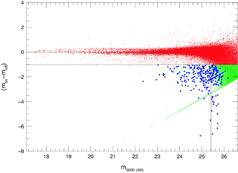
The procedures used to reduce the data, identify line emitters, and measure their brightnesses were identical to those detailed in Ciardullo et al. (2002) and Feldmeier et al. (2003). After de-biasing, flat-fielding, and aligning the data, our narrow-band frames were co-added to create a master image that was clipped of cosmic rays. This frame was then compared to a deep + continuum image provided by the MUSYC survey (Gawiser et al., 2006b) in two different ways. First, the DAOFIND task within IRAF was run on the summed narrow-band and continuum image using a series of three convolution kernels, ranging from one matching the image point-spread-function (PSF), to one times larger. This created a source catalog of all objects in our field. These targets were then photometrically measured with DAOPHOT’s PHOT routine, and sources with on-band minus continuum colors less than in the AB system were flagged as possible emission-line sources (see Figure 2). At the same time, candidate LAEs were also identified by searching for positive residuals on a “difference” image made by subtracting a scaled version of the + continuum image from the narrow-band frame. In this case, the DAOFIND algorithm was set to flag all objects brighter than four times the local standard deviation of the background sky (see Figure 3). As pointed out by Feldmeier et al. (2003), these two techniques complement each other, since each detects objects that the other does not. Specifically, of galaxies were missed by the color-magnitude method due to image blending and confusion, but found with the difference method. Conversely, objects at the frame limit that were lost amidst the increased noise of the difference frame, could still be identified via their on-band minus off-band colors.
Finally, because we intentionally biased our DAOFIND parameters to identify faint sources at the expense of false detections, each emission-line candidate was visually inspected on the narrow-band, continuum, and difference frames, as well as two frames made from subsamples of half the on-band exposures. This last step excluded many false detections at the frame limit, and left us with a sample of 259 candidate LAEs for analysis.
Once found, the equatorial positions of the candidate emission-line galaxies were derived with respect to the reference stars of the USNO-A 2.0 astrometric catalog (Monet et al., 1998). The measured residuals of the plate solution were , a number slightly less than the external error associated with the catalog. Relative narrow-band magnitudes for the objects were derived by first measuring the sources with respect to field stars using an aperture slightly greater than the frame PSF. Since most of the galaxies detected in this survey are, at best, marginally resolved on our images, this procedure was sufficiently accurate for our purposes. We then obtained standard AB magnitudes by comparing large aperture photometry of the field stars to similar measurements of the spectrophotometric standards Feige 56 and Hiltner 600 (Stone, 1977) taken on three separate nights. The dispersion in the photometric zero point computed from our standard star measurements was 0.03 mag.
2.1 Derivation of Monochromatic Fluxes
The fast optics of wide-field instruments, such as the MOSAIC camera at the CTIO 4-m telescope, present an especially difficult challenge for narrow-band imaging. The transmission of an interference filter depends critically on the angle at which it is illuminated: light entering at the normal will constructively/destructively interfere at a different wavelength than light coming in at an angle (Eather & Reasoner, 1969). As a result, when placed in a fast converging beam, an interference filter will have its bandpass broadened and its peak transmission decreased by a substantial amount. This effect is important, for without precise knowledge of the filter bandpass, it is impossible to derive accurate monochromatic fluxes or estimate equivalent widths.
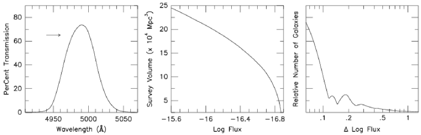
To derive the filter transmission, we began with the throughput information provided by the CTIO observatory111http://www.ctio.noao.edu/instruments/FILTERS/index.html. This curve, which represents the expected transmission of the [O III] interference filter in the f/3.2 beam of the Blanco telescope, was computed by combining laboratory measurements of the filter tipped at several different angles from the incoming beam (for a discussion of this procedure, see Jacoby et al., 1989). We then shifted this curve 2 Å to the blue, to compensate for the thermal contraction of the glass at the telescope, and compared this model bandpass to the measured emission-line wavelengths obtained from follow-up spectroscopy (Lira et al., 2007). Interestingly, redshift measurements of 72 galaxies detected in three independent MUSYC fields confirm the shape of the filter’s transmission curve, but not its central wavelength: according to the spectroscopy, the mean wavelength of the filter is 10 Å bluer than given by CTIO (Gawiser et al., 2007). Examining the source of this discrepancy is beyond the scope of this paper. However, the data do confirm that, when placed in the beam of the CTIO 4-m prime focus MOSAIC camera, the bandpass of the CTIO [O III] interference filter is nearly Gaussian in shape. This bandpass is reproduced in the left-hand panel of Figure 4.
This non-square bandpass has important consequences for the analysis of large samples of emission-line galaxies. The first of these involves the definition of survey volume. Because the transmission of the filter declines away from the bandpass center, the volume of space sampled by our observations is a strong function of line strength. This is illustrated in the center panel of Figure 4. Objects with bright line emission can be detected even if their redshifts place Ly in the wings of the filter, hence the volume covered for these objects is realtively large. Conversely, weak Ly sources must have their line emission near the center of the bandpass to be observable. As a result, the “effective” volume for our integrated sample of galaxies is a function of the galaxy emission-line luminosity function.
A second concern deals with the sample’s flux calibration. In order to compare the flux of an emission-line object to that of a spectrophotometric standard star (i.e., a continuum source) one needs to know both the filter’s integral transmission and its monochromatic transmission at the wavelength of interest (Jacoby et al., 1987, 1989). When observing objects at known redshift, the latter requirement is not an issue. However, when measuring a set of galaxies which can fall anywhere within a Gaussian-shaped transmission curve, the transformation between an objects’ (bandpass-dependent) AB magnitude and its monochromatic flux is not unique. In fact, if we assume that galaxies are (on average) distributed uniformly in redshift space, then the number of emission-line objects present at a given transmission, , is simply proportional to the amount of wavelength associated with that transmission value. Consequently, the observed distribution of emission-line fluxes will be related to the true distribution via a convolution, whose (unity normalized) kernel, , is
| (1) |
where the first term describes the filter’s response blueward of the transmission peak and the second term gives the response redward of the peak. The center panel of Figure 4 displays this kernel for the filter used in our survey. The curve shows that for roughly half of the detectable galaxies in our field, the effect of our filter’s non-square bandpass is minimal. However, for the other of galaxies, the shape of the bandpass is extremely important, and the inferred fluxes for some objects can be off by over a magnitude.
Any analysis of the ensemble properties of our LAEs must consider the full effect that the non-square bandpass and the odd-shaped convolution kernal has on the sample. We do this in Sections 4 and 5. However, one often wants to quote the monochromatic flux and equivalent width for an individual Ly emitter. To do this, we need to adopt an appropriate “mean” value for the transmission of our filter. The most straightforward way to define this number is via the filter’s peak transmission. This is where the survey depth is greatest, and choosing is equivalent to assigning each galaxy its “most probable” monochromatic flux. Unfortunately, by defining the transmission in this way, we underestimate the flux from all galaxies whose line emission does not fall exactly on this peak. Alternatively, we can attempt to choose a transmission which globally minimizes the flux errors of all the galaxies detected in the survey. This can be done by weighting each transmission by the number of galaxies one expects to observe at that wavelength: the greater the transmission, the deeper the survey, and the more galaxies present in the sample. The difficulty with this “expectation value” approach is that it requires prior knowledge of the distribution of emission-line fluxes, which is one of the quantities we are attempting to measure. That leads us to a third possibility: to approximate the filter’s expectation value using some “characteristic” transmission, , which is independent of the galaxy luminosity function, but still takes the filter’s changing transmission into account. The arrow in Figure 4 identifies the transmission we selected as being characteristic of the filter; the justification for this value is presented in Section 5. We emphasize that is only a convenient mean that enables us to quote the likely emission-line strengths of individual galaxies. When analyzing the global properties of an ensemble of LAEs, the full non-Gaussian nature of the filter’s convolution kernel must be taken into account.
Using this transmission and our knowledge of the filter curve, we converted the galaxies’ AB magnitudes to monochromatic fluxes at Å via
| (2) |
where is given in ergs cm-2 s-1 (Jacoby et al., 1987). Equivalent widths then followed via
| (3) |
where is the objects’ AB flux density in the continuum image, and , the FWHM of the narrow-band filter, represents the contribution of the galaxy’s underlying continuum within the bandpass. Both these equations are only applicable to objects whose line emission dominates the continuum within the narrow-band filter’s bandpass. Since we are limiting our discussion to galaxies with narrow-band minus broad-band AB magnitudes more negative than , this approximation is certainly valid. However, we do note that by using instead of , we are intentionally overestimating the flux and equivalent width of some galaxies, in order to minimize the errors in others. So, while the application of formally translates our criterion into a minimum emission-line equivalent width of 90 Å, galaxies with emission-lines that fall near the peak of the filter transmission function can have equivalent widths that are smaller. This implies that the absolute minimum equivalent width limit for our sample of LAEs is 80 Å.
2.2 Sample of LAE Candidates
Tables 2 and 3 give the coordinates of each candidate emission-line galaxy, along with its inferred monochromatic flux and equivalent width. In total, 259 objects are listed, though many are beyond the limit of our completeness. To determine this limit, we followed the procedures of Feldmeier et al. (2003) and added 1,000,000 artificial stars (2000 at a time) to our narrow-band frame. By re-running our detection algorithms on these modified frames, we were able to compute the flux level below which the object recovery fraction dropped below the 90% threshold. This value, which corresponds to a monochromatic flux of ergs cm-2 s-1 () is our limiting magnitude for statistical completeness; 162 galaxies satisfy this criterion.
Before proceeding further with our analysis, we performed one additional check on our data. To eliminate obvious AGN from our sample, we cross-correlated our catalog of emission-line objects with the lists of X-ray sources found in the 1 Msec exposure of the Chandra Deep Field South (Alexander et al., 2003), and the four 250 ksec exposure of the Extended Chandra Deep Field South (Lehmer et al., 2005; Virani et al., 2006). Two of our LAE candidates were detected in the X-ray band. The first, which is our brightest Ly emitter, has a 0.5 – 8 keV flux of ergs cm-2 s-1 (i.e., ergs s-1 at ) and exhibits C IV emission at 1550 Å (Lira et al., 2007). The other is an interloper: a AGN detected via its strong C III] line at 1909 Å. For the remaining 160 objects that were not detected individually in the X-ray band, we used stacking analyses to constrain their mean X-ray power output (see Lehmer et al., 2007, for details). We find that the stacked X-ray signal, which corresponds to a ksec effective exposure on an average LAE, does not yield a detection in any of three X-ray bandpasses (0.5–8.0 keV, 0.5–2.0 keV, and 2–8 keV). These results imply a upper-limit of ergs s-1 on the mean 0.5–2.0 keV luminosity for our LAEs, which demonstrates that few of our Ly sources harbor low-luminosity AGN. Similarly, if we use the conversion of Ranalli et al. (2003), we can translate this X-ray non-detection into an upper-limit for a typical LAE’s star-formation rate. This limit, yr-1, is roughly an order of magnitude greater than the rates inferred from the objects’ Ly emission or UV continua (see Section 6).
For the remainder of this paper, we will treat our X-ray source as AGN and exclude it from the analysis. This leaves us with a sample of 160 objects, which we assume are all star-forming galaxies. We note that, because all of our objects have equivalent widths greater than 80 Å, they are unlikely to be [O II] emitters. At , our survey volume is only Mpc3, which, through the luminosity functions of Hogg et al. (1998), Gallego et al. (2002), and Teplitz et al. (2003), implies a total population of between and [O II] emission-line galaxies above our completeness limit. Since less than 2% of these objects will have rest frame equivalent widths greater than Å (Hogg et al., 1998), the number of [O II] interlopers in our sample should be negligible. This estimate is confirmed by follow-up spectroscopy: of the 52 LAE candidates observed with sufficient signal-to-noise for a redshift determination, all are confirmed Ly emitters (Gawiser et al., 2006a; Lira et al., 2007).
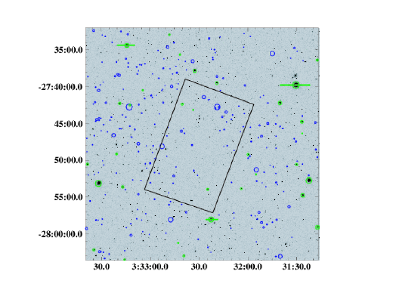
Figure 5 shows the spatial distribution of the LAEs above our completeness limit. The sources are obviously clustered, falling along what appear to be “walls” or “filaments”. The GOODS region has a below-average number of Ly emitters, and there are almost no objects in the northwestern part of the field. Conversely, the density of LAEs east and northeast of the field center is quite high. This type of data can be an extremely powerful probe of cosmological history, but we will defer a discussion of this topic to a future paper (Gawiser et al., 2007).
3 The Continuum Properties of the Emitters
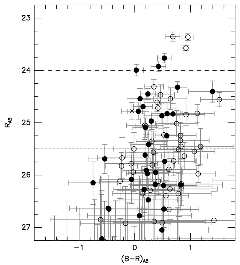
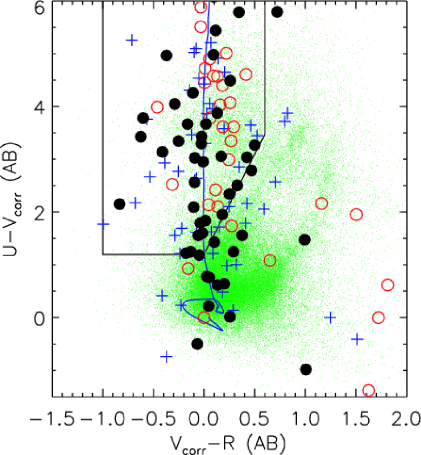
To investigate the continuum properties of our Ly emitters, we measured the brightness of each LAE on the broadband UBVR images of the MUSYC survey (Gawiser et al., 2006b). Since the catalog associated with this dataset has a detection threshold of , , , and , our knowledge of the LAEs’ positions (obtained from the narrow-band frames) allows us to perform photometry well past this limit. Figure 6 displays the color-magnitude diagram for 88 of the LAEs brighter than . The diagram, which shows the galaxies’ rest-frame continua at 1060 and 1570 Å, has several features of note.
The first involves the color distribution of our objects. According to the figure, LAEs with -band magnitudes brighter than have a median color of . This value agrees with the blue colors found by Venemans et al. (2005) for a sample of Ly emitters at , and is the value expected for a yr old stellar system evolving with a constant star-formation rate (Fujita et al., 2003; Bruzual & Charlot, 2003). This median color is also consistent with the results of Gawiser et al. (2006a), who stacked the broad-band fluxes of 18 spectroscopically confirmed LAEs and showed that the typical age of these systems is between Gyr. It does, however, stand in marked contrast to the results of Stiavelli et al. (2001), who claimed that Ly emitters at are very red (). The blue colors of our galaxies confirm their nature as young, star-forming systems. There is no evidence for excessive reddening in these objects, and if the galaxies do possess an underlying population of older stars, the component must be quite small.
On the other hand, as the LAE color distribution indicates, Ly emitters are not, as a class, homogeneous. At , the MUSYC colors have a typical photometric uncertainty of mag. This contrasts with the observed color dispersion for our galaxies, which is mag for objects with . Thus, there is at least a mag scatter in the intrinsic colors of these objects. Either there is some variation in the star-formation history of Ly emitters, or dust is having an effect on the emergent colors.
Finally, it is worth emphasizing that our Ly emitters are substantially fainter in the continuum than objects found by the Lyman-break technique. At , galaxies have an apparent magnitude of (Steidel et al., 1999) and ground-based Lyman-break surveys typically extend only mag beyond this value (see Giavalisco, 2002, for a review). Furthermore, spectroscopic surveys of LBG candidates rarely target galaxies fainter than . In our emission-line sample, the median continuum magnitude is , and many of the galaxies have aperture magnitudes significantly fainter than . In general, LAEs do inhabit the same location as LBGs in the - vs. - color-color space (see Figure 7), but their extremely faint continuum sets them apart.
This is also illustrated in Figure 8, which compares the rest frame 1570 Å luminosity function of our complete sample of Ly emitters (those with monochromatic fluxes greater than ergs cm-2 s-1) with the rest-frame 1700 Å luminosity function of Lyman-break galaxies (Steidel et al., 1999). When plotted in this way, our sample of LAEs appears incomplete, since for , only the brightest emission-line sources will make it into our catalog. The plot also implies that at , , Ly emitters are times rarer than comparably bright Lyman-break galaxies. Since this ratio is virtually identical to that measured by Steidel et al. (2000) within an extremely rich protocluster, this suggests that the number is not a strong function of galactic environment. But, most strikingly, our observations demonstrate the Ly emitters sample the entire range of the (UV-continuum) luminosity function. The median UV luminosity of LAEs in our sample is , and the faintest galaxy in the group is no brighter than . Just as broadband observations detect all objects at the bright-end of the continuum luminosity function, but sample the entire range of emission-line strengths, our narrow-band survey finds all the brightest emission-line objects, but draws from the entire range of continuum brightness.
4 The Ly Equivalent Width Distribution
Before examining the emission-line properties of our dataset, we need to correct for the observational biases and selection effects that are present in the sample. Since the data were taken in a fast-beam through a filter with a non-square bandpass, these effects are substantial. Continuum measurements, of course, are unaffected by the peculiarities of a narrow-band filter, but the distribution of monochromatic fluxes can be significantly distorted. Specifically, the observed flux distribution will be the convolution of the true distribution with the following two kernels:
The Photometric Error Function: The random errors associated with our narrow-band photometry vary considerably, ranging from mag at the bright end, to mag near the completeness limit (see Table 4). These errors will scatter objects from heavily populated magnitude bins into bins with fewer objects, and flatten the slope of the luminosity function. Because the change in slope goes as the square of the measurement uncertainty (Eddington, 1913, 1940), the effect of this convolution is most important for objects near the survey limit.
The Filter Transmission Function. As described in Section 2.1, the narrow-band filter used for this survey has a transmission function that is nearly Gaussian in shape. This creates an odd-shaped convolution kernel (the right panel of Figure 4), which systematically decreases the measured line-emission of objects falling away from the peak of the transmission curve. Moreover, because the objects’ equivalent widths are also reduced by this bandpass effect, some fraction of the LAE population will be lost from our EW Å sample. The result is that the normalization of this filter transmission kernel is not unity. Instead, it depends on the intrinsic equivalent width distribution of the galaxies, since that is the function that defines the fraction of galaxies (at each redshift) which can still make it into our sample.
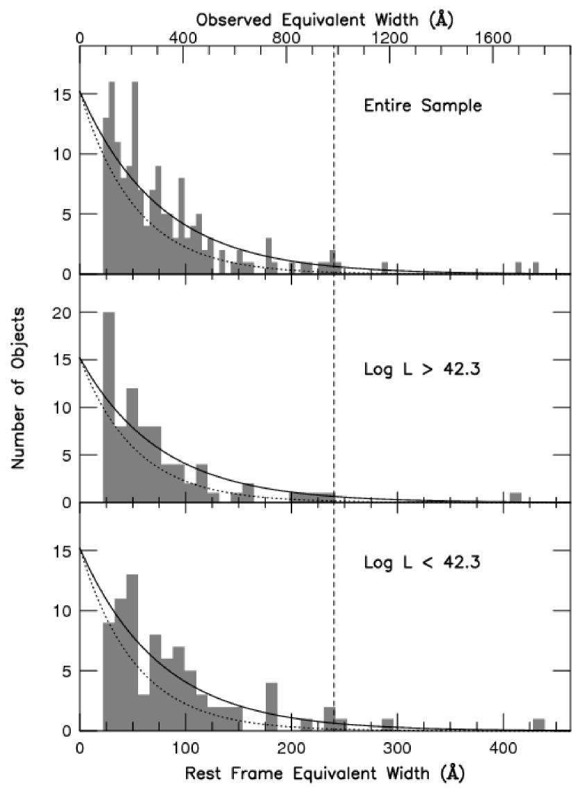
These effects are illustrated in the top panel of Figure 9, which displays a histogram of the rest-frame equivalent widths for our candidate Ly galaxies. As the dotted line shows, the data appear to be well fit by an exponential that has an e-folding length of Å. However, because the bandpass of our narrow-band filter is more Gaussian-shaped than square, the line-strengths of many of the galaxies have been systematically underestimated. In fact, the true distribution of equivalent widths is broader than that measured: when we perform a maximum-likelihood analysis using a series of exponential laws, convolved with the filter bandpass and photometric error kernels, we obtain a most-likely scale length of Å, or Å in the rest frame of the sample.
Such a distribution is quite different from that reported by Malhotra & Rhoads (2002). In their survey of 150 Ly emitters, of the objects had extremely high rest-frame equivalent widths, i.e., EW Å. Since stellar population models, such as those by Charlot & Fall (1993) cannot produce such strong line-emission, Malhotra & Rhoads (2002) postulated the presence of a top-heavy initial mass function and perhaps the existence of Population III stars. However in our sample, only 3 out of 160 LAEs () have observed rest-frame equivalent widths greater than this 240 Å limit. Even when we correct for the effects of our filter’s non-square bandpass, the fraction of strong line-emitters does not exceed . This is less than the value estimated by Dawson et al. (2004) via Keck spectroscopy of a subset of Malhotra & Rhoads (2002) objects. Thus, at least at , there is no need to invoke a skewed initial mass function to explain the majority of our LAEs.
The equivalent width distribution of Figure 9 also differs dramatically from that found by Shapley et al. (2003) for a sample of Lyman-break galaxies. In their dataset, rest-frame equivalent widths e-fold with a scale-length of Å, rather than the Å value derived from our LAE survey. This difference is not surprising given that the former dataset is selected to be bright in the continuum, while the latter is chosen to be strong in the emission-line. Moreover, when Shapley et al. (2003) analyzed the of Lyman-break galaxies with rest-frame equivalent widths greater than 20 Å, they found a correlation between line strength and continuum (-band) magnitude, in the sense that fainter galaxies had higher equivalent widths. We see that same trend in our data, but it is largely the result of a selection effect. (Faint galaxies with low equivalent widths fall below our monochromatic flux limit.) A comparison of emission-line flux with equivalent width for our statistically complete sample shows no such correlation.
The lower two panels of Figure 9 demonstrate this another way. In the diagram, our sample of LAEs is divided in half, with the middle panel showing the equivalent width distribution for objects with monochromatic Ly luminosities greater ergs s-1, and the bottom panel displaying the same distribution for less luminous objects. As the figure illustrates, the distribution of equivalent widths is relatively insensitive to the absolute brightness of the galaxy. To first order this is expected, since both the UV continuum and the Ly emission-line flux are driven by star formation. However, one could imagine a scenario wherein the amount, composition, and/or distribution of dust within the brighter (presumably more-metal rich) Ly emitters differs from that within their lower-luminosity counterparts. Since the effect of this dust on resonantly-scattered Ly photons is likely to be different from that on continuum photons, this change in extinction can theoretically produce a systematic shift in the distribution of Ly equivalent widths. There is no evidence for such a shift in our data; this constancy argues against the importance of dust in these objects.
5 The Ly Emission-Line Luminosity Function
Figure 10 shows the distribution of monochromatic fluxes for our sample of emission-line galaxies. The function looks much like a power law, with a faint-end slope of that steepens as one moves to brighter luminosities. However, to quantify this behavior, we once again have to correct the observed flux distribution for the distortions caused by photometric errors and the non-square bandpass of the filter. In addition, we must also consider the censoring effect our equivalent width cutoff has on the data: some line emitters whose redshifts are not at the peak of the filter transmission function will fall out of our sample completely.
To deal with these effects, we fit the observed distribution of Ly emission-line fluxes to a Schechter (1976) function via the method of maximum likelihood (e.g., Hanes & Whittaker, 1987; Ciardullo et al., 1989). We applied our two convolution kernels (including the equivalent width censorship) to a series of functions of the form
| (4) |
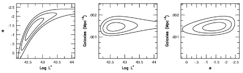
treated each curve as a probability distribution (i.e., with a unity normalization), and computed the likelihood that the observed sample of Ly fluxes is drawn from the resultant distribution. The results for the three parameters of this fit, , , and , the integral of the Schechter function down to our limiting flux (in units of galaxies Mpc-3), are shown in Figure 11; Table 5 lists the best-fitting parameters, along with their marginalized most-likely values and uncertainties. For completeness, Table 5 also gives the value of which is inferred from our most likely solution. As expected, the plots illustrate the familiar degeneracy between and : our best-fit solution has , but if is forced to brighter luminosities, decreases. The contours also demonstrate an asymmetry in the solutions, whereby extremely bright values of are included within the contours of probability, but faint values of the same quantity are not.
But perhaps the most interesting feature of the analysis concerns the effective volume of our survey. As in Section 2.1, the amount of space sampled by the observations depends critically on each galaxy’s Ly luminosity and equivalent width. Bright line-emitters with large equivalent widths can be identified well onto the wings of the filter, hence the survey volume associated with these objects is relatively large. Conversely, weak line-emitters, and objects with small equivalent widths can only be detected if they lie at the peak of the filter transmission curve. Thus, the survey volume for these objects is quite small. The effective volume for our observations is therefore a weighted average, which depends on the intrinsic properties of entire LAE sample.
This average can be computed from the data displayed in Figure 11. According to the figure, the space density of galaxies with emission-line brighter than ergs cm-2 s-1 (i.e., ergs s-1) is extremely well-defined, galaxies Mpc-3. Since this measurement comes from the detection of 160 galaxies brighter than the completeness limit, the data imply an effective survey volume of Mpc3. This is not the volume one would infer from the interference filter’s full-width at half-maximum: it is 25% smaller, or roughly the full-width of the filter at two-thirds maximum.
This difference is illustrated in Figure 10. The points show the space density of Ly galaxies one would derive simply by using the filter’s FWHM to define the survey volume; the solid line gives the Schechter (1976) function which best fits the data. The offset between the solid line and the dashed line, which represents the function after the application of the two convolution kernels, confirms the need for careful analysis when working with narrow-band data taken through a non-square bandpass.
The results of our maximum-likelihood calculation also suggest a simple definition for the effective transmission for our filter. As described in Section 2.1, a “characteristic” transmission is needed to convert the (bandpass-dependent) AB magnitude of an individual galaxy to monochromatic Ly flux. Rather than use the maximum transmission (which would underestimate the flux of all galaxies not at the filter peak), or adopt some complicated scheme which involves iterating on the luminosity function, one can simply choose the filter’s mean transmission within some limited wavelength range. Based on the results above, the filter’s full-width at two-thirds maximum seems an appropriate limit. This transmission, which is indicated by the arrow in Figure 4, is the value used to derive the fluxes and equivalent widths of Tables 2 and 3. If were to use to filter’s peak transmission instead of this characteristic value, the tabulated emission-line fluxes and equivalent widths would all be smaller.
The error bars quoted above for the space density of Ly emitters represent only the statistical uncertainty of the fits. They do not include the possible effects of large-scale structure within our survey volume. Specifically, if the linear bias factor for LAEs is two (see Gawiser et al., 2007, for an analysis of the objects’ clustering) then the expected fluctuation in the density of Ly emitters measured within a Mpc3 volume of space is . This value should be combined in quadrature with our formal statistical uncertainty.
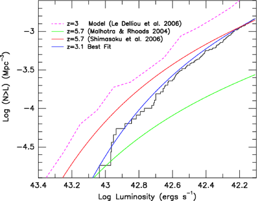
Since Ly galaxies have been observed at a number of redshifts, it is tempting to use our data to examine the evolution of the LAE luminosity function. Unfortunately, the samples obtained to date are not yet robust enough for this purpose. An example of the problem is shown in Figure 12, which compares our cumulative luminosity function (and our Schechter fit for ) to two measures of Ly galaxies at . As the figure illustrates, there are large differences between the measurements. If the Malhotra & Rhoads (2004) luminosity function is correct, then LAEs at are a factor of brighter and/or more numerous than their counterparts. However, if the LAE luminosity function of Shimasaku et al. (2006) is correct, then evolution is occurring in the opposite direction, i.e., the star-formation rate density is declining with time. Without better data, it is difficult to derive any conclusions about the evolution of these objects.
Figure 12 also plots our data against the predictions of a hierarchical model of galaxy formation (Le Delliou et al., 2005, 2006). As this comparison demonstrates, our luminosity function for LAEs lies slightly below that generated by theory. This is not surprising: one of the key parameters of the model, the escape fraction of Ly photons, was set using previous estimates of the density of LAEs. Unfortunately, these measurements were based on extremely small samples of objects, specifically, nine emitters from Kudritzki et al. (2000) and ten LAEs from Cowie & Hu (1998). Since these surveys inferred a larger space density of Ly emitters than measured in this paper, a mismatch between our data and the Le Delliou et al. (2006) models is neither unexpected nor significant.
6 Star Formation Rate Density at
Perhaps the most interesting result of our survey comes from a comparison of the galaxies’ Ly emission with their -band magnitudes. Both quantities measure star formation rate: Ly via the combination of Case B recombination theory and the H vs. star formation relation
| (5) |
(Kennicutt, 1998; Hu, Cowie, & McMahon, 1998), and , via population synthesis models of the rest-frame UV ()
| (6) |
(Kennicutt, 1998). If both of these calibrations hold for our sample of Ly emitters, then a plot of the two SFR indicators should scatter about a one-to-one relation.
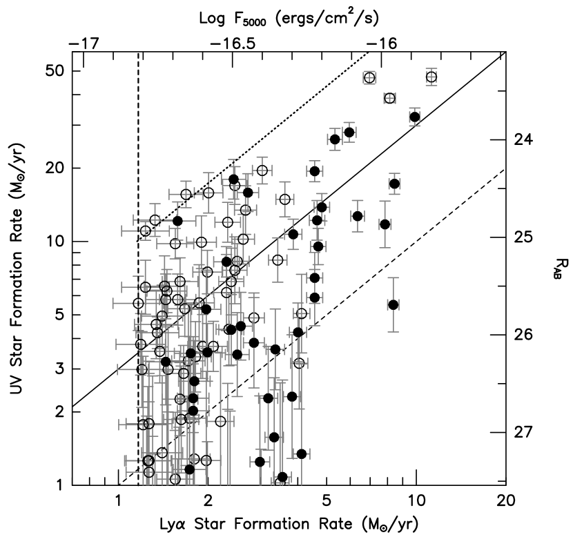
Figure 13 displays this plot. In the figure, galaxies with Ly star-formation rates less than yr-1 are excluded by our ergs cm-2 s-1 monochromatic flux limit, while objects with large UV star-formation rates, but weak Ly are eliminated by our equivalent width criterion. The latter is not a hard limit, since LAE colors range from , and it is the continuum that is used to define equivalent width. Nevertheless, if we adopt 1.4 as the upper limit on the median color of an Ly emitting galaxy (i.e., above the median color of the population), we obtain the dotted line shown in the figure.
Despite these selection effects, the Ly and UV continuum star-formation rates do seem to be correlated. However, there is an offset: the rates inferred from the UV are, on average, about three times higher than those derived from Ly. While the Ly SFR measurements are generally less than yr-1, the rest-frame UV values extend up to yr-1. This discrepancy has previously been seen in a sample of 20 LAEs at (Ajiki et al., 2003), and has two possible explanations.
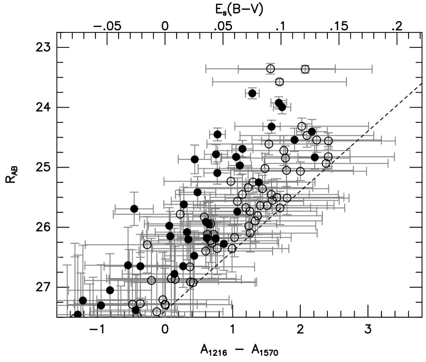
The most likely cause of the offset is the galaxies’ internal extinction. By studying local starburst galaxies, Calzetti (2001) has shown that a system’s ionized gas is typically attenuated more than its stars. In other words, while optical and IR emission-line ratios can usually be reproduced with a simple screen model, the shape of the UV continuum requires that the dust and stars be intermingled. For a self-consistent solution, Calzetti (2001) suggests
| (7) |
If we apply the Calzetti (2001) law to our sample of Ly emitters, then for the UV and Ly star-formation rates to be equal, the extinction within our LAEs must be as shown in Figure 14. According to the figure, in most cases it only requires a small amount of dust () to bring the two indicators into agreement. Figure 14 also suggests that internal extinction becomes more important in the brighter galaxies. This is consistent with observations of local starburst systems (e.g., Meurer et al., 1995), and is expected if the mass-metallicity relation seen in the local universe carries over to dust content.
Alternatively, the discrepancy between the Ly and UV continuum star-formation rates may simply be due to uncertainties in their estimators. Models which translate UV luminosity into star formation rate have almost a factor of two scatter and rely on a number of parameters, including the initial mass function and the timescale for star formation. The latter is particularly problematic. Ly photons are produced almost exclusively by extremely young ( Myr), massive () stars which ionize their surroundings. It therefore registers the instantaneous star-formation occurring in the galaxy. Conversely, continuum UV emission (at 1570 Å) can be produced by populations as old as Gyr; thus, it is a time-averaged quantity. If the star-formation rate in our Ly emitters has declined over time, then it is possible for UV measurements to systematically overestimate the present day star formation (Glazebrook et al., 1999).
If we assume that Ly emission is an accurate measure of star-formation, then it is possible to integrate the Schechter function to estimate the total contribution of LAEs to the star-formation rate density of the universe. We note that this procedure does carry some uncertainty. If we just consider galaxies brighter than our completeness limit ( ergs cm-2 s-1 or ergs s-1) then the star-formation rate density associated with LAEs is yr-1 Mpc-3, or yr-1 Mpc-3 if the internal extinction in these objects is . However, to compute the total star-formation rate density, we need to extrapolate the LAE luminosity function to fainter magnitudes, and even 160 objects is not sufficient to define to better than . Consequently, our data admit a range of solutions.
This is illustrated in Figure 15, which displays SFR likelihoods derived from the probabilities illustrated in Figure 11. As the figure shows, the most likely value for the LAE star-formation rate density of the universe (uncorrected for internal extinction) is yr-1 Mpc-3, while the median value of this quantity (defined as the point with equal amounts of probability above and below) is yr-1 Mpc-3. Moreover, these numbers are likely to be lower limits: if the discrepancy seen in Figure 13 is due to internal extinction, then the true SFR density is probably times higher.
The numbers above indicate that at , the star-formation rate density associated with Ly emitters is comparable to that found for Lyman-break galaxies. Before correcting for extinction, our number for the LAE star-formation rate density is yr-1 Mpc-3. For comparison, the LBG star-formation rate density at (before extinction) is yr-1 Mpc-3 (Madau et al., 1998; Steidel et al., 1999). It is true that internal extinction within Lyman-break galaxies is typically larger than it is in our LAEs, (Steidel et al., 1999). However, according to the Calzetti (2001) extinction law, the effect of dust on the emission line flux of a galaxy is much greater than that on the stellar continuum. Consequently, our dust corrected SFR density for LAEs, yr-1 Mpc-3, is of the LBG value. Of course, given the extrapolations and corrections required to make this comparison, this number is highly uncertain.
7 Discussion
The space density of Ly emitters shown in Figure 11 translates into a surface density of arcmin-2 per unit redshift interval above our completeness limit. This number is similar to that derived by Thommes & Meisenheimer (2005), under the assumption that the LAE phenomenon is associated with the creation of elliptical galaxies and spiral bulges. It is also consistent with the semi-analytical hierarchical structure calculations of Le Delliou et al. (2005), though the latter predict a slightly larger number of LAEs than found in this paper. This difference is not significant, since the Le Delliou et al. (2005) models have been adjusted to match the previous small-volume Ly surveys of Kudritzki et al. (2000) and Cowie & Hu (1998). A re-scaling of the escape fraction of Ly photons solves the discrepancy, and maintains the match between the predictions and the faint-end slope of the galaxy luminosity function.
More notable is the excellent agreement between the Le Delliou et al. (2006) simulations and the observed distribution of Ly equivalent widths (Figure 9). Both are very well-fit via an exponential with a large ( Å) scale length. Moreover, the models also predict that the scale length observed for a magnitude-limited sample of galaxies (such as that produced by the Lyman-break technique) will be much smaller than that found via an emission-line survey. This is consistent with the LBG results found by Shapley et al. (2003).
Nevertheless, we should emphasize that the LAEs detected in this survey are probably not primordial galaxies in their initial stages of star-formation. Very few of the objects have the extremely high equivalent widths calculated for stellar populations with top-heavy initial mass functions. More importantly, the scatter in the galaxies’ colors, along with the offset between the Ly and UV continuum star-formation rates, suggests that these objects possess a non-negligible amount of dust. The existence of this dust argues against the Pop III interpretation of Ly emitters (Jimenez & Haiman, 2006).
The extremely strong line emission associated with LAEs makes these objects especially suitable for probing the evolution of galaxies and structure in the distant universe. The space density of emitters shown in Figure 11 translates into a surface density of arcmin-2 per unit redshift interval above our completeness limit. This, coupled with our measured luminosity function, implies that in the absence of evolution, there are LAEs arcmin-2 brighter than ergs cm-2 s-1 in the redshift range . Wide field integral field units, such as those being designed for ESO (Henault et al., 2004) and the Hobby-Eberly Telescope (Hill et al., 2006) will therefore be able to find large numbers of Ly emitters in a single pointing. Moreover, because the faint-end of the luminosity function is steep (), the density of LAEs goes linearly with survey depth. Dropping the flux limit by a factor of two (to ergs cm-2 s-1) will roughly double the number of LAEs in the sample.
With an integral-field spectrograph, it is also possible to increase the sample of high-redshift galaxies by identifying objects with equivalent widths lower than our detection threshold of 80 Å ( Å in the LAE rest frame). However, the gain in doing so is likely to be small: according to Figure 9, Ly rest-frame equivalent widths e-fold with a scale length of Å. If this law extrapolates to weaker-lined systems, as suggested by the models of Le Delliou et al. (2006), then most Ly emitters are already being detected, and pushing the observations to lower equivalent widths will only increase the number counts by . Furthermore, as the data of Hogg et al. (1998) demonstrate, contamination by foreground [O II] objects increases rapidly once the equivalent width cutoff drops below Å in the observers frame (or Å in the rest frame of Ly). Unless one can accept a large increase in the fraction of contaminants, surveys for high-redshift galaxies need to either stay above this threshold, or extend to the near-IR (to detect H and [O III] in the interlopers).
References
- Ajiki et al. (2003) Ajiki, M., Taniguchi, Y., Fujita, S.S., Shioya, Y., Nagao, T., Murayama, T., Yamada, S., Umeda, K., & Komiyama, Y. 2003, AJ, 126, 2091
- Alexander et al. (2003) Alexander, D.M., Bauer, F.E., Brandt, W.N., Schneider, D.P., Hornschemeier, A.E., Vignali, C., Barger, A.J., Broos, P.S., Cowie, L.L., Garmire, G.P., Townsley, L.K., Bautz, M.W., Chartas, G., & Sargent, W.L.W. 2003, AJ, 126, 539
- Blake & Glazebrook (2003) Blake, C., & Glazebrook, K. 2003, ApJ, 594, 665
- Bruzual & Charlot (2003) Bruzual, G., & Charlot, S. 2003, MNRAS, 344, 1000
- Calzetti (2001) Calzetti, D. 2001, PASP, 113, 1449
- Charlot & Fall (1993) Charlot, S., & Fall, S.M. 1993, ApJ, 415, 580
- Ciardullo et al. (2002) Ciardullo, R., Feldmeier, J.J., Krelove, K., Bartlett, R., Jacoby, G.H., & Gronwall, C. 2002, ApJ, 566, 784
- Ciardullo et al. (1989) Ciardullo, R., Jacoby, G.H., Ford, H.C., & Neill, J.D. 1989, ApJ, 339, 53
- Cowie & Hu (1998) Cowie, L.L., & Hu, E.M. 1998, AJ, 115, 1319
- Dawson et al. (2004) Dawson, S., Rhoads, J.E., Malhotra, S., Stern, D., Dey, A., Spinrad, H., Jannuzi, B.T., Wang, J.X., & Landes, E. 2004, ApJ, 617, 707
- Jimenez & Haiman (2006) Jimenez, R., & Haiman, Z. 2006, Nature, 440, 501
- De Propis et al. (1993) De Propris, R., Pritchet, C.J., Hartwick, F.D.A., & Hickson, P. 1993, AJ, 105, 1243
- Eather & Reasoner (1969) Eather, R.H., & Reasoner, D.L. 1969, Appl. Optics, 8, 227
- Eddington (1913) Eddington, A.S. 1913, MNRAS, 73, 359
- Eddington (1940) Eddington, A.S. 1940, MNRAS, 100, 354
- Feldmeier et al. (2003) Feldmeier, J.J., Ciardullo, R., Jacoby, G.H., & Durrell, P.R. 2003, ApJS, 145, 65
- Fujita et al. (2003) Fujita, S.S., Ajiki, M., Shioya, Y., Nagao, T., Murayama, T., Taniguchi, Y., Okamura, S., Ouchi, M., Shimasaku, K., Doi, M., Furusawa, H., Hamabe, M., Kimura, M., Komiyama, Y., Miyazaki, M., Miyazaki, S., Nakata, F., Sekiguchi, M., Yagi, M., Yasuda, N., Matsuda, Y., Tamura, H., Hayashino, T., Kodaira, K., Karoji, H., Yamada, T., Ohta, K., & Umemura, M. 2003, AJ, 125, 13
- Gallego et al. (2002) Gallego, J., García-Dabó, C.E., Zamorano, J., Aragón-Salamanca, A., & Rego, M. 2002, ApJ, 570, L1
- Gawiser et al. (2006a) Gawiser, E., van Dokkum, P.G., Gronwall, C., Ciardullo, R., Blanc, G., Castander, F.J., Feldmeier, J., Francke, H., Franx, M., Haberzettl, L., Herrera, D., Hickey, T., Infante, L., Lira, P., Maza, J., Quadri, R., Richardson, A., Schawinski, K., Schirmer, M., Taylor, E.N., Treister, E., Urry, C.M., & Virani, S.N. 2006a, ApJ, 642, L13
- Gawiser et al. (2006b) Gawiser, E., et al. 2006b, ApJS, 162, 1
- Gawiser et al. (2007) Gawiser, E., et al. 2007, in preparation
- Giacconi et al. (2002) Giacconi, R., Zirm, A., Wang, J.X., Rosati, P., Nonino, M., Tozzi, P., Gilli, R., Mainieri, V., Hasinger, G., Kewley, L., Bergeron, J., Borgani, S., Gilmozzi, R., Grogin, N., Koekemoer, A., Schreier, E., Zheng, W., & Norman, C. 2002, ApJS, 139, 369
- Giavalisco (2002) Giavalisco, M. 2002, ARA&A, 40, 579
- Giavalisco et al. (2004) Giavalisco, M., et al. 2004, ApJ, 600, L93
- Glazebrook et al. (1999) Glazebrook, K., Blake, C., Economou, F., Lilly, S., & Colless, M. 1999, MNRAS, 306, 843
- Hanes & Whittaker (1987) Hanes, D.A., & Whittaker, D.G. 1987, AJ, 94, 906
- Hayashino et al. (2004) Hayashino, T., Matsuda, Y., Tamura, H., Yamauchi, R., Yamada, T., Ajiki, M., Fujita, S.S., Murayama, T., Nagao, T., Ohta, K., Okamura, S., Ouchi, M., Shimasaku, K., Shioya, Y., & Taniguchi, Y. 2004, AJ, 128, 2073
- Henault et al. (2004) Henault, F., Bacon, R., Content, R., Lantz, B., Laurent, F., Lemonnier, J.-P., & Morris, S.L. 2004, in Proc. SPIE Vol. 5249, Optical Design and Engineering, ed. L. Mazuray, P.J. Rogers, & R. Wartmann (Bellingham: SPIE), 134
- Hill et al. (2006) Hill, G.J., MacQueen, P.J., Palunas, P., Kelz, A., Roth, M.M., Gebhardt, K., & Grupp, F. 2006, New Astronomy Review, 50, 378
- Hogg et al. (1998) Hogg, D.W., Cohen, J.G., Blandford, R., & Pahre, M.A. 1998, ApJ, 504, 622
- Hu, Cowie, & McMahon (1998) Hu, E.M., Cowie, L.L., & McMahon, R.G. 1998, ApJ, 502, L99
- Jacoby et al. (1989) Jacoby, G.H., Ciardullo, R., Booth, J., & Ford, H.C. 1989, ApJ, 344, 704
- Jacoby et al. (1987) Jacoby, G.H., Quigley, R.J., & Africano, J.L. 1987, PASP, 99, 672
- Kennicutt (1998) Kennicutt, R.C. 1998, ARA&A, 36, 189
- Kodaira et al. (2003) Kodaira, K., et al. 2003, PASJ, 55, L17
- Koehler et al. (2007) Koehler, R.S., Schuecker, P., & Gebhardt, K. 2007, A&A, 462, 7
- Kudritzki et al. (2000) Kudritzki, R.-P., Méndez, R.H., Feldmeier, J.J., Ciardullo, R., Jacoby, G.H., Freeman, K.C., Arnaboldi, M., Capaccioli, M., Gerhard, O., & Ford, H.C. 2000, ApJ, 536, 19
- Le Delliou et al. (2005) Le Delliou, M., Lacey, C., Baugh, C.M., Guiderdoni, B., Bacon, R., Courtois, H., Sousbie, T., & Morris, S.L. 2005, MNRAS, 357, L11
- Le Delliou et al. (2006) Le Delliou, M., Lacey, C.G., Baugh, C.M., & Morris, S.L. 2006, MNRAS, 365, 712
- Lehmer et al. (2005) Lehmer, B.D., Brandt, W.N., Alexander, D.M., Bauer, F.E., Schneider, D.P., Tozzi, P., Bergeron, J., Garmire, G.P., Giacconi, R., Gilli, R., Hasinger, G., Hornschemeier, A.E., Koekemoer, A.M., Mainieri, V., Miyaji, T., Nonino, M., Rosati, P., Silverman, J.D., Szokoly, G., & Vignali, C. 2005, ApJS, 161, 21
- Lehmer et al. (2007) Lehmer, B.D., Brandt, W.N., Alexander, D.M., Bell, E.F., McIntosh, D.H., Bauer, F.E., Hasinger, G., Mainieri, V., Miyaji, T., Schneider, D.P., & Steffen, A.T. ApJ, 657, 681
- Lira et al. (2007) Lira, P., et al. 2007, in preparation
- Madau et al. (1996) Madau, P., Ferguson, H.C., Dickinson, M.E., Giavalisco, M., Steidel, C.C., & Fruchter, A. 1996, MNRAS, 283, 1388
- Madau et al. (1998) Madau, P., Pozzetti, L., & Dickinson, M. 1998, ApJ, 498, 106
- Malhotra & Rhoads (2002) Malhotra, S., & Rhoads, J.E. 2002, ApJ, 565, L71
- Malhotra & Rhoads (2004) Malhotra, S., & Rhoads, J.E. 2004, ApJ, 617, L5
- Meier & Terlevich (1981) Meier, D.L., & Terlevich, R. 1981, ApJ, 246, L109
- Meurer et al. (1995) Meurer, G.R., Heckman, T.M., Leitherer, C., Kinney, A., Robert, C., & Garnett, D.R. 1995, AJ, 110, 2665
- Monet et al. (1998) Monet, D., Bird, A., Canzian, B., Dahn, C., Guetter, H., Harris, H., Henden, A., Levine, S., Luginbuhl, C., Monet, A.K.B., Rhodes, A., Riepe, B., Sell, S., Stone, R., Vrba, F., & Walker, R. 1998, PMM USNO-A2.0: A Catalogue of Astrometric Standards (Washington, DC: US Naval Obs.)
- Ouchi et al. (2003) Ouchi, M., Shimasaku, K., Furusawa, H., Miyazaki, M., Doi, M., Hamabe, M., Hayashino, T., Kimura, M., Kodaira, K., Komiyama, Y., Matsuda, Y., Miyazaki, S., Nakata, F., Okamura, S., Sekiguchi, M., Shioya, Y., Tamura, H., Taniguchi, Y., Yagi, M., & Yasuda, N. 2003, ApJ, 582, 60
- Ranalli et al. (2003) Ranalli, P., Comastri, A., & Setti, G. 2003, A&A, 399, 39
- Rhoads et al. (2003) Rhoads, J.E., Dey, A., Malhotra, S., Stern, D., Spinrad, H., Jannuzi, B.T., Dawson, S., Brown, M., & Landes, E. 2003, AJ, 125, 1006
- Rhoads et al. (2000) Rhoads, J.E., Malhotra, S., Dey, A., Stern, D., Spinrad, H., & Jannuzi, B.T. 2000, ApJ, 545, L85
- Rix et al. (2004) Rix, H.-W., Barden, M., Beckwith, S.V.W., Bell, E.F., Borch, A., Caldwell, J.A.R., Häussler, B., Jahnke, K., Jogee, S., McIntosh, D.H., Meisenheimer, K., Peng, C.Y., Sanchez, S.F., Somerville, R.S., Wisotzki, L., & Wolf, C. 2004, ApJS, 152, 163
- Schechter (1976) Schechter, P. 1976, ApJ, 203, 297
- Seo & Eisenstein (2003) Seo, H.-J., & Eisenstein, D.J. 2003, ApJ, 598, 720
- Shapley et al. (2003) Shapley, A.E., Steidel, C.C., Pettini, M., & Adelberger, K.L. 2003, ApJ, 588, 65
- Shimasaku et al. (2004) Shimasaku, K., Hayashino, T., Matsuda, Y., Ouchi, M., Ohta, K., Okamura, S., Tamura, H., Yamada, T., & Yamauchi, R. 2004, ApJ, 605, L93
- Shimasaku et al. (2006) Shimasaku, K., Kashikawa, N., Doi, M., Ly, C., Malkan, M.A., Matsuda, Y., Ouchi, M., Hayashino, T., Iye, M., Motohara, K., Murayama, T., Nagao, T., Ohta, K., Okamura, S., Sasaki, T., Shioya, Y., & Taniguchi, Y. 2006, PASJ, 58, 313
- Steidel et al. (1999) Steidel, C.C., Adelberger, K.L., Giavalisco, M., Dickinson, M., & Pettini, M. 1999, ApJ, 519, 1
- Steidel et al. (2000) Steidel, C.C., Adelberger, K.L., Shapley, A.E., Pettini, M., Dickinson, M., & Giavalisco, M. 2000, ApJ, 532, 170
- Steidel et al. (2003) Steidel, C.C., Adelberger, K.L., Shapley, A.E., Pettini, M., Dickinson, M., & Giavalisco, M. 2003, ApJ, 592, 728
- Steidel et al. (1996a) Steidel C.C., Giavalisco, M., Dickinson, M., & Adelberger, K.L. 1996a, AJ, 112, 352
- Steidel et al. (1996b) Steidel, C.C., Giavalisco, M., Pettini, M., Dickinson, M., & Adelberger, K.L. 1996b, ApJ, 462, L17
- Stiavelli et al. (2001) Stiavelli, M., Scarlata, C., Panagia, N., Treu, T., Bertin, G., & Bertola, F. 2001, ApJ, 561, L37
- Stone (1977) Stone, R.P.S. 1977, ApJ, 218, 767
- Taniguchi et al. (2005) Taniguchi, Y., et al. 2005, PASJ, 57, 165
- Tapken et al. (2006) Tapken, C., Appenzeller, I., Gabasch, A., Heidt, J., Hopp, U., Bender, R., Mehlert, D., Noll, S., Seitz, S., & Seifert, W. 2006, A&A, 455, 145
- Teplitz et al. (2003) Teplitz, H.I., Collins, N.R., Gardner, J.P., Hill, R.S., & Rhodes, J. 2003, ApJ, 589, 704
- Thommes & Meisenheimer (2005) Thommes, E., & Meisenheimer, K. 2005, A&A, 430, 877
- Thompson, Djorgovski, & Trauger (1995) Thompson, D., Djorgovski, S., & Trauger, J. 1995, AJ, 110, 963
- Venemans et al. (2005) Venemans, B.P., Röttgering, H.J.A., Miley, G.K., Kurk, J.D., de Breuck, C., Overzier, R.A., van Breugel, W.J.M., Carilli, C.L., Ford, H., Heckman, T., Pentericci, L., & McCarthy, P. 2005, A&A, 431, 793
- Virani et al. (2006) Virani, S.N., Treister, E., Urry, C.M., & Gawiser, E. 2006, AJ, 131, 2373
| Exposure | Seeing | Active | |
|---|---|---|---|
| UT Date | (hr) | () | CCDs |
| 6 Oct 2002 | 2.0 | 8 | |
| 12 Oct 2002 | 1.7 | 8 | |
| 4 Jan 2003 | 2.0 | 8 | |
| 5 Jan 2003 | 3.0 | 8 | |
| 6 Jan 2003 | 3.0 | 8 | |
| 29 Nov 2003 | 2.5 | 7 | |
| 1 Dec 2003 | 1.7 | 7 | |
| 23 Jan 2004 | 2.3 | 7 | |
| 24 Jan 2004 | 2.0 | 7 | |
| 25 Jan 2004 | 2.5 | 7 | |
| 16 Feb 2004 | 1.1 | 7 | |
| 17 Feb 2004 | 0.8 | 7 | |
| 18 Feb 2004 | 1.3 | 7 | |
| 19 Feb 2004 | 1.2 | 7 | |
| 20 Feb 2004 | 0.9 | 7 |
| ID | (2000) | (2000) | Log | Equivalent Width |
|---|---|---|---|---|
| 1aaCandidate AGN | 03:33:16.86 | 28:01:05.2 | 449 | |
| 2 | 03:33:12.72 | 27:42:47.1 | 392 | |
| 3bbForeground AGN | 03:33:07.61 | 27:51:27.0 | 92 | |
| 4 | 03:32:18.79 | 27:42:48.3 | 251 | |
| 5 | 03:32:47.51 | 27:58:07.6 | 235 | |
| 6 | 03:32:52.68 | 27:48:09.4 | 272 | |
| 7 | 03:31:44.99 | 27:35:32.9 | 248 | |
| 8 | 03:31:54.89 | 27:51:21.0 | 310 | |
| 9 | 03:31:40.16 | 28:03:07.5 | 116 | |
| 10 | 03:33:22.45 | 27:46:36.9 | 143 |
| ID | (2000) | (2000) | Log | Equivalent Width |
|---|---|---|---|---|
| 163 | 03:33:14.82 | 27:44:09.1 | 380 | |
| 164 | 03:32:08.46 | 27:48:43.5 | 445 | |
| 165 | 03:33:26.22 | 27:46:09.0 | 468 | |
| 166 | 03:33:11.73 | 27:46:51.7 | 312 | |
| 167 | 03:31:26.49 | 27:50:34.3 | 209 | |
| 168 | 03:33:05.64 | 27:52:47.2 | 284 | |
| 169 | 03:31:50.46 | 27:41:15.2 | 364 | |
| 170 | 03:33:17.68 | 27:45:44.5 | 109 | |
| 171 | 03:31:48.98 | 27:53:38.7 | 322 | |
| 172 | 03:33:10.77 | 27:52:41.4 | 356 |
| Log | (mag) | Log | (mag) |
|---|---|---|---|
| 0.022 | 0.065 | ||
| 0.024 | 0.073 | ||
| 0.026 | 0.082 | ||
| 0.031 | 0.104 | ||
| 0.033 | 0.125 | ||
| 0.038 | 0.158 | ||
| 0.042 | 0.204 | ||
| 0.050 | 0.264 | ||
| 0.058 | 0.329 |
| Parameter | Best Solution | Marginalized Values |
|---|---|---|
| Log (ergs s-1) | 42.66 | |
| ergs s-1) Mpc-3 | ||
| (Mpc-3) | … |