Monte Carlo simulations of ${\rm Rb_{2}MnF_{4}}$, a classical Heisenberg antiferromagnet in two-dimensions with dipolar interaction

Abstract

We study the phase diagram of a quasi-two dimensional magnetic system ${\rm Rb_{2}MnF_{4}}$ with Monte Carlo simulations of a classical Heisenberg spin Hamiltonian which includes the dipolar interactions between ${\rm Mn}^{2+}$ spins. Our simulations reveal an Ising-like antiferromagnetic phase at low magnetic fields and an XY phase at high magnetic fields. The boundary between Ising and XY phases is analyzed with a recently proposed finite size scaling technique and found to be consistent with a bicritical point at $T=0$. We discuss the computational techniques used to handle the weak dipolar interaction and the difference between our phase diagram and the experimental results.

I Introduction

The phase diagram of anisotropic Heisenberg antiferromagnets has been studied with renormalization group (RG) methodsKosterlitz et al. (1976); Nelson and Rudnick (1975); Pelcovits and Nelson (1976); Nelson (1976); Nelson and Pelcovits (1977) and Monte Carlo simulations.Landau and Binder (1978, 1981); Holtschneider et al. (2005); Zhou et al. (2006) In three dimensions, RG calculations for $4-\epsilon$ dimensions and Monte Carlo simulations have found an Ising-like antiferromagnetic (AF) phase at low magnetic fields and an XY phase at high fields, separated by a 1st order spin-flop transition line. The spin-flop transition line terminates at a bicritical point (BCP), where it meets the phase boundary between the XY phase and the paramagnetic (PM) phase, and the AF-PM phase boundary. In two-dimensions, due to the Mermin-Wagner theorem,Mermin and Wagner (1966) a BCP with $O(3)$ symmetry has to be at zero-temperature, which was confirmed by RG calculations in $2+\epsilon$ dimensions for the anisotropic non-linear $\sigma$-model.Pelcovits and Nelson (1976); Nelson and Pelcovits (1977) The XY-PM phase boundary and AF-PM phase boundary are exponentially close to each other while the PM phase sandwiched in between narrows as $\exp(-4\pi/T)$. On the other hand, the continuum field theory of this model contains an infinite number of relevant perturbations beyond the anisotropic nonlinear $\sigma$-model. Thus, it is also valid to argue that the multicritical point may not be $O(3)$ symmetric and occurs at a finite temperature.Pelissetto and Vicari (2007) One would look for numerical evidence that distinguishes different scenarios. However, Monte Carlo simulations have been unable to trace the phase boundaries of the XY and AF phases to sufficiently low temperatures, due to the exponentially large correlation length. Recently, a novel finite size scaling analysis was used to interpret the data from Monte Carlo simulations.Zhou et al. (2006) It was found that the apparent spin-flop transition line was actually consistent with a zero temperature BCP. An additional continuous degeneracy in the ground state at the spin-flop field has also been recently discovered.Holtschneider et al. (2007) The ground state actually bears some similarities to a tetracritical phase; thus it was argued that the “hidden bicritical point” might be relabeled as the “hidden tetracritical point.”

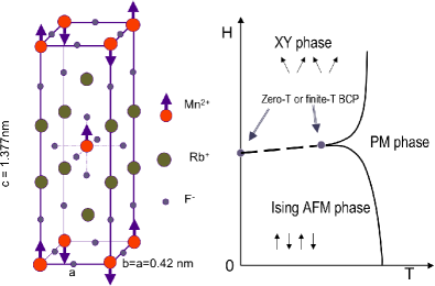
Figure 1: (color online) The unit cell of ${\rm Rb_{2}MnF_{4}}$ and the schematic phase diagram. If the BCP is at $T=0$, the dashed line actually represents two very close second order phase boundaries. If the BCP is at a finite temperature, the dashed line represents a single first order phase transition. The theoretical XY phase is found to have transverse AF order in neutron scattering experiments.

In real materials, an ideal two-dimensional Heisenberg spin system has not been found, since in a three-dimensional system, the interactions between spins can never be completely restricted to two dimensions. Nevertheless, ${\rm Rb_{2}MnF_{4}}$ is a very good quasi-two-dimensional Heisenberg antiferromagnet. In this layered compound, ${\rm Mn}^{2+}$ ions with spin-5/2 reside on (001) planes, as shown in Fig. 1. Adjacent planes are widely separated by ${\rm Rb}^{+}$ ions, so that the exchange interactions between magnetic ions in different planes are negligible. The antiferromagnetic order parameter has been accurately measured with neutron scattering experiments,Birgeneau et al. (1970) and analyzed with spin-wave theory.de Wijin et al. (1973) The theoretical model with only nearest neighbor exchanges and a staggered magnetic field accounts for the experimental data very well. In the right hand portion of Fig. 1 we show a schematic phase diagram that summarizes the prevailing theoretical alternatives and experimental data for ${\rm Rb_{2}MnF_{4}}$. On the other hand, the large magnetic moment of ${\rm Mn}^{2+}$ ions makes it possible to model the spins with classical vectors. Therefore, it is an excellent system to test theoretical predictions for two-dimensional Heisenberg spin systems, given that the effective anisotropy due to the dipolar interaction is accounted for.Christianson et al. (2001) Obviously, the dipolar interaction plays an important role in this system, as it provides the effective anisotropy that stabilizes the low-field AF phase and could mediate a dimensional crossover from two dimensions to three dimensions in the real material. With the in-plane isotropic exchange interaction and the dipolar interaction, the Neel temperature at zero-field was calculated by Monte Carlo simulations to be 39.7$\pm$0.1 K,Lee et al. (2003) slightly higher than the experimental value 38.5$\pm$1.0 K.de Wijin et al. (1973); Breed (1967) Following the previous research,Lee et al. (2003) we performed extensive Monte Carlo simulations in both zero and non-zero magnetic fields to construct the full phase diagram and compare it with the experiments.Cowley et al. (1993) We hope to see our model reproduce the “apparent” BCP at approximately $T=30$K, as seen in the experiments. To determine the phase diagram in the thermodynamic limit, we used different finite size scaling analyses for different phase boundaries. In particular, the “apparent” spin flop transition has to be examined with the novel finite size scaling method developed in Ref. Zhou et al., 2006, and it is actually found to be consistent with a zero temperature BCP.

The Hamiltonian of our model reads

$${\cal H}= - JS(S+1)\sum_{<i,j>}{\bf S}_{i}\cdot{\bf S}_{j}-{US^{2}\over 2}\sum_{i\neq j,\;\alpha,\beta}S_{i}^{\alpha}{\cal D}_{ij}^{\alpha\beta}S_{j}^{\beta}$$ (1)

$$- \sum_{i}Sg\mu_{B}{\bf h}\cdot{\bf S}_{i},$$

where $S=5/2$, ${\bf S}_{i}$ are three dimensional unit vectors, $J=0.6544$meV, the dipolar interaction constantAshcroft and Mermin (1976) $U=0.214727$meVų, the Landé $g$-factor $g=2$, the external magnetic field ${{\bf h}}$ is fixed in the $z$-direction, and the summation over $\left<i,j\right>$ is over all nearest neighbor pairs. The dipolar interaction tensor ${\cal D}$ is given by:

$${\cal D}_{ij}^{\alpha\beta}=(3r_{ij}^{\alpha}r_{ij}^{\beta}-r^{2}_{ij}\delta_{\alpha\beta})r_{ij}^{-5}.$$ (2)

The ${\rm Mn}^{2+}$ ions are located on a body centered tetragonal lattice, with in-plane lattice constant $a=4.2$Å, and $c$-axis lattice constant $c=13.77$Å. However, it is known that the dipolar interaction between two tetragonal sublattices nearly vanishes due to the geometric arrangement of the moments.Lines (1967); Birgeneau et al. (1970) Therefore, besides a few simulations with two sublattices performed to check the validity of this assumption, we included only one sublattice in most of our simulations, which allowed us to simplify the dipolar summation and to run simulations for larger systems. Because the inter-layer interaction is weak, we have included up to four layers of spins in our simulations, with open boundary condition in the $z$ direction. Each layer is a square lattice with lattice constant equal to $a$ and the distance between adjacent layers equal to $c$.

The Hamiltonian Eq. (1) is an approximation of the actual quantum mechanical Hamiltonian, where spin operators have been replaced with classical vector spins $S{\bf S}_{i}$ or $\sqrt{S(S+1)}{\bf S}_{i}$. Here some ambiguities arise as to whether $S$ or $\sqrt{S(S+1)}$ should be used. For the dipolar term, we assume that the magnetic field generated by a spin is a dipole field of a magnetic moment $gS\mu_{B}$, and the dipolar interaction energy of a second spin with moment $gS\mu_{B}$ in this field is clearly proportional to $S^{2}$. This approximation guarantees that the total dipolar energy of a ferromagnetic configuration agrees with macroscopic classical magnetostatics of bulk materials. The exchange term is more ambiguous. One can argue that $S(S+1)$ follows from the quantum mechanical origin of the exchange interaction. After all, the appropriate constant should reproduce the correct spin wave spectrum or the critical temperature within acceptable error bars. There is no guarantee that both of them can be accurately reproduced with the same classical approximation. In general, by adopting the classical approximation to spins, one admits an error possibly of order $1/S$ in some quantities. To justify our choice in Eq. (1), we first found that the critical temperature at zero field of Eq. (1) was quite close to the experimental value, then we turned on the magnetic fields to explore the full phase diagram. It is unlikely that the entire experimental phase diagram would be reproduced exactly including the spin-flop field. However, our Monte Carlo simulations should exhibit the same critical behavior as the real material, given that they are in the same universality class. In particular, we want to test if there is a “real” BCP at a finite temperature due to the long-range nature of the dipolar interaction.

This paper is organized as the following: In Sec. II, we briefly review the simulation techniques used in this research, especially those designed to handle long-range, but very weak, dipolar interaction; in Sec. III, we present the results from simulations performed near each phase boundary; in Sec. IV we discuss the results and give our conclusions.

II Monte Carlo methods

II.1 Dipole summation

Direct evaluation of the dipolar energy in Eq. (1) should be avoided because the computational cost of direct evaluation scales as $O(N^{2})$ where $N$ is the number of spins, and the periodic boundary condition needs to be satisfied. In our simulations we have as many as $8\times 10^{4}$ spins and need to evaluate the dipolar energy repeatedly. Therefore, a fast algorithm for dipolar interaction is required. We used the Benson and Mills algorithmBenson and Mills (1969) which employs the fast Fourier transformation of the spins to reduce the computational cost to $O(N\ln N)$. After Fourier transform, the dipolar sum in Eq. (1) can be written as

$$\sum_{n,n^{\prime},\alpha,\beta,{\bf q}}D_{nn^{\prime}}^{\alpha\beta}({\bf q})S^{\alpha}_{n}({\bf q})S^{\beta}_{n^{\prime}}(-{\bf q}),$$ (3)

where $n$ and $n^{\prime}$ label the different layers of the system, ${\bf q}$ is the in-plane wave vector, and $D_{nn^{\prime}}^{\alpha\beta}({\bf q})$ is the Fourier transform of ${\cal D}_{ij}^{\alpha\beta}$. This expression is less costly to evaluate than the Eq. (2), since the double summation over all the spins is replaced by a single summation over the wave vectors, and $D_{nn^{\prime}}^{\alpha\beta}({\bf q})$ are constants which can be calculated quickly in the initialization stage of the simulation. Explicit expressions for $D_{nn^{\prime}}^{\alpha\beta}({\bf q})$ were first derived in Ref. Benson and Mills, 1969, and were reproduced in Ref. Costa Filho et al., 2000 with more detail and clarity.

II.2 Monte Carlo updating scheme and histogram reweighting

In Monte Carlo simulations of magnetic spin systems, cluster algorithms offer the benefit of reduced correlation times. In Ref. Lee et al., 2003, the Wolff cluster algorithmWolff (1989) was used to generate new spin configurations based on the isotropic exchange term in the Hamiltonian. Although the Wolff algorithm is rejection-free by itself, the new configuration then has to be accepted or rejected with a Metropolis algorithm according to its dipolar and Zeeman energy. The changes in the dipolar energy and Zeeman energy are roughly proportional to the size of the cluster generated by the Wolff algorithm. When these changes are larger than $k_{B}T$, the number of rejections rapidly increases, leading to substantially lower efficiency. This problem occurs when the magnetic field is typically several Tesla in our simulations. On the other hand, in the paramagnetic phase or one of the ordered phases, the cluster size is small, the change in dipolar energy is also small. It, thus, becomes redundant to evaluate the dipolar energy after every small change in the spin configuration.

Since there are no rejection free algorithms for the dipolar interaction, and the dipolar energy only contributes a fraction of about 0.1 per cent to the total energy in our simulations, one of our strategies to handle the dipolar interaction is to accumulate a series of single spin flips before evaluating the dipolar energy, then accept or reject this series of flips as a whole with the Metropolis algorithm depending on the change of the dipolar energy. The number of single spin flips for each Metropolis step can be adjusted in the simulation so that the average acceptance ratio is about 0.5, at which the Metropolis algorithm is most efficient. We used the rejection-free heat-bath algorithmMiyatake et al. (1986); Loison et al. (2004); Zhou et al. (2004) to perform single spin flips, which handles both the isotropic exchange and Zeeman terms in the Hamiltonian on the same footing.

Although fast Fourier transform significantly reduces the computational cost of dipolar interaction, this part is still the bottle-neck of the simulation. Therefore, we want to further reduce the number of dipolar energy evaluations. To this end, we separate a short-range dipolar interaction from the full dipolar interaction. The short-range part can be defined with an cutoff in distance. In our simulations, we have included the up to fifth nearest in-plane neighbor of each spin, and the spins directly above or below it in the adjacent layer of the same sublattice, to form the short range dipolar interaction. This short-range dipolar interaction can be handled with the heat-bath algorithm on the same footing with the exchange and the Zeeman term. The extra cost of evaluating local fields produced by the additional 22 neighboring spins is insignificant. With this modification in single spin updates, the Metropolis algorithm should be performed with respect to the change in the long-range dipolar interaction, i.e., the difference between the total dipolar energy and the short-range dipolar energy. Since this long range dipolar energy is typically a small fraction (about 1 per cent) of the total dipolar energy, it is justified to accumulate many single spin flips before refreshing the total dipolar energy.

We have found that the long-range dipolar energy in our simulations is usually a fraction of about 0.001 per cent of the total energy, which is actually comparable to $k_{B}T$. This allows us to further simplify the above algorithm by removing the Metropolis step in the simulation, while we simply calculate and record the full dipolar energy for each configuration whose energies and magnetizations are stored for histogram reweighting. In the end, we get a Markov chain of configurations from the simulation generated with a modified Hamiltonian

$${\cal H}^{\prime}={\cal H}_{\rm exchange}+{\cal H}_{\rm Zeeman}+{\cal H}_{\rm short},$$ (4)

where the the first two terms are the exchange and Zeeman terms in Eq. (1), and the last term is the short-range dipolar interaction. For those configurations selected for computing thermodynamic averages, we calculate and record ${\cal H}^{\prime}$, ${\cal H}_{\rm short}$, their full dipolar energy $H_{\rm dipole}$, staggered magnetization of each layer

$${\bf M}^{\dagger}_{l}={1\over L^{2}}\sum_{i,j}(-1)^{i+j}{\bf S}_{ijl},$$ (5)

where $L$ is the size of each layer and the index $l$ is the layer index, and the average magnetization per spin in the $z$ direction

$$M_{z}={1\over L^{2}N_{l}}\sum_{i,j,l}S^{z}_{ijl},$$ (6)

where $N_{l}$ is the number of layers in the system. As we have observed that the interlayer coupling due to the dipolar interaction is very weak, we define the total staggered magnetization $M^{\dagger}$ as

$$M^{\dagger}=\left[N_{l}^{-1}\sum_{l}(M_{l}^{\dagger})^{2}\right]^{1/2}.$$ (7)

Similarly, the Ising-like AF order parameter is defined as

$$M^{\dagger}_{z}=\left[N_{l}^{-1}\sum_{l}(M_{l,z}^{\dagger})^{2}\right]^{1/2},$$ (8)

and the XY order parameter is defined as

$$M^{\dagger}_{xy}=\left[N_{l}^{-1}\sum_{l}(M_{l,x}^{\dagger})^{2}+N_{l}^{-1}\sum_{l}(M_{l,y}^{\dagger})^{2}\right]^{1/2}.$$ (9)

Note that we have ignored the factor $Sg\mu_{B}$ in the definitions of various magnetizations so that they are normalized to 1 in the antiferromagnetic configuration. Additionally, the fourth order Binder cumulant for a quantity $Q$ is defined as

$$U_{4}(Q)=1-\frac{\left<Q^{4}\right>}{3\left<Q^{2}\right>^{2}},$$ (10)

where $\left<\dots\right>$ represents the ensemble average.

The thermodynamic averages with respect to ${\cal H}^{\prime}$ at a temperature and a magnetic field slightly different from the simulation can be obtained with the conventional histogram reweighting technique.Ferrenberg and Swendsen (1988) To calculate the thermodynamic average with respect to the original Hamiltonian, the weight for each sample should be modified to

$$\exp\left\{-{1\over k_{B}T^{\prime}}\left[{\cal H}^{\prime}-Sg\mu_{B}M_{z}(h^{\prime}-h)+{\cal H}_{\rm long}\right]\right\}$$

$$\times\exp\left({{\cal H}^{\prime}\over k_{B}T}\right),$$ (11)

where ${\cal H}_{\rm long}={\cal H}_{\rm dipole}-{\cal H}_{\rm short}$, $T$ and $h$ are the temperature and field at which the simulation was performed, while $T^{\prime}$ and $h^{\prime}$ are the temperature and field at which the histogram reweighting is done.

The performance of this perturbative reweighting scheme is valid only when ${\cal H}_{\rm long}$ is smaller or comparable to the thermal energy $k_{B}T$. For large system sizes, it has the same problem as the conventional histogram reweighting methods, i.e., the overlap of two ensembles defined by ${\cal H}$ and ${\cal H}^{\prime}$ decreases exponentially, leading to a very low efficiency. In fact, since both ${\cal H}_{\rm dipole}$ and ${\cal H}_{\rm short}$ are extensive quantities, we expect their difference ${\cal H}_{\rm long}$ to scale as $N_{s}L^{2}$. Therefore, it will exceed any given $k_{B}T$ with a sufficiently large system size. For those large systems, the above simulation scheme have to be modified to increase the overlap between the two ensembles defined by ${\cal H}^{\prime}$ and ${\cal H}$. Fortunately, even for our largest size $L=196$, the long-range dipolar energy for a double layer system at about $T=20$K and $h=6$T is mostly positive around 4meV, and is mostly distributed between $k_{B}T$ and $4k_{B}T$. Therefore, the perturbative reweighting technique serves to increase the weight on those configurations with lower dipolar energy, which are usually associated with larger Ising order parameter. One might argue that the long-range dipolar interaction could be ignored since it is extremely small. Actually our simulations show that for the AF-PM and XY-PM phase boundaries, the long-range dipolar interaction is indeed negligible, but for the “apparent” AF-XY phase boundary its effect can be observed. With the perturbative reweighting technique, we gain knowledge of both Hamiltonians, with or without long-range dipolar interaction, simultaneously; hence we can tell where in the phase diagram the long-range dipolar interaction changes the phase boundaries.

Most of the results presented in the next section were calculated with the perturbative reweighting technique, except part of the results for the apparent spin-flop transition in Sec. III.3, where a difference larger than the error bar is observed. For equilibration, we ran two simulations from different initial configurations until their staggered magnetizations converge within statistical fluctuations. Then each simulation ran for $5\times 10^{6}$ to $2\times 10^{7}$ Monte Carlo steps per spin to accumulate a large amount of data for histogram reweighting. Early results for zero field were compared with simulations with Metropolis rejection/acceptance steps based on the full dipolar interaction; no difference larger than the error bar had been observed.

III Results

III.1 Low-field antiferromagnetic transition

The zero-field AF-PM phase transition was studied with Monte Carlo simulations in Ref. Lee et al., 2003, where $T_{c}$ (the Neel temperature) was determined by extrapolating the crossing points of the Binder cumulant. Since we have adopted a slightly different model and also made a number of changes to the Monte Carlo algorithm, we repeated this calculation for testing and calibration purposes. The simulations were performed for double layer systems with $L=64,96,128,144,196$. We also calculated the Binder cumulant and performed finite size scaling analysisLandau and Binder (2000) with Ising critical exponents to fix the Neel temperature. Figure 2 shows the Ising order parameter (total staggered magnetization in the $z$-direction) for different sizes at temperatures close to the Neel temperature.

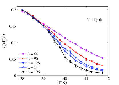
Figure 2: (color online) Ising order parameter(staggered magnetization)for double layer systems of different sizes across the zero-field AF-PM phase transition. Data with full dipolar interaction do not differ from those with only short range dipolar interaction.

Although the Ising order parameter shows a strong size dependence in the PM phase, the Neel temperature can not be determined directly from it. The Binder cumulant $U_{4}(M^{\dagger}_{z})$ is plotted in Fig. 3. Unlike the results in Ref. Lee et al., 2003, where the crossing points of $U_{4}$ are above all 40K, we see in Fig. 3 that all the crossing points are between 39.5K and 40K. The crossing points of these curves move up towards the universal value of the Ising universality class ($U_{4}^{*}\approx 0.618$) as the system size increases. This trend is more clearly revealed by curve fitting with smooth splines, shown in the inset of Fig. 3. Because data points for $\left<(M_{z}^{\dagger})^{4}\right>$ and $\left<(M_{z}^{\dagger})^{2}\right>$ have smaller error bars, we actually did a curve fitting for those two quantities first and plotted the Binder cumulant curve with the fitted functions. $T_{c}$ can be fixed to be between 39.5K and 39.6K, where the curves for three larger sizes cross. These observations suggest that the critical behavior of this dipolar two-dimensional Heisenberg antiferromagnet belongs to the Ising universality class. Therefore, we performed a finite size scaling analysis to test this prediction, as well as to fix the Neel temperature more accurately. Figure 4 shows the finite size scaling analysis of the Ising order parameter, where we plot $(T/T_{c}-1)L^{1/\nu}$ versus $\left<(M^{\dagger}_{z})^{2}\right>L^{2\beta/\nu}$, with Ising critical exponents $\nu=1$ and $\beta=1/8$ . Clearly, all the data from different sizes fall nicely on a single curve. The best result is achieved by choosing $T_{c}=39.56$K. Obvious deviations from a single curve are seen if $T_{c}$ changes by 0.1K, therefore we believe the error bar for $T_{c}$ is less than $0.1$K.

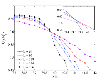
Figure 3: (color online) The Binder cumulant for the Ising order parameter across the AF-PM phase transition at zero field. The inset shows a smooth spline fitting of the original data. Crossing points in these curves approach the Ising universal value($\approx 0.618$).

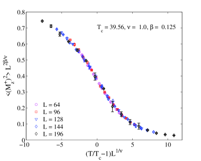
Figure 4: (color online) Finite size scaling analysis of the AF-PM phase transition at zero field. Data points are taken from Fig. 2. All of them fall onto a single curve with Ising critical exponents.

Although we have obtained a $T_{c}$ which is only slightly smaller than that obtained in Ref. Lee et al., 2003, our data for the Ising order parameter and its Binder cumulant are noticeably different from those in Ref. Lee et al., 2003. At the same temperature, data presented here are smaller than those in Ref. Lee et al., 2003. This difference is actually expected because of the difference in the strength of the dipolar interaction. The dipolar term is proportional to $S^{2}$ here in Eq. (1), but proportional to $S(S+1)$ in the previous work.

We have also performed simulations at $h=3$T and 5T to study the AF-PM phase transition in a finite magnetic field. The antiferromagnetic phase transition has been observed in both cases, but the order parameter changes more gradually with temperature when the magnetic field is turned on. Finite size scaling with Ising exponents have been performed. Figure 5 shows the scaling plot of $\left<(M_{z})^{2}\right>$ at $h=3$T, which has a lightly lower $T_{c}$. Long-range dipolar interaction only produces negligible changes in these data points. The valid regime for finite size scaling seems to be narrower than at $h=0$, because some deviations are clearly seen in the low-temperature data points. This could be due to the shape of the phase boundary, which is perpendicular to the temperature axis at $h=0$ by symmetry, but not so at a finite magnetic field. Because of this, we change both the temperature and the effective anisotropy when the simulation scans temperature at a constant magnetic field.

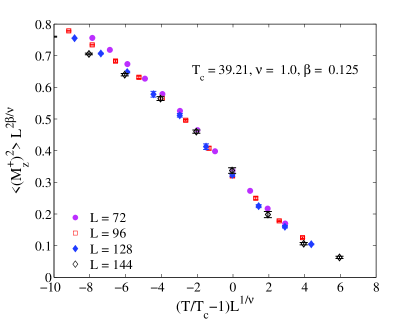
Figure 5: (color online) Same scaling plot as Fig. 4, but for simulations performed at $h=3$T. The critical temperature, at which the best collapsing of data points is achieved, is slightly lower than that of Fig. 4.

III.2 Kosterlitz-Thouless transition

When the magnetic field is above 6T, the AF-PM phase transition disappears. Instead, the XY order parameter Eq. (9) becomes large at low temperatures. For a two-dimensional anisotropic Heisenberg antiferromagnet, one expects to see an XY phase,Landau and Binder (1981); Holtschneider et al. (2005); Zhou et al. (2006) in which the correlation function decreases algebraically. Since the dipolar interaction breaks the spin rotational symmetry around the $z$ axis on a square lattice, one would expect the XY phase to be destroyed by its presence. In case of a ferromagnetic model, it has been shown that above a critical strength, the ferromagnetic dipolar XY model exhibits a ferromagnetic phase instead of an XY phase.Maier and Schwabl (2004) Experimentally, a “transverse” phase with long-range order has been found.Cowley et al. (1993) However, since the XY phase is also very sensitive to small perturbations such as crystal anisotropy and disorder, it is not clear whether the dipolar interaction in ${\rm Rb_{2}MnF_{4}}$ alone would prevent it from entering the XY phase. To answer this question, we performed simulations in constant magnetic fields $h=6.4,6.5$ and 7T at temperatures from 27K to 38K. Figure 6 shows the XY order parameter measured from these simulations for double layer systems with $L=72,96,128,144$, and 196.

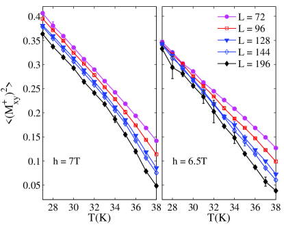
Figure 6: (color online) Average XY order parameter across the XY-PM phase boundary for double layer systems with different sizes.

In all these simulations, the XY order parameter increases gradually with lowering temperature in a broad range of temperature, and it is hard to determine the transition temperature from Fig. 6. They also look very different from the results in Ref. Holtschneider et al., 2005, where a transition in the XY order parameter from zero to a finite value is clearly visible. There are two reasons for this. First, the effective anisotropy induced by dipolar interaction in ${\rm Rb_{2}MnF_{4}}$ is very weak. The dipolar energy contributes only about 0.1 per cent to the total energy, while in the anisotropic Heisenberg model studied in Ref. Landau and Binder, 1981; Holtschneider et al., 2005; Zhou et al., 2006, the anisotropy is about 10 per cent to 20 per cent of the total energy (proportional to the anisotropy constant $\Delta$). Secondly, the magnetic field at which the simulations were performed (6.4T to 7T) is still close to the apparent spin-flop transition at about 6.2T, where the system is effectively an isotropic Heisenberg model. Experimentally, the existence of such an effective Heisenberg model has been tested.Christianson et al. (2001) Near the apparent spin-flop transition, the system has a large correlation length, which prevents the true XY critical behavior from being revealed in simulations of limited sizes. This also explains why in Fig. 6 $\left<(M_{xy}^{\dagger})^{2}\right>$ increases more rapidly at 7T with decreasing temperature than it does at 6.5T.

Nevertheless, we can see in Fig. 6 that the XY order parameter decreases with system size faster at higher temperatures than at lower temperatures. In the PM phase, one expects the size dependence to be exponential, i.e., $\left<(M_{xy}^{\dagger})^{2}\right>\propto\exp(-2L/\xi)$; while in the XY phase, the size dependence is power-law, i.e., $\left<(M_{xy}^{\dagger})^{2}\right>\propto L^{-2\eta}$, where $\eta$ is a temperature dependent exponent. On the XY-PM phase boundary, the critical value of this exponent is $\eta_{c}=1/8$. Therefore, we plot $\left<(M_{xy}^{\dagger})^{2}\right>$ versus $L$ in Fig. 7 with log-log scale, and try to identify the critical temperature for the Kosterlitz-Thouless transition.

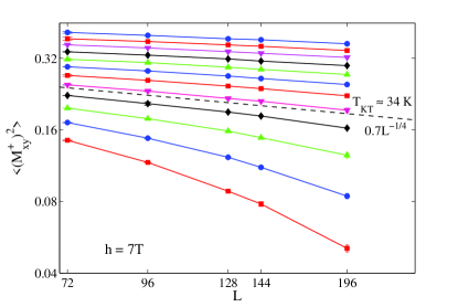
Figure 7: (color online) Log-log plot of the size dependence of the XY order parameter. The dashed line is a power-law with the critical exponent $2\eta_{c}=1/4$, used to identify the critical temperature. For each size, the temperatures of the data points are 27K, 28K,$\dots$, 38K from top to bottom.

Below the dashed line in Fig. 7, the order parameter obviously decreases faster than any power-law, which would be straight lines in the log-log scale. Above it, the data points are very close to power-law, and their slopes decrease with temperature. These features are consistent with an XY-PM phase transition. The critical temperature $T_{KT}$ is roughly 34K, estimated from Fig. 7. The same analysis has been done for simulations at $6.5$T and the estimated $T_{KT}$ is also near 34K.

It has been found that if the square anisotropy is strong, the XY model confirms the RG prediction that a second-order phase transition with nonuniversal critical exponents occurs.José et al. (1977); Rastelli et al. (2004a) If the anisotropy is weak, two possibilities for the phase diagram have been found by Monte Carlo simulations:Rastelli et al. (2004b) (1) a transition from the PM phase directly to the ferromagnetic phase, (2) a narrow XY phase is sandwiched between the ferromagnetic phase and the PM phase. Both of these cases might appear in our model if we replace the ferromagnetic phase with an antiferromagnetic phase. However, in all simulations performed above $h=6.4$T, at the lowest temperature $T=27$K, we still see that the XY order parameter decreases with increasing system size. No evidence for this phase is evident, at least for the range of lattice size that could be considered. Based on this observation we believe if a low temperature in-plane antiferromagnetic phase exists, it does not appear in the range of temperature and magnetic field where our simulations have investigated. Another check to exclude the transition from the PM phase to an Ising-like antiferromagnetic phase is to do the finite size scaling analysis with Ising exponents for the XY order parameter. We have found that it is impossible to collapse all the data points in Fig. 6 onto a single curve, no matter what critical temperature we use.

We have also performed simulations with a single layer of spins, and the results agreed with those for double layer systems within error bars. The results without perturbative reweighting, i.e., short-range dipolar interaction only, also do not differ noticeably from those with full dipolar interaction presented in Fig. 6 and 7. Therefore, we conclude that our results are consistent with an XY-PM transition. The main effect of the dipolar interaction is to provide an easy axis anisotropy, but the in-plane square anisotropy of the dipolar interaction is not strong enough to destroy the XY phase in the parameter ranges that we have examined.

III.3 The transition from AF phase to XY phase

Having found an Ising-like AF phase at low magnetic fields and an XY phase at high magnetic fields, we now turn to the boundary between these two phases. Precisely speaking, we want to tell if this boundary exists in the thermodynamic limit, and if it exists, find where it is connected to the XY-PM and AF-PM phase boundaries. So far, we know our system is best described by a two-dimensional anisotropic Heisenberg antiferromagnet with a very weak long-range interaction of square symmetry. Both the anisotropy and the long-range interaction come from the dipolar interaction. If the long-range component of the dipolar interaction can be completely ignored, the XY-PM phase boundary and the AF-PM phase boundary meet at a zero-temperature BCP, as predicted by RG theoryNelson (1976); Nelson and Pelcovits (1977) and confirmed by Monte Carlo simulations recently.Zhou et al. (2006) In this case, there is no real phase boundary between the XY phase and the AF phase. However, if the long-range component of the dipolar interaction is relevant, then the other two possibilities might be favored, i.e., a BCP at a finite temperature or a tetracritical point. In experiment, the neutron scattering data favored a finite temperature BCP, so that the transition from the AF phase to the “transverse” phase is a first order phase transition.Cowley et al. (1993) Whatever brings the transverse phase, which is observed to have long-range order, can also bring the bicritical point to a finite temperature. Because both the transverse phase and the AF phase have discrete symmetries, the BCP is not required to have a continuous (rotational) symmetry. The existence of such a bicritical point at finite temperature does not violate the Mermin-Wagner theorem.

We have performed simulations at constant temperatures $T=5,10,20$, and 30 K and calculated both the Ising order parameter and the XY order parameter for magnetic fields between 6T and 6.4T. We found that a transition apparently occurs at about 6.2T at all temperatures, and this transition happens over a larger range of magnetic field at higher temperatures than it does at lower temperatures. It must be pointed out that the location of this transition is about 0.9 to 1.1 T higher than the spin-flop transition in the experimental phase diagram. The transition field also does not show a noticeable temperature dependence, while the experimental spin-flop line has a positive slope. However, our result is in agreement with previous simulations in Ref. Lee et al., 2003, therefore we believe this difference is a result of the classical approximation we have adopted and also possibly some other weak effects, e.g., crystal field anisotropy, that we have not included in our simulations.

Figure 8 shows the Ising order parameter calculated at $T=20$K across the transition for different system sizes. The left panel shows the result calculated with only short-range dipolar interaction, and the right panel shows the same data reweighted with full dipolar interaction.

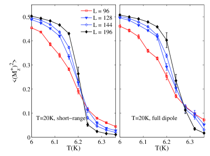
Figure 8: (color online) Ising order parameter of double layer systems across the apparent spin-flop transition at $T=20$K. The data reweighted with full dipolar interaction in the right panel shift towards large magnetic field, and have larger error bars.

The XY order parameter which becomes large in higher magnetic fields is shown in Fig. 9.

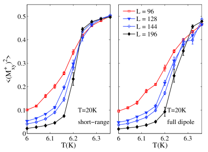
Figure 9: (color online) XY order parameter of double layer systems across the apparent spin-flop transition at $T=20$K. The data reweighted with full dipolar interaction in the right panel shift towards large magnetic field, and have larger error bars.

To tell if there is a BCP at a finite temperature, we need to classify the transition we have seen in Figs. 8 and 9 using a finite size scaling analysis. If it turns out to be a first order phase transition, a BCP must exist above 20K. The finite size scaling for the first order phase transition was established in Ref. Binder and Landau, 1984. For a BCP at $T=0$, Ref. Zhou et al., 2006 showed that logarithmic corrections to first order finite size scaling would be observed. We plot the Ising order parameter with the scaling ansatz for the zero-temperature BCP Zhou et al. (2006) in Fig. 10, and with the first order scaling ansatz in Fig 11.

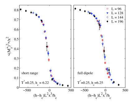
Figure 10: (color online) Finite size scaling plot of the Ising order parameter at $T=20$K with scaling ansatz for a zero-temperature BCP, where $x=1-T^{*}\ln L/(2\pi)$

In Fig. 10, we have two tunable parameters: the critical field $h_{c}$ and an effective temperature $T^{*}$. The logarithmic corrections, powers of $x=1-T^{*}\ln L/(2\pi)$, come from the spin renormalization constant calculated by RG for an effective anisotropic non-linear $\sigma$ model at $T^{*}$, with effective anisotropy vanishing at $h=h_{c}$. By tuning $h_{c}$ and $T^{*}$, we have collapsed all the data points with short-range dipolar interaction onto a single curve very well. The data with full dipolar interaction also collapse onto a single curve, except for a few data points with relatively large error bars. Especially on the low-field side of the figure, the quality of collapsing is good. On the other hand, the first order scaling plot in Fig. 11 shows clear systematic deviation in the low-field data points. This deviation is seen in both the left panel for short-range dipolar interaction and the right panel for full dipolar interaction. The only effect of the long-range part of the dipolar interaction is to shift the critical field $h_{c}$ up by 0.03T. Although this effect is small, it is clearly out of the error bars of the finite size scaling analysis. It is also expected from the comparison of left and right panels in Figs. 8 and 9, where the transition with the full dipolar interaction clearly shifts to higher magnetic fields.

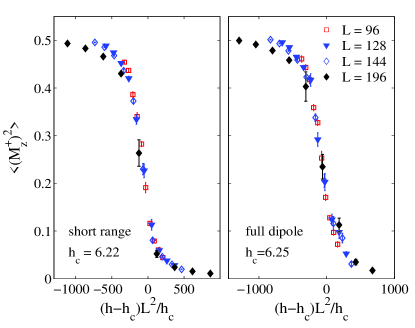
Figure 11: (color online) Finite size scaling plot of Ising order parameter at $T=20$K with scaling ansatz for a first order phase transition, to compare with Fig. 10.

The same scaling analysis applies to the XY order parameters as well. Figure 12 compares two finite size scaling plots for the XY order parameter at $T=20$K calculated with short-range dipolar interaction. Obviously the scenario of a zero-temperature BCP fits the data better than a first order phase transition.

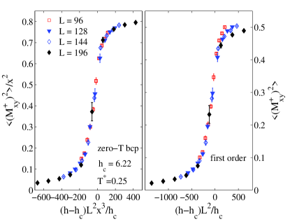
Figure 12: (color online) Finite size scaling of the XY order parameter at $T=20$K, comparison of first order scenario and zero-temperature BCP. The critical field $h_{c}$, and effective temperature $T^{*}$ are the same as those in Fig. 10.

At lower temperatures, the same scaling behavior of order parameters has been observed, and the critical field $h_{c}$ turns out to be nearly identical. Figure 13 shows the finite size scaling plots for Ising and XY order parameter calculated at $T=10$K. Since the transition at 10K happens within a narrower range of magnetic field, we have included data points reweighted at fields different than that of the simulation. Data points for $L=196$ close to the transition which have large error bars are reweighted with different magnetic fields. Nevertheless, most of the data points collapse nicely onto a single curve. For data with short-range dipolar interactions, we have again found $h_{c}=6.22$T; while for data reweighted with full dipolar interaction, the scaling plots look best if we choose $h_{c}=6.25$T.

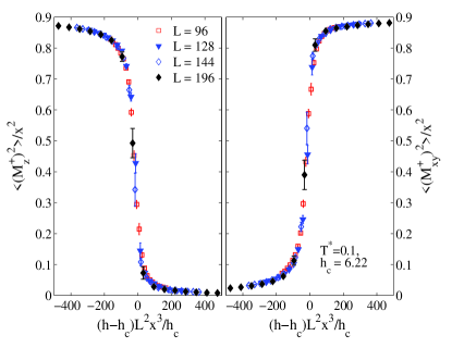
Figure 13: (color online) Finite size scaling of the Ising (left) and XY (right) order parameter calculated at 10K, corresponding to a zero-temperature BCP. Data shown here are calculated with short-range dipolar interaction for double layer systems, data with histogram reweighting at different magnetic are also shown. $h_{c}=6.22$ is the same as those in Fig. 10, while $T^{*}=0.1$ is smaller here.

Therefore, our finite size scaling so far is more consistent with a zero-temperature BCP than a finite temperature BCP above 20K. Reference Zhou et al., 2006 also predicts finite size scaling relations for the susceptibility and specific heat, it also predicts that the Binder cumulant $U_{4}(M^{\dagger}_{z})$ is close to, but slightly below, 0.4 at the critical field. We have observed the finite size scaling behavior of the susceptibility; however we have not seen behaviors of the Binder cumulant and the specific heat similar to those presented in Ref. Zhou et al., 2006. For the Binder cumulant, Fig. 14 shows that the curves for three larger sizes cross approximately at $h=6.203$T and $U_{4}=0.54$. This value is still very different from the universal value for the Ising universality class.

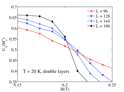
Figure 14: (color online) The Binder cumulant of the Ising order parameter, three curves for the larger sizes cross approximately at $h=6.203$T and $U_{4}=0.54$.

However, this is actually consistent with the theory in Ref. Zhou et al., 2006, if one notices that here we have two nearly independent layers of spins. If there is only one layer, Ref. Zhou et al., 2006 has shown that at the critical field, the system is effectively a single spin of length $\zeta$ with no anisotropy, where $\zeta$ is the spin renormalization constant. Its angular distribution is uniform, which implies $\left<(M_{z}^{\dagger})^{n}\right>=1/(n+1)$ and the crossing value of $U_{4}(M_{z}^{\dagger})$ is approximately 0.4. In our simulations, since we have more than one layer, and they are weakly coupled, we expect the total staggered magnetization of each layer ${\bf M}^{\dagger}_{l}$ is uniformly distributed on a sphere of radius $\zeta$. Due to our definition of $M^{\dagger}_{z}$ in Eq. (8), the distribution of $M^{\dagger}_{z}$ is not a uniform distribution, although $M^{\dagger}_{l,z}$ of each layer is distributed uniformly. Suppose the interlayer coupling can be completely ignored, which is a crude approximation. After some simple calculations, we found the probability distribution of $s=(M^{\dagger}_{z})^{2}/\zeta^{2}$ for a double layer system is

$$P(s)=\left\{\begin{array}[]{ll}{\pi\over 2},&0<s\leq{1\over 2},\\ \sin^{-1}{1\over\sqrt{2s}}-\sin^{-1}\sqrt{2s-1\over 2s},&1>s>{1\over 2}\end{array}\right..$$ (12)

Thus, if we ignore both the longitudinal fluctuation of staggered magnetization and the interlayer coupling, the Binder cumulant at the critical field should be $1-\left<s^{4}\right>_{P}/(3\left<s^{2}\right>_{P}^{2})$. A numerical evaluation of this expression gives 0.5334, which is very close to the crossing point in Fig. 14. Therefore, our simulation is consistent with weakly coupled multiple layers of an anisotropic Heisenberg antiferromagnet.

As for the specific heat, we have not seen a peak at the transition in all our simulations. Figure 15 shows the energy per spin and specific heat per spin calculated for double layer systems at $T=20$K with short range dipolar interaction. The energy drops when the magnetic field is larger than the critical field. However the specific heat shown in the inset does not show any sign of a peak. Although the error bar of the specific heat, as one can estimate from the fluctuation of the data points, is about 10 per cent, a peak which is expected to be similar to those discovered in Ref. Zhou et al., 2006, is clearly absent.

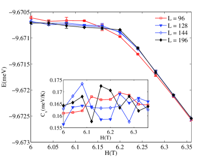
Figure 15: (color online) The average energy per spin for a double layer system at $T=20$K across the apparent spin flop transition. The inset shows the specific heat per spin, which does not show a peak similar to that of first or second order phase transitions.

However, this result is actually consistent with the finite size scaling theory for specific heat in Ref. Zhou et al., 2006, which shows that the peak in specific heat should be proportional to $(dh_{c}/dT)^{2}$. Because the critical field of our model is almost independent of the temperature, i.e., $dh_{c}/dT\approx 0$, we actually do not expect to see a peak in the specific heat here.

III.4 Discussions

To summarize our results, we construct a phase diagram in Fig. 16 based on our simulations and compare it to the experimental phase diagram from Ref. Cowley et al., 1993. Both our XY-PM and AF-PM phase boundaries are close to experimental results, the most pronounced difference is the spin-flop line. Rigorously speaking, our spin-flop line is not a single line, but the extensions of XY-PM and AF-PM phase boundaries which are exponentially close to each other and meet at a zero-temperature BCP. The experimental XY-AF “phase boundary” is empirical. Our spin-flop line is higher in magnetic field than the experimental one and has a nearly vanishing slope, but this difference in spin-flop field is most likely to be a consequence of the classical approximation which omitted quantum fluctuations of the spins. The anisotropic Heisenberg antiferromagnet studied in Ref. Zhou et al., 2006 offers an simple case to qualitatively analyze this effect. A brief derivation of the spin-flop field of this model is given in the appendix. If we assume the length of the classical spins is $\sqrt{S(S+1)}$, the zero-temperature spin-flop field of this simple model in the classical case is $4J\sqrt{S(S+1)(1-\Delta^{2})}$. The spin-flop field of the quantum mechanical Hamiltonian is found to be $4JS\sqrt{1-\Delta^{2}}$ within the linear spin-wave approximation. More accurate results can be obtained by quantum Monte Carlo simulations, however, the linear spin-wave theory has already considerably reduced the spin-flop field. Since this simple model and the dipolar Heisenberg antiferromagnet studied here have the same critical behavior near the apparent spin-flop transition, one would also expect the quantum effects in the latter model would reduce the spin-flop field by approximately the same amount. Acutally, given the classical result $h_{c}\approx 6.25$T, assuming the classical model consists of spins of length $\sqrt{S(S+1)}$, the reduced spin-flop transition would be $h_{c}/\sqrt{1+1/S}=5.28$T, which happens to be in agreement with the experimental value.

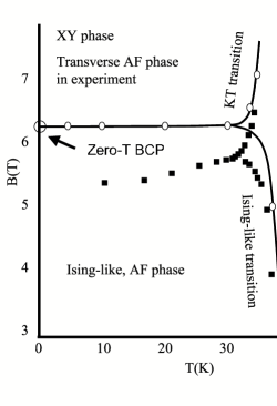
Figure 16: Comparison between our phase diagram and the experimental results. The experimental data points from Ref. Cowley et al., 1993 are ploted in solid squares.

Above the spin-flop line, we have observed the XY phase, as far as our simulations have covered, while the experiment shows a transverse phase. Therefore, our Hamiltonian certainly misses some weak but important effects in the real material, as the intricate correlation of the XY phase and the spin-flop transition is sensitive to many perturbations. Disorder is one of them, which can impose a cutoff in correlation length of the system so that the system would not approach the ideal zero-point BCP from the narrow PM phase. As a result, an apparent finite temperature BCP would be observed and the apparent spin-flop transition below the “BCP” looks like a first order transition. The disorder can come from both the crystal defects and slight inhomogeneity in the magnetic field. The experimentally observed finite temperature BCP can also be a result of crossover to three dimensions due to very weak exchange between layers.

The other facter that might have contributed to a phase diagram different from the experimental result is the exchange constant. The spin-wave analysis of $\rm Rb_{2}MnF_{4}$, which provided us the exchange constant $J$, were done for systems in zero magnetic field, and the dipolar interaction had already been simplified to a temperature dependent staggered magnetic field acting on Mn²⁺ spins.de Wijin et al. (1973) Therefore, the exchange integral provided by this theory is an effective quantity that depends on the particular form of the Hamiltonian which has been assumed. As far as we know, similar calculations have not been done in magnetic fields close to the spin-flop transition. It is not guaranteed that when the full dipolar interaction is used in the Hamiltonian, instead of an effective staggered magnetic field, the exchange integral deduced from a simplified Hamiltonian is still applicable and can be treated as a constant independent on either temperature or magnetic field.

Finally, we show some results that justify two main assumptions, i.e., the inclusion of only a few layers of Mn²⁺ spins, and the omission of two sublattices. Figure 17 shows the Ising order parameter across the apparent spin-flop transition for systems with $L=96$ but different number of layers. With short-range dipole interaction, the result seems to saturate when we have three or more layers. After reweighting with full dipolar interaction, the difference between data for different number of layers becomes even smaller. We estimate the change in $h_{c}$ due to the change in number of layers should be of order 0.01T. Therefore, it is justified to do simulations with only a few layers of spins. The crossover to a three dimensional system will only occur at very low temperatures.

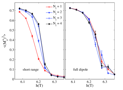
Figure 17: (color online) Ising order parameters calculated for systems at $T=10$K with $L=96$ and different number of layers. The thickness dependence is weak. It is more obvious in the left panel where we only include short-range dipolar interaction, than the right panel with full dipole reweighting.

Figure 18shows a finite-size scaling plot of the apparent spin-flop transition at $T=10$K calculated with two sublattices. The dipolar interactions between two sublattices were truncated to third nearest neighbors, i.e., an Mn²⁺ spin feels the magnetic field generated by totally 32 neighboring spins in the Mn²⁺ layer above and below it belonging to the other sublattice. The magnetic field contributed by spins outside this truncation radius should be extremely small based on our experience with the long-range dipolar interaction. Compared with Fig. 13, which was calculated with a single sublattice, the difference in $T^{*}$ and $h_{c}$ is negligible. We have enough reason not to expect the interaction between two sublattices to reduce the apparent spin-flop field $h_{c}$ by more than $0.1$T. The actual additional energy due to the inter-sublattice dipolar interaction is found to be only comparable to the long-range dipolar energy.

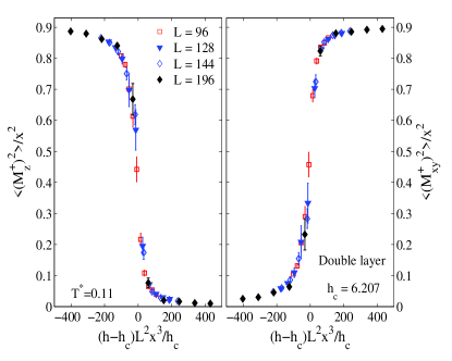
Figure 18: (color online) Finite-size scaling plot for simulations at $T=10$K with inter-sublattice dipolar interactions. The data in this figure only differ very slightly from those in Fig. 13, in which the inter-sublattice dipolar interactions were omitted.

IV Conclusions

In conclusion, we have tried to explain the phase diagram of $\rm Rb_{2}MnF_{4}$ using a classical spin model with dipolar interactions. A large amount of Monte Carlo simulations have been carried out to investigate the phase boundaries. Among different strategies to handle the dipolar interaction in the simulations, we have found our perturbative reweighting technique to be the most suitable for very weak dipolar interactions in $\rm Rb_{2}MnF_{4}$. The phase diagram inferred from our data captures the main features of the experimental phase diagram and the agreement is good at low magnetic fields. On the apparent spin-flop line, the XY and AF boundaries come so close together that they cannot be distinguished below an “effective” BCP at $T\approx 30$K. However, our data analyses support a zero temperature BCP. This conclusion is based on a novel finite size scaling analysis for two-dimensional anisotropic Heisenberg antiferromagnets.Zhou et al. (2006) If this multicritical point is located at very low finite temperature, as suggested by Ref. Pelissetto and Vicari, 2007. We believe its temperature must be sufficiently low, which is beyond our numerical accuracy. The ground state degeneracy for the anisotropic Heisenberg antiferromagnets as found in Ref. Holtschneider et al., 2007 may also exist in our model with dipolar interactions, which we have not yet verified. If it exists, one might simply rename the bicritical point as a tetracritical point. The zero temperature BCP is located above the experimental spin-flop line in the phase diagram, which appears to be a a line of first order phase transitions. We believe this difference from the experimental phase diagram is mainly caused by the classical approximation. Nevertheless, we have confirmed that the dominant effect of the dipolar interaction in $\rm Rb_{2}MnF_{4}$ is to provide an effective anisotropy, while other effects, such as in-plane square anisotropy and interlayer interaction, are extremely weak. Therefore, we would hope to obtain a more accurate phase diagram if we performed quantum Monte Carlo simulations for a simpler Hamiltonian which includes the effective anisotropy.

*

Appendix A Spin-flop field at $T=0$ of anisotropic Heisenberg antiferromagnet

As an analogy to the dipolar Heisenberg antiferromagnet, we consider the simple anisotropic Heisenberg antiferromagnet with the Hamiltonian:

$${\cal H}=J\sum_{\left<i,j\right>}\left[\Delta\left(S_{i}^{x}S_{j}^{x}+S_{i}^{y}S_{j}^{y}\right)+S_{i}^{z}S_{j}^{z}\right].-H\sum_{i}S_{i}^{z},$$ (13)

which is defined on a square lattice. The classical version of this model has been well studied,Landau and Binder (1981); Holtschneider et al. (2005); Zhou et al. (2006) where the spins are treated as unit vectors. The spin-flop field at zero-temperature is $H_{c}=4J\sqrt{1-\Delta^{2}}$. If we replace the spins with vectors of length $\sqrt{S(S+1)}$, $H_{c}$ is then modified to $4J\sqrt{S(S+1)(1-\Delta^{2})}$. This is not the only way to make connections to the quantum Hamiltonian. One can also replace $J$ with $JS(S+1)$, while replacing $H$ with $HS$, which can be justified by arguing that the Zeeman energy of the ferromagnetic configuration takes on the correct macroscopic value. In this case, the spin-flop field is modified to $H_{c}=4J(S+1)\sqrt{1-\Delta^{2}}$. However, in any case, we will show that the classical spin-flop field is larger than the quantum mechanical spin-flop field. By introducing the Holstein-Primakoff (HP) bosons on $A$ and $B$ sublattices respectively, and keeping the quadratic terms, the Hamiltonian Eq. (13) can be rewritten as

$${\cal H} \approx J\sum_{i\in A}\sum_{\left<j,i\right>}\left[\Delta S\left(a^{\dagger}_{i}b^{\dagger}_{j}+{\rm c.c.}\right)+(a^{\dagger}_{i}a_{i}-S)(S-b^{\dagger}_{j}b_{j})\right]$$ (14)

$$-H\sum_{i\in A}a^{\dagger}_{i}a+H\sum_{j\in B}b^{\dagger}_{i}b,$$

where $a$ and $a^{\dagger}$ are HP boson operators on sublattice $A$, $b$ and $b^{\dagger}$ on sublattice $B$, index $i$ labels sites on sublattice $A$ which are nearest neighbors of the sites on sublattice $B$ labeled with $j$. After a Fourier transformation, this quadratic Hamiltonian turns out to be

$${\cal H}=-4JS(S+1)N_{A}-HN_{A}-\sum_{{\bf k}}{\cal H}_{\bf k},$$ (15)

where $N_{A}$ is the number of sites on sublattice A, and

$${\cal H}_{\bf k}=SJ\left(\begin{array}[]{ll}a^{\dagger}_{\bf k}&b_{-{\bf k}}\end{array}\right)\left(\begin{array}[]{ll}4-h&\Delta\gamma_{{\bf k}}\\ \Delta\gamma_{{\bf k}}&4+h\end{array}\right)\left(\begin{array}[]{l}a_{\bf k}\\ b^{\dagger}_{-{\bf k}}\end{array}\right).$$ (16)

For simplicity, we have defined $h=H/SJ$ and $\gamma_{\bf k}=2\cos k_{x}+2\cos k_{y}$. The spin-wave spectrum can be obtained with the Bogoliubov transformation:

$$c_{\bf k}=\cosh\theta_{\bf k}a_{\bf k}+\sinh\theta_{\bf k}b^{\dagger}_{-\bf k},$$ (17)

$$d_{\bf k}=\sinh\theta_{\bf k}a^{\dagger}_{\bf k}+\cosh\theta_{\bf k}b_{-\bf k}.$$ (18)

In order to eliminate the cross terms in the Hamiltonian, one sets $\tanh 2\theta_{\bf k}=\Delta\gamma_{\bf k}/4$. Apart from a constant term, the spin-wave part of the Hamiltonian turns out to be

$${\cal H}_{\rm sw}=\sum_{\bf k}\left[\omega_{+}({\bf k})d^{\dagger}_{\bf k}d_{\bf k}+\omega_{-}({\bf k})c^{\dagger}_{\bf k}c_{\bf k}\right],$$ (19)

where

$$\omega_{\pm}({\bf k})=JS\sqrt{16-\Delta^{2}\gamma_{\bf k}^{2}}\pm H.$$ (20)

When $H$ is large enough such that $\omega_{-}(0)$ becomes negative, the AF ground state becomes unstable since the excitations on spin-wave mode $c_{{\bf k}=0}$ lower the ground state energy. This precisely indicates the the spin-flop instability. Therefore, the critical magnetic field is given by

$$H_{c}=4JS\sqrt{1-\Delta^{2}}.$$ (21)

Although the above spin-wave analysis is only a crude approximation, we see that the quantum effect lowers the spin-flop field by a factor of $S/(S+1)$ or $\sqrt{S/(S+1)}$, depending on which classical approximation one uses. The case with $\Delta=2/3$ and $S=1/2$ has been studied with quantum Monte Carlo simulations.Schmid et al. (2002) Its phase diagram shows the spin-flop field is at approximately $h/J_{xy}=1.8$, i.e., $H_{c}=1.2J$ in our notation here. The above spin-wave approximation gives $H_{c}=1.49J$, and the two classical approximations gives $H_{c}=4.47J$ and $H_{c}=2.58J$ respectively. Clearly, the classical approximations overestimate the spin-flop field. The difference from the real spin-flop field is large as we expect the quantum fluctuation to have a strong effect for $S=1/2$. For larger spins, such as $S=5/2$ which is studied in this paper, the classical approximation should work better. However, we still expect it to overestimate the spin-flop field by an noticeable amount.

References

- Kosterlitz et al. (1976) J. M. Kosterlitz, D. R. Nelson, and M. E. Fisher, Phys. Rev. B 13, 13 (1976).
- Nelson and Rudnick (1975) D. R. Nelson and J. Rudnick, Phys. Rev. Lett. 35, 178 (1975).
- Pelcovits and Nelson (1976) R. A. Pelcovits and D. R. Nelson, Phys. Letts. 57A, 23 (1976).
- Nelson (1976) D. R. Nelson, AIP Conf. Proc. 29, 450 (1976).
- Nelson and Pelcovits (1977) D. R. Nelson and R. A. Pelcovits, Phys. Rev. B 16, 2191 (1977).
- Landau and Binder (1978) D. P. Landau and K. Binder, Phys. Rev. B 17, 2328 (1978).
- Landau and Binder (1981) D. P. Landau and K. Binder, Phys. Rev. B 24, 1391 (1981).
- Holtschneider et al. (2005) M. Holtschneider, W. Selke, and R. Leidl, Phys. Rev. B 72, 064443 (2005).
- Zhou et al. (2006) C. Zhou, D. P. Landau, and T. C. Schulthess, Phys. Rev. B 74, 064407 (2006).
- Mermin and Wagner (1966) M. E. Mermin and H. Wagner, Phys. Rev. Lett. 17, 1133 (1966).
- Pelissetto and Vicari (2007) A. Pelissetto and E. Vicari, cond-mat/0702273 (2007).
- Holtschneider et al. (2007) M. Holtschneider, S. Wessel, and W. Selke, cond-mat/0703135 (2007).
- Birgeneau et al. (1970) R. J. Birgeneau, H. Guggenheim, and G. Shhirane, Phys. Rev. B 1, 2211 (1970).
- de Wijin et al. (1973) H. W. de Wijin, L. R. Walker, and R. E. Walstedt, Phys. Rev. B 8, 285 (1973).
- Christianson et al. (2001) R. J. Christianson, R. L. Leheny, R. J. Birgeneau, and R. W. Erwin, Phys. Rev. B 63, 140401(R) (2001).
- Lee et al. (2003) H. K. Lee, D. P. Landau, and T. C. Schulthess, J. Appl. Phys. 93, 7643 (2003).
- Breed (1967) D. J. Breed, Physica (Amsterdam) 37, 35 (1967).
- Cowley et al. (1993) R. A. Cowley, A. Aharony, R. J. Birgeneau, R. A. Pelcovits, G. Shirane, and T. R. Thurston, Z. Phys. B 93, 5 (1993).
- Ashcroft and Mermin (1976) N. W. Ashcroft and N. D. Mermin, Solid State Physics (Brooks Cole, 1976), chap. 32, p. 673.
- Lines (1967) M. E. Lines, Phys. Rev. 164, 736 (1967).
- Benson and Mills (1969) H. Benson and D. L. Mills, Phys. Rev. 178, 839 (1969).
- Costa Filho et al. (2000) R. N. Costa Filho, M. G. Cottam, and G. A. Farias, Phys. Rev. B 62, 6545 (2000).
- Wolff (1989) U. Wolff, Phys. Rev. Lett. 62, 361 (1989).
- Miyatake et al. (1986) Y. Miyatake, M. Yamamoto, J. J. Kim, M. Toyonaga, and O. Nagai, J. Phys. C 19, 2539 (1986).
- Loison et al. (2004) D. Loison, C. Qin, K. D. Schotte, and X. F. Jin, Ero. Phys. J. B 41, 395 (2004).
- Zhou et al. (2004) C. Zhou, M. P. Kennett, X. Wan, M. Berciu, and R. N. Bhatt, Phys. Rev. B 69, 144419 (2004).
- Ferrenberg and Swendsen (1988) A. M. Ferrenberg and R. H. Swendsen, Phys. Rev. Lett. 61, 2635 (1988).
- Landau and Binder (2000) D. P. Landau and K. Binder, A Guid to Monte Carlo Simulations in Statistical Physics (Cambridge University Press, 2000).
- Maier and Schwabl (2004) P. G. Maier and F. Schwabl, Phys. Rev. B 70, 134430 (2004).
- José et al. (1977) J. V. José, L. P. Kadanoff, S. Kirkpatrick, and D. R. Nelson, Phys. Rev. B 16, 1217 (1977).
- Rastelli et al. (2004a) E. Rastelli, S. Regina, and A. Tassi, Phys. Rev. B 69, 174407 (2004a).
- Rastelli et al. (2004b) E. Rastelli, S. Regina, and A. Tassi, Phys. Rev. B 70, 174447 (2004b).
- Binder and Landau (1984) K. Binder and D. P. Landau, Phys. Rev. B 30, 1477 (1984).
- Schmid et al. (2002) G. Schmid, S. Todo, M. Troyer, and A. Dorneich, Phys. Rev. Lett. 88, 167208 (2002).