FERMILAB-PUB-07-136-T

CLNS 06/1966

Radion Phenomenology in Realistic Warped Space Models

Csaba Csáki^a, Jay Hubisz^b, and Seung J. Lee^a

^a Institute for High Energy Phenomenology
Newman Laboratory of Elementary Particle Physics
Cornell University, Ithaca, NY 14853, USA

^b Fermi National Accelerator Laboratory
P.O. Box 500, Batavia, IL 60510, USA

csaki@lepp.cornell.edu, hubisz@fnal.gov, sjl18@cornell.edu

We investigate the phenomenology of the Randall-Sundrum radion in realistic models of electroweak symmetry breaking with bulk gauge and fermion fields, since the radion may turn out to be the lightest particle in such models. We calculate the coupling of the radion in such scenarios to bulk fermion and gauge modes. Special attention needs to be devoted to the coupling to massless gauge fields (photon, gluon), since it is well known that loop effects may be important for these fields. We also present a detailed explanation of these couplings from the CFT interpretation. We then use these couplings to determine the radion branching fractions and discuss some of the discovery potential of the LHC for the radion. We find that the $\gamma\gamma$ signal is enhanced over most of the range of the radion mass over the $\gamma\gamma$ signal of a SM Higgs, as long as the RS scale is sufficiently low. However, the signal significance depends strongly on free parameters that characterize the magnitude of bare brane-localized kinetic terms for the massless gauge fields. In the absence of such terms, the signal can be be enhanced over the traditional RS1 models (where all standard model fields are localized on the IR brane), but the signal can also be reduced compared to RS1 if the brane localized terms are sizeable. We also show that for larger radion masses, where the $\gamma\gamma$ signal is no longer significant, one can use the usual 4 lepton signal to discover the radion.

1 Introduction

There has been a lot of attention devoted to models of physics above the weak scale utilizing warped extra dimensions. The first proposal [1] of Randall and Sundrum (RS1) solves the hierarchy problem by localizing all standard model (SM) particles on the IR brane. Much research has been done on understanding possible mechanisms for radius stabilization and the phenomenology of the radion field in this model [2, 3, 4, 5, 6, 7, 8]. The motivation for studying the radion is twofold. First, the radion may turn out to be the lightest new particle in the RS-type setup, possibly accessible at the LHC. In addition, the phenomenological similarity and potential mixing of the radion and the Higgs boson warrant detailed study in order to facilitate distinction between radion and Higgs signals at colliders.

By now it is quite clear that, in order to make a realistic model of electroweak symmetry breaking (EWSB) in an RS-type scenario, the model needs to be modified by extending the gauge fields and fermions into the bulk. This is forced by constraints from flavor physics and electroweak precision tests of the SM. Since the cutoff scale on the IR brane is of the order of a few TeV, one would expect dimension 6 operators localized on the TeV brane to be suppressed by this relatively low scale, giving unacceptably large corrections to electroweak precision observables such as the T-parameter, and also to flavor changing neutral currents. Another way to see this is to invoke the AdS/CFT correspondence [9, 10, 11]. The conformal field theory (CFT) interpretation of the 2-brane RS1 model is a 4D CFT that is spontaneously broken at the TeV scale. At the scale of conformal symmetry breaking, the broken CFT produces a SM where all of the fields are composites, and since the scale of compositeness is low one would again expect large corrections to precision observables.

In order to overcome this problem first the gauge fields were moved to the bulk [12], but $S$ and $T$ still remained large [13]. A more realistic approach can be found by moving both gauge fields and fermions into the bulk, and incorporating a custodial symmetry [14]. Variations of this basic setup include Higgsless models (with boundary condition EWSB) [15] and holographic composite Higgs models [16].

While the gauge and matter sector model building has advanced tremendously, little attention has been paid to the modification of the radion physics due to the change in the model structure (with the exception of [17]). The aim of this paper is to lay down the groundwork for finding the basic properties of the radion in one of these realistic warped EWSB models. In Sec. 2 we review the radion mode and the general expression for its tree level coupling. In Sec. 3 we find the couplings to bulk fermions, including those localized on the UV and IR branes. In Sec. 4 we investigate the couplings to gauge bosons. Particular attention needs to be paid to massless gauge bosons, since some of the calculable one-loop contributions turn out to be important. This has to be investigated carefully, since important production and discovery channels at the LHC include couplings to massless gauge fields. In Sec. 5 we review the CFT interpretation of the radion and use this to re-derive the various couplings to massive and massless fields. In Sec. 6 we present the branching fractions of the radion as a function of the parameters of the 5D model, while in Sec. 7 we show some of the possible discovery channels at the LHC. We conclude in Sec. 8, and present Appendices clarifying the role of boundary kinetic terms for fermions, the CFT interpretation of fermion masses for bulk fields, and an explicit 5D loop calculation illustrating that renormalization of the brane induced gauge kinetic terms captures the leading one loop effects of the radion coupling to massless gauge bosons.

2 The radion solution

Throughout this paper, we use the conventions of [6, 18]. The $z$ coordinate will always refer to the conformally flat AdS background with $R<z<R^{\prime}$, and the AdS curvature is $R=1/k$, while the $y$ coordinates are given by $y=R\log z/R$. The AdS metric including the scalar perturbation $F$ corresponding to the effect of the radion is given in these coordinate systems by

$$ds^{2}=e^{-2(A+F)}\eta_{\mu\nu}-(1+2F)^{2}dy^{2}=\left(\frac{R}{z}\right)^{2}\left(e^{-2F}\eta_{\mu\nu}dx^{\mu}dx^{\nu}-(1+2F)^{2}dz^{2}\right),$$ (2.1)

where $A(y)=k\,y$. Note that the perturbed metric is no longer conformally flat, even in $z$ coordinates. At linear order in the flutuation, $F$, the metric perturbation is given by

$$\delta(ds^{2})\approx-2F\left(e^{-2A}\eta_{\mu\nu}dx^{\mu}dx^{\nu}+2~{}dy^{2}\right)=-2F\left(\frac{R}{z}\right)^{2}\left(\eta_{\mu\nu}dx^{\mu}dx^{\nu}+2dz^{2}\right).$$ (2.2)

In the absence of a stabilizing mechanism, the radion is precisely massless, however it was shown that the addition of a bulk scalar field with a vacuum expectation value (vev) leads to an effective potential for the radion after taking into account the back-reaction of the geometry due to the scalar field vev profile [2]. In our analysis that follows, we assume that this backreaction is small, and does not have a large effect on the 5D profile of the radion.

The radion is assumed to take the form $F(x,z)=r(x){\rm R}(z)$, where the form of $R(z)$ is determined by imposing that the metric solve Einstein’s equations, and that $r(x)$ be a canonically normalized 4D scalar field after integrating out the extra dimension.

In the limit of small back-reaction, the relation between the canonically normalized 4D radion field $r(x)$ and the metric perturbation $F(z,x)$ is given by

$$F(z,x)=\frac{1}{\sqrt{6}}\frac{R^{2}}{R^{\prime}}\left(\frac{z}{R}\right)^{2}r(x)=\frac{r(x)}{\Lambda_{r}}\,\left(\frac{z}{R^{\prime}}\right)^{2},$$ (2.3)

with

$$\Lambda_{r}\equiv\frac{\sqrt{6}}{R^{\prime}}.$$ (2.4)

In order to find the interaction terms between the radion and the SM fields to linear order in the radion, we can use the fact that the energy momentum tensor of the matter fields is just the linear variation of the action with respect to the metric, thus

$$S_{\mathrm{radion}}=-\frac{1}{2}\int d^{5}x\sqrt{g}T^{MN}\delta g_{MN}.$$ (2.5)

Plugging in for the expression for $\delta g_{MN}$ corresponding to the radion fluctuation from Eq. (2.2), we find the interactions of the radion are given by

$$S_{\mathrm{radion}}=\int d^{5}x\sqrt{g}\left[F\left(\mathrm{Tr~{}}T^{MN}-3T^{55}g_{55}\right)\right].$$ (2.6)

Note that the radion couples to a 5D scale invariant object, which can be thought as an effective 4D trace when integrated over the z-direction. If all the SM fields are localized on the IR brane, these become the radion interactions of the RS1 model, $\frac{r}{\Lambda_{r}}\,T^{\mu}_{\,\mu}$, which is proportional to the 4D trace of the brane localized energy-momentum tensor [2, 3, 4, 5, 6, 7, 8].

3 Radion Couplings to Fermions

The 5D action for bulk fermions can be written as

$$S=\int d^{5}x\sqrt{g}\left(\frac{i}{2}(\bar{\Psi}\,\Gamma^{M}D_{M}\Psi-D_{M}\bar{\Psi}\,\Gamma^{M}\Psi)+m\bar{\Psi}\Psi\right),$$ (3.1)

where $\Psi$ is the 5D Dirac spinor, and M=0,1,2,3,4,5. Here the $\Gamma$ matrices are given by $\Gamma^{M}=\gamma^{a}e^{M}_{a}$, where the $\gamma^{a}$ are the ordinary $\gamma$-matrices with $\gamma^{5}=i{\rm diag}(1_{2},-1_{2})$, and the 5D vielbein defined by $e^{M}_{a}e^{N}_{b}\eta^{ab}=g^{MN}$ is given for the metric including the radion fluctuation (to linear order in $F$) by

$$e^{M}_{a}={\rm diag}\frac{z}{R}(1+F,1+F,1+F,1+F,1-2F).$$ (3.2)

The covariant derivative is given by $D_{M}=\partial_{M}+\frac{1}{2}\omega_{bcM}\sigma^{bc}$ where the $\omega$’s are the spin connections. This action can be also written as

$$S=\int d^{5}x\sqrt{g}\left(e^{M}_{a}\frac{i}{2}(\bar{\Psi}\,\gamma^{a}\partial_{M}\Psi-\partial_{M}\bar{\Psi}\,\gamma^{a}\Psi+\omega_{bcM}\bar{\Psi}\frac{1}{2}\{\gamma^{a},\sigma^{bc}\}\Psi)+m\bar{\Psi}\Psi\right).$$ (3.3)

The advantage of writing the action in this form is that one can show that the contribution involving the spin connections will be vanishing for diagonal metrics (and vielbeins), as in our case.

In order to find the interaction of fermions with the radion we expand this action to linear order in $F$. We first separate the bulk Dirac fermion into two component spinors as

$$\Psi=\left(\begin{array}[]{c}\chi_{\alpha}\\ \bar{\psi}^{\dot{\alpha}}\end{array}\right),$$ (3.4)

where $\chi$ is the left handed spinor and $\bar{\psi}$ is the right handed. For their interactions with the radion we find (introducing the usual notation $c=mR$):

$$\frac{r}{\sqrt{6}}\frac{R^{2}}{R^{\prime 2}}\int dz\left(\frac{R}{z}\right)^{2}\left[-i(\psi\sigma^{\mu}\partial_{\mu}\bar{\psi}+\bar{\chi}\bar{\sigma}^{\mu}\partial_{\mu}\chi)+2(\psi\overleftrightarrow{\partial_{5}}\chi-\bar{\chi}\overleftrightarrow{\partial_{5}}\bar{\psi})+\frac{2c}{z}(\psi\chi+\bar{\chi}\bar{\psi})\right].$$ (3.5)

We are interested in the interaction terms between the 4D Kaluza-Klein (KK) modes of the fermions with the radion. The KK decomposition is, as usual, given by

$$\chi_{=}\sum_{n}g^{n}(y)\,\chi^{n}(x),$$ (3.6)

$$\bar{\psi}=\sum_{n}f^{n}_{i}(y)\,\bar{\psi}^{n}(x).$$ (3.7)

where $\chi^{n}(x)$ and $\bar{\psi}^{n}(x)$ are four dimensional spinors satisfying the 4D Dirac equation

$$-i\bar{\sigma}^{\mu}\partial_{\mu}\chi_{n}+m_{n}\,\bar{\psi}_{n}=0,$$ (3.8)

$$-i\sigma^{\mu}\partial_{\mu}\bar{\psi}_{n}+m_{n}\,\chi_{n}=0.$$ (3.9)

Using this, Eq. (3.5) can be rewritten as

$$\frac{r}{\sqrt{6}}(\psi_{n}\chi_{n}+\bar{\chi}_{n}\bar{\psi}_{n})\int dz\left(\frac{R}{z}\right)^{2}\frac{R^{2}}{R^{\prime}}\left[-\frac{m_{n}}{2}\left(f_{n}^{2}+g_{n}^{2}\right)+2(f_{n}g_{n}^{\prime}-f_{n}^{\prime}g_{n}+\frac{c}{z}f_{n}g_{n})\right],$$ (3.10)

where we have assumed that the two fermions coupling to the radion are at the same level in the KK tower. It is easy to extend this formula to calculate the coupling of the radion to two different KK mode fermions, but for the purposes of this paper we are most interested in the couplings of the radion to the SM fermions (the lightest elements of the KK tower). In this case, Eq. (3.10) is sufficient.

One subtlety that one needs to clarify is the effect of adding brane localized interactions for the fermions. First, boundary mixing of bulk fermions is what normally leads to masses for the SM fermions, so in general, Eq. (3.10) must be summed over all bulk fermions that mix to form the mass eigenstates. In addition, it appears naively that localized mass terms will also give a direct contribution to the coupling. However, in Appendix A we show that a careful treatment of the boundary conditions implies that the contributions from the localized terms actually cancel against the induced wave function discontinuity contributions to the stress-energy tensor at the TeV brane. Thus Eq. (3.10) is the full expression for the fermion-radion coupling.

3.1 Approximate radion couplings to fermions in a simplified model of fermion masses

In order to evaluate the expression (3.10) we need to understand the basic properties of the mechanism responsible for generating the fermion masses. We consider the radion coupling to fermions in the simple example of a bulk SU(2)${}_{L}\times$U(1)_Y gauge group with the usual SM quantum number assignments for the bulk Dirac fermions. The boundary conditions will then be chosen such that from the SU(2)_L doublets the left handed ($\chi$) fermions have zero modes, while from the singlets it is the right handed ($\psi$) fermions that have zero modes. If we denote the SU(2) doublet fields as L-fields and the singlet fields as R-fields, then the BC’s providing the proper zero modes are $\psi_{L}|_{z=R,R^{\prime}}=\chi_{R}|_{z=R,R^{\prime}}=0$. In this simple model, the electroweak symmetry is broken via the Higgs, which is localized on the TeV brane, and which generates masses for the zero modes. The localized Higgs will generate a TeV-brane localized Dirac mass: $M_{D}R^{\prime}\bar{\Psi}_{L}\Psi_{R}$. In this model, for every fermion there are bulk mass parameters $c_{L}$ for the doublets and a separate $c_{R}$ for every right handed field which characterize the profiles of the zero modes. With the conventions used in this paper, the wave functions of the fermions are localized on the Planck brane for $c_{L}>1/2$ (and for $c_{R}<-1/2$), while in the opposite case they are localized on the TeV brane. In addition there is a separate Dirac mass term $M_{D}$ for every fermion.

The radion coupling to SM fermions should be proportional to the physical mass of this field. Generically, these lowest lying modes are considerably lighter than the scale $1/R^{\prime}$, making it useful to find the radion-fermion coupling as an expansion in $mR^{\prime}$. The expression for the lightest eigenvalue is found to be:

$$m^{2}=M_{D}^{2}\frac{(1+2c_{R})(1-2c_{L})}{\left(1-\lambda^{1+2c_{R}}\right)\left(1-\lambda^{1-2c_{L}}\right)},$$ (3.11)

where we have defined $\lambda\equiv R/R^{\prime}$. The light fermions are usually assumed to be localized around the Planck brane ($c_{L}>1/2,c_{R}<-1/2$). For this case, the coupling in Eq. (3.10) simplifies to

$$\frac{r}{\Lambda_{r}}m(c_{L}-c_{R})$$ (3.12)

after summing over the bulk L and R fields.

Note that, for the light fermions, the interactions with the radion depend on the bulk profiles. In order for the top to be sufficiently heavy we need to assume that its wave function is localized on the TeV brane, that is $c_{L}<1/2$ and $c_{R}>-1/2$. As expected for this TeV brane localized case, the leading coupling is equal to the usual result from the brane localized mass terms in the RS1 model, and is insensitive to the bulk mass parameters:

$$\frac{r}{\Lambda_{r}}m.$$ (3.13)

3.2 Radion coupling to fermions in models with custodial SU(2)

Realistic models of EWSB with bulk fermions need to incorporate a custodial SU(2) symmetry in order to protect the $T$-parameter from large corrections. This is achieved by gauging SU(2)${}_{L}\times$SU(2)${}_{R}\times$U(1)_B-L in the bulk of AdS₅, and then breaking SU(2)${}_{L}\times$SU(2)${}_{R}\to$SU(2)_D on the TeV brane either via a localized Higgs or boundary conditions, while on the Planck brane SU(2)${}_{R}\times$U(1)${}_{B-L}\to$U(1)_Y. This setup has been first suggested in [14] for RS-type models, and applied to Higgsless models in [15]. This implies a modification of the model of fermion masses discussed in the previous section. The simplest possibility is to put the two right handed bulk fields into a doublet of SU(2)_R. Similar to the previous case without custodial SU(2), the zero modes obtained from the orbifold projections will pick up a mass once a Dirac mass term $M_{D}\bar{\Psi}_{L}\Psi_{R}$ is added on the TeV brane. In order to split the up and down type quarks (and the charged leptons from the neutrinos) one can either introduce a brane kinetic term (BKT) for the R-fields on the Planck brane or, for the neutrinos, a Majorana mass for the right handed component. The parameters of this model are: $c_{L},c_{R},M_{D}$ and a parameter $\alpha$ characterizing the size of the Planck brane induced kinetic term for the SU(2)_R fields (or $M_{M}$ for a RH neutrino Majorana mass).

Another possible model for the fermion masses with custodial SU(2) is to introduce a separate SU(2)_R doublet for every SM field. In this case the correct chiral spectrum is obtained by assigning the following parities:

• $(+,+)$ for $\chi_{L},\psi_{u_{R}}$ and $\tilde{\psi}_{d_{R}}$

• $(-,-)$ for $\psi_{L},\chi_{u_{R}}$ and $\tilde{\chi}_{d_{R}}$

• $(+,-)$ for $\chi_{d_{R}}$ and $\tilde{\chi}_{u_{R}}$

• $(-,+)$ for $\psi_{d_{R}}$ and $\tilde{\psi}_{u_{R}}$

In this case one can add a separate Dirac mass on the TeV brane mixing the left handed doublet with either of the right handed ones. A mixing term between the right handed fields (which would be allowed by the gauge quantum numbers) is vanishing due to the parity assignments. In this case the parameters of the model are one $c_{L}$ and a separate $c_{R}$ for every SU(2)_R field, and a separate Dirac mass on the TeV brane. Thus the parameters in this model actually match the parameters in the model without custodial SU(2) symmetry.

We can again evaluate the approximate expression for the fermion-radion coupling for both of these models. For the case of the model with the three multiplets the general expression for the coupling is given by

$$\frac{r}{\Lambda_{r}}m\frac{c_{R}-c_{L}+\frac{1}{2}(1-2c_{R})\lambda^{2c_{L}-1}-\lambda^{2c_{L}-2c_{R}-2}}{(1-\lambda^{2c_{L}-1})(1-\lambda^{-1-2c_{R}})}.$$ (3.14)

For the case relevant for the light fermions we get the same approximate expression (3.12) as in the simple model and similarly for the case relevant to the top quark we find (3.13). However, for the bottom quark (assuming $c_{L}<1/2,-0.68<c_{R}<-1/2$) we find a coupling given by

$$\frac{r}{\Lambda_{r}}\frac{m}{2}(2c_{R}-1).$$ (3.15)

One can check that, to leading order in the masses, the same approximate expressions apply in the model with just two bulk fermions where there are Planck brane localized kinetic terms for the SU(2)_R fields.

4 Radion couplings to gauge bosons

We expect to find the most important effects in this sector. The reason is that once the gauge field is a(n approximate) bulk zero mode its wave function is not peaked on the TeV brane, so there is no limit in which this setup reproduces the naive RS1 model. This will result in the main new effect: the existence of tree level couplings of the radion to the bulk kinetic terms of the gauge bosons. For the massive gauge bosons, the coupling proportional to the mass is dominant over the new kinetic term coupling. For massless gauge bosons, however, the tree level coupling to the field strength squared is often the dominant effect, and one has to add the effects from the bulk and brane localized kinetic terms.

4.1 Radion couplings to massive gauge bosons

First we consider the simpler case of massive gauge bosons. Just as in the case of fermion couplings, we treat the Higgs as completely localized on the IR brane. The action for the massive gauge bosons is then given by

$$S_{\mathrm{W}}=\int\sqrt{g}\Big{(}-\frac{1}{2}g^{MN}g^{KL}W^{\dagger}_{MK}W_{NL}+g^{\mu\nu}\frac{\delta(z-R^{\prime})}{\sqrt{g_{55}}}\,\left(g_{5}\,v\right)^{2}W_{\mu}^{\dagger}W_{\nu}\Big{)},$$ (4.1)

and

$$S_{\mathrm{Z}}=\int\sqrt{g}\Big{(}-\frac{1}{4}\,g^{MN}g^{KL}Z_{MK}Z_{NL}+\frac{1}{2}\,g^{\mu\nu}\frac{\delta(z-R^{\prime})}{\sqrt{g_{55}}}\,(\sqrt{g_{5}^{2}+{g^{\prime}_{5}}^{2}}\,v)^{2}Z_{\mu}Z_{\nu}\Big{)},$$ (4.2)

where $v$ is the localized Higgs vev, which can be different from the SM vev in two ways: first, one needs to rescale by the usual RS warp factor in AdS space, second, in principle a large fraction of the gauge boson mass could arise from the bulk curvature of the gauge boson wave functions as in Higgsless models. In either case, the dominant couplings to the radion are given by:

$${\cal{L}}=-\frac{r}{\Lambda_{r}}\,\left(2M^{2}_{W}\,W^{+}_{\mu}\,W^{\mu-}+M_{Z}^{2}Z_{\mu}\,Z^{\mu}\right).$$ (4.3)

If the $W,Z$ masses come from a localized Higgs vev, the corrections to the coupling in Eq. (4.3) are then given by

$$-\frac{r}{4\Lambda_{r}\log{\frac{R^{\prime}}{R}\,}}(2W^{\dagger}_{\mu\nu}W^{\mu\nu}+Z_{\mu\nu}Z^{\mu\nu})+\frac{M_{W}^{4}\,R^{\prime 2}}{\Lambda_{r}}\,\log{\frac{R^{\prime}}{R}\,}r\,W_{\mu}\,W^{\mu}+\frac{M_{Z}^{4}\,R^{\prime 2}}{2\Lambda_{r}}\,\log{\frac{R^{\prime}}{R}\,}r\,Z_{\mu}\,Z^{\mu},$$ (4.4)

where we have used the wave function for the $W$ boson given in [13]:

$$W^{\mu}(z,x)\simeq\frac{1}{\sqrt{R\log{\frac{R^{\prime}}{R}\,}}}\,\Big{(}1+\frac{M_{W}^{2}}{4}\,(z^{2}-R^{\prime 2}-2z^{2}\log{\frac{R^{\prime}}{R}\,}+2R^{\prime 2}\log{\frac{R^{\prime}}{R}\,})\Big{)}W^{\mu}(x).$$ (4.5)

A similar formula applies for the $Z$ boson. We have assumed that there are no BKTs for the $W$ and $Z$. Note that these corrections are dependent on the specifics of EWSB, and will be different, for example, in Higgsless models of EWSB. The coupling to the field strengths in the first term of Eq. (4.4) is a new feature of bulk RS gauge fields that plays a significant role only for momentum transfer well above the electroweak mass scale.

4.2 Radion couplings to the massless gauge bosons

For the massless gauge bosons, there is no large coupling to the radion as there are no brane localized mass terms. In order to take potentially large loop effects into account we also consider brane localized kinetic terms for the gauge fields. The action for the massless gauge boson is then given by (note that, for this discussion, is it convenient to use non-canonically normalized gauge fields)

$$S_{\mathrm{massless}}=-\frac{1}{4g_{5}^{2}}\int d^{5}x\sqrt{g}F_{MN}F^{MN}-\frac{1}{4}\int d^{4}x\sqrt{g_{UV,IR}}\tau_{UV,IR}F_{\mu\nu}F^{\mu\nu}$$ (4.6)

where $F$ is either the photon or the gluon, and $\tau_{UV},\tau_{IR}$ parameterize the Planck and TeV brane induced kinetic terms. With this definition, the tree-level matching relation between the 4D and 5D couplings is given by [22, 23, 24, 25, 26]

$$\frac{1}{g_{4}^{2}}=\frac{R\log\frac{R^{\prime}}{R}}{g_{5}^{2}}+\tau_{UV}+\tau_{IR}$$ (4.7)

Plugging in the gauge boson and radion wave functions, we find that the bulk contribution to the coupling is

$$-\frac{R}{R\log{\frac{R^{\prime}}{R}\ +(\tau_{UV}+\tau_{IR})g_{5}^{2}}}\frac{r}{4\Lambda_{r}}F_{\mu\nu}F^{\mu\nu}=-\frac{Rg_{4}^{2}}{g_{5}^{2}}\frac{r}{4\Lambda_{r}}F_{\mu\nu}F^{\mu\nu}.$$ (4.8)

Note that the above expression gets a direct contribution only from the bulk, since the induced 4D kinetic terms are scale invariant at tree level. This formula already incorporates some of the one-loop corrections as well: it contains the loop effects corresponding to the renormalization of the local 5D operators (bulk + brane localized kinetic terms). In particular, potentially large linearly divergent contributions to the radion coupling from one-loop bulk gauge coupling renormalization and bulk triangle diagrams vanish (as we show in Appendix C) after assuming appropriate bulk counterterms and using the renormalized values for the bulk and brane localized parameters. In addition there can be brane localized direct contributions to the radion-gauge boson coupling which we will discuss, and possible (subleading) non-local effects which we neglect.

We now add the effect of the localized trace anomalies and of loop induced couplings due to the zero modes. There are no large loop induced bulk couplings. The reason for this is that in the bulk there is a tree level coupling between the radion and the gauge fields. Therefore loop effects merely renormalize this tree level operator. On the branes, there is no allowed tree level coupling, thus the loop effects are finite and have to be included separately. Since the wave function of the radion is negligible on the UV brane, we only add the effects on the IR brane. The localized trace anomaly on the IR brane is exactly the same effect as the entire radion coupling to massless gauge bosons in the original RS1 model, as studied in [4], except we need to add it only for the fields that are localized on the IR brane. Thus the coupling due to the localized trace anomaly will be

$$-\frac{r}{\Lambda_{r}}\frac{b_{IR}\alpha}{8\pi}F_{\mu\nu}F^{\mu\nu}.$$ (4.9)

where $b_{IR}$ is the $\beta$-function coefficient of the light fields localized on the IR brane. In our case these are the top quark pair $\left(t_{L},\,t_{R}\right)$, left-handed bottom quark $\left(b_{L}\right)$ and the Higgs. Thus for the gluon $b^{3}_{IR}=b^{3,t_{L}}+b^{3,t_{R}}+b^{3,b_{L}}=-1$, while for the photon $b^{EM}_{IR}=b^{EM,H}+N_{c}b^{EM,t_{L}}+N_{c}b^{EM,t_{R}}+N_{c}b^{EM,b_{L}}=-7/3$.

Figure 1: Triangle diagrams

In addition, there are triangle diagrams, as shown in Fig1, involving either the gauge fields, the Higgs or the top quark that introduce a finite contribution to the coupling. We calculate this in the low energy effective 4D theory. This is again the analog of the effect of the straight RS1 contribution as explained in [4]. Noting that the leading contributions to the couplings to heavier fields, such as $W$ and top, are the same as in the RS1 model, the loop induced brane localized coupling due to the top quark is given by

$$\mu_{t}F_{1/2}(\tau_{t})\frac{\alpha}{8\pi}\frac{r}{\Lambda_{r}}F_{\mu\nu}F^{\mu\nu}$$ (4.10)

where $\mu_{t}=1/2$ for the gluon and $Q_{t}^{2}$ for the photon. In this expression $\tau_{t}=4(m_{t}/m_{r})^{2}$, and $F_{1/2}(\tau)=-2\tau[1+(1-\tau)f(\tau)]$, with $f(\tau)=[\sin^{-1}(1/\sqrt{\tau})]^{2}$ for $\tau>1$. The important property of $F_{1/2}(\tau)$ is that, for $\tau>1$, it very quickly saturates to $-4/3$, and to $0$ for $\tau<1$. Similarly the massive $W$ will contribute to the photon coupling

$$F_{1}(\tau_{W})\frac{\alpha}{8\pi}\frac{r}{\Lambda_{r}}F_{\mu\nu}F^{\mu\nu},$$ (4.11)

where $\tau_{W}=4(m_{W}/m_{r})^{2}$, $F_{1}(\tau)=2+3\tau+3\tau(2-\tau)f(\tau)$ and $F_{1}(\tau)$ saturates quickly to $7$ for $\tau>1$, and to $0$ for $\tau<1$.

So the combined induced coupling for the gluon is thus given by

$$\left(1+\frac{1}{2}F_{1/2}(\tau_{t})\right)\frac{\alpha_{s}}{8\pi}\frac{r}{\Lambda_{r}}G_{\mu\nu}G^{\mu\nu},$$ (4.12)

while for the photon

$$\left(\frac{7}{3}+F_{1}(\tau_{W})+\frac{4}{3}F_{1/2}(\tau_{t})\right)\frac{\alpha_{EM}}{8\pi}\frac{r}{\Lambda_{r}}F_{\mu\nu}F^{\mu\nu}.$$ (4.13)

The final coupling is then obtained as a sum of the bulk contribution (4.8) and the IR brane localized terms (4.12) for the gluon or (4.13) for the photon, given by

$$-\frac{r}{4\Lambda_{r}}\left(\frac{R}{g_{5}^{2}}+\frac{(b_{IR}-\sum_{i}\kappa_{i}F_{i}(\tau_{i}))}{8\pi^{2}}\right)g^{2}F_{\mu\nu}F^{\mu\nu},$$ (4.14)

where $\kappa^{3}_{t}=1/2$, $\kappa^{EM}_{t}=4/3$, $\kappa^{EM}_{W}=1$, and $g$ is the one loop corrected 4D gauge coupling, which can be approximately expressed as:

$$\frac{1}{g^{2}(q)}=\frac{R\log R^{\prime}/R}{g_{5}^{2}}+\tau^{(0)}_{\rm UV}+\tau^{(0)}_{\rm IR}-\frac{b_{\rm UV}}{8\pi^{2}}\log R^{\prime}/R,$$ (4.15)

where we have neglected terms with small logs of order $\frac{1}{8\pi^{2}}\log\frac{1}{qR^{\prime}}$. Here $b_{UV}$ contains the beta function coefficients due to the rest of the SM fields, either localized on the UV brane or in the bulk: $b_{UV}^{EM}=-4/3$ and $b_{UV}^{3}=8$.

We can solve Eq. (4.15) for $R/g_{5}^{2}$, and plug into Eq. (4.14) to obtain the final result:

$$-\frac{r}{4\Lambda_{r}\log R^{\prime}/R}\left[1-4\pi\alpha\left(\tau^{(0)}_{\rm UV}+\tau^{(0)}_{\rm IR}\right)+\frac{\alpha}{2\pi}\left(b-\sum_{i}\kappa_{i}F_{i}(\tau_{i})\right)\log R^{\prime}/R\right]F_{\mu\nu}F^{\mu\nu},$$ (4.16)

where $b$ is the total beta-function coefficient, including Planck, TeV brane localized, and flat fields: $b=b_{\rm UV}+b_{\rm IR}$. Note that in this final formula it does not matter how a Plank or TeV brane localized (or flat) field contributes to the running; only the total beta function is relevant (and it is fixed by the SM value). Also, the loop effects of the massive $W$ will be decoupling since the total $b_{UV}^{EM}+b_{IR}^{EM}=7$ cancels against the triangle diagram contribution of the massive $W$. The same is true for the contributions of the massive top quark.

5 The CFT Interpretation of the radion couplings

The AdS/CFT correspondence can be extended to the two-brane RS type models under consideration here [9]. The main new ingredient (vs. the 4D interpretation of the infinite AdS space) is that the two branes correspond to breaking of conformal invariance: the UV brane acts as a UV cutoff, while the IR brane corresponds to spontaneous breaking of conformal invariance. The radion appears as a normalizable mode only when the IR brane is included, and without stabilization it would be a massless field. Thus it is natural to identify it with the Goldstone boson corresponding to the spontaneous breaking of conformal invariance due to the appearance of the TeV brane [9]. This identification also suggests that one can also give a simple CFT interpretation of the radion couplings explicitly calculated in the previous sections. We will assume that there are two types of fields: those localized on the Planck brane and those on the TeV brane. From the CFT point of view, the Planck brane fields correspond to elementary fields which are only indirectly coupled to the CFT (either through gauge or gravitational interactions), while the TeV brane localized fields are composites of the CFT. The only special field not in this class is a gauge boson zero mode. This corresponds to a weakly gauged global symmetry of the CFT, and the flat zero mode can actually be thought of as a mixture of an elementary and a composite spin one field (analogous to the $\gamma-\rho$ mixing which is present in QCD) [9, 10].

Non-derivative Goldstone couplings are usually a consequence of explicit symmetry breaking. Generally, such couplings are given by

$$\frac{r}{f}\partial_{\mu}J^{\mu},$$ (5.1)

where $J^{\mu}$ is the global current whose spontaneous breaking is leading to the appearance of the Goldstone, and $f$ is the symmetry breaking scale. In the case of dilatation symmetries $J_{\mu}=\theta_{\mu\nu}x^{\nu}$, where $\theta_{\mu\nu}$ is the symmetric energy-momentum tensor. The general form of the radion coupling is thus expected to be of the form

$$\frac{r}{f}\theta_{\mu}^{\mu}\ .$$ (5.2)

In order to find the coupling to massive CFT composite modes (fields peaked towards the TeV brane), we just take the general expression for $\theta_{\mu}^{\mu}$, which for massive spin 1/2 fields is $m\bar{\psi}\psi$ while for massive spin 1 fields it is $M_{A}^{2}A_{\mu}A^{\mu}$. If we identify $f$ with $\Lambda_{r}$, we obtain the leading couplings to massive fields as in Eqs. (3.13) and (4.3).

An interesting special case is the coupling to light fermions, which are localized on the Planck brane rather than the TeV brane. The explicit calculation shows that the coupling is given by (3.12). The appearance of the factor $c_{R}-c_{L}$ might seem mysterious, however it is perfectly clear from the CFT picture. The CFT interpretation of a Planck-brane localized left handed fermion zero mode $\chi_{L}$ is that an elementary fermion is mixed with a dimension $2+c_{L}$ composite operator ${\cal O}_{L}$ in the CFT [11]. Similarly the RH fermion zero mode is described as an elementary fermion $\psi_{R}$ mixed with a $2-c_{R}$ dimensional CFT operator ${\cal O}_{R}$. The mass term for the fermion in the 5D picture arises from the TeV brane, and in the CFT it is simply an operator 

$${\cal L}_{mass}=\lambda{\cal O}_{L}{\cal O}_{R}.$$ (5.3)

The dimension of this operator is $4+c_{L}-c_{R}$, thus the coefficient has scaling dimension $c_{R}-c_{L}$. A simple way of calculating the coupling of the Goldstone is by writing down the non-linear $\sigma$-model term for this operator. This can be achieved by compensating the scaling dimension of the above operator with a factor of $e^{(c_{R}-c_{L})r/f}$. Therefore the radion coupling should be given by expanding

$$\lambda{\cal O}_{L}{\cal O}_{R}e^{(c_{R}-c_{L})r/f},$$ (5.4)

which to linear order is just

$$\lambda\left(1+\frac{c_{R}-c_{L}}{f}r\right){\cal O}_{L}{\cal O}_{R}.$$ (5.5)

After rotating to the mass eigenstates we find the relevant term to be

$$-m\left(1+\frac{c_{R}-c_{L}}{f}r\right)\bar{\psi}_{L}\bar{\psi}_{R},$$ (5.6)

in agreement with (3.12).

In order to obtain the coupling to the massless gauge fields, we need to understand the anomalous contribution to $\theta_{\mu}^{\mu}$ from massless gauge fields, since in the CFT language the entire coupling will come from this source. We know that the trace anomaly is generically given by

$$\theta_{\mu}^{\mu}=-\frac{b\alpha}{8\pi}F_{\mu\nu}F^{\mu\nu},$$ (5.7)

where $b$ is the $\beta$-function coefficient leading to anomalous scale-invariance violations and $\alpha=\frac{g^{2}}{4\pi}$.

Figure 2: The free gauge propagator of the CFT

In the case of the radion, we need to take into account that loops of CFT fields will give rise to a contribution to the 2-point function of the fundamental gauge fields. This is the usual effect in the running of the coupling due to the bulk given in Fig. 2, corresponding to an effective $\beta$-function from the CFT:

$$b_{CFT}=-\frac{8\pi^{2}R}{g_{5}^{2}}.$$ (5.8)

It is only the effect of CFT loops that directly contribute to the coupling of the radion, since elementary fields localized on the Planck brane do not feel the effect of spontaneous breaking of scale invariance. However, they will have an indirect effect due to the matching of the 4D value of the gauge coupling $\alpha$. The relevant formula for the 4D gauge coupling at a low-scale is given by

$$\frac{1}{g^{2}}=\frac{R\log\frac{R^{\prime}}{R}}{g_{5}^{2}}+\tau_{UV}+\tau_{IR},$$ (5.9)

where $\tau_{UV,IR}$ are the brane localized kinetic terms on the two branes. Thus we again obtain the coupling

$$-\frac{R}{R\log{\frac{R^{\prime}}{R}\ +(\tau_{UV}+\tau_{IR})g_{5}^{2}}}\frac{r}{4\Lambda_{r}}F_{\mu\nu}F^{\mu\nu},$$ (5.10)

which is identical to the bulk 5D result in (4.8). However, we have seen that in the 5D picture there is also a contribution to the coupling from the IR brane localized trace anomaly and triangle diagrams. In the CFT this effect due to light composites is somewhat subtle. One simple way of thinking about this is to say that part of the CFT states go into forming massive composites, but another part of the CFT will go into forming massless composites. Since the massless composites do not feel the effects of spontaneously broken conformal invariance, these states will not contribute to the coupling of the radion. Thus their contribution actually has to be subtracted from the entire CFT contribution. Assuming that the part of the CFT that forms the light composites has a $\beta$-function coefficient $b^{IR}$, the corrected coupling will be given by

$$\frac{r}{4\Lambda_{r}}\frac{(b^{CFT}-b^{IR})\alpha}{2\pi}F_{\mu\nu}F^{\mu\nu}=\frac{r}{4\Lambda_{r}}\left[-4\pi\alpha\frac{R}{g_{5}^{2}}-\frac{\alpha}{2\pi}b^{IR}\right]F_{\mu\nu}F^{\mu\nu}.$$ (5.11)

Here we again identify $b^{IR}$ with the effects of a composite Dirac top quark, the left handed $b$ quark, and a composite Higgs. Then, as before, $b^{IR}_{3}=-1$ for the gluon and $b^{IR}_{1}=-7/3$ for the photon. To this we add the effects of the triangle diagrams from the light composites, which include the top quark and the massive gauge $W$ (containing the eaten components of the composite Higgs). This way for the effects of the light composites we get the expressions in Eq. (4.12) for the gluon and Eq. (4.13) for the photon, in agreement with the 5D results.

Perhaps the simplest and most unambigous way to identify the radion coupling to the light gauge bosons is by considering the $R^{\prime}$ dependence of the matching relation for the couplings. The expression of the 4D effective action for the massless gauge fields is given by (before going to canonical normalization of the gauge field):

$$-\frac{1}{4g^{2}}F_{\mu\nu}F^{\mu\nu},$$ (5.12)

where the full matching of the coupling is

$$\frac{1}{g^{2}(q)}=\frac{R\log\frac{R^{\prime}}{R}}{g_{5}^{2}}+\tau_{UV}^{(0)}-\frac{b^{UV}}{8\pi^{2}}\log\left(\frac{1}{Rq}\right)+\tau_{IR}^{(0)}-\frac{b^{IR}}{8\pi^{2}}\log\left(\frac{1}{R^{\prime}q}\right).$$ (5.13)

Here $b^{UV}$ includes the light fields localized on the UV brane plus the effects of the massless gauge boson zero modes, while $b^{IR}$ only contains the IR localized fields (Dirac top, left handed bottom, and Higgs). Since the radion in the 4D effective theory can be interpreted as the fluctuation of the IR scale $R^{\prime}$, the coupling to the radion can be obtained by the replacement $R^{\prime}\to R^{\prime}(1+r/\Lambda_{r})$ in the above formula, from which we immediately obtain (after going back to canonically normalized 4D gauge field) the coupling to be

$$-\frac{r}{4\Lambda_{r}}\left(\frac{R}{g_{5}^{2}}+\frac{b^{IR}}{8\pi^{2}}\right)g^{2}F_{\mu\nu}^{2},$$ (5.14)

in agreement with (5.11).

We also find that the decoupling of states such as the $W$ and top quark occur in a rather simple way with this method, without calculating any triangle diagrams. When $q$ is less than the mass, $m_{i}$, of a species which contributes to the running, Eq. (5.13) is modified such that the logarithmic running from this field ends at the scale $m_{i}$ rather than $q$. These effects are incorporated by adding the following terms to Eq. (5.13)

$$\sum_{i}\frac{b_{H}^{i}}{8\pi^{2}}\log\frac{m_{i}}{q}\approx\frac{b_{H}(q)}{8\pi^{2}}\log\frac{1}{qR^{\prime}},$$ (5.15)

where we define $b_{H}^{i}$ as the beta function coefficients due to species with mass greater than the momentum transfer $q$, and $b_{H}(q)$ as their sum. Using the same replacement as before, $R^{\prime}\rightarrow~{}R^{\prime}(1+r/\Lambda_{r})$, the total radion coupling is then found to be

$$-\frac{r}{4\Lambda_{r}}\left(\frac{R}{g_{5}^{2}}+\frac{b^{IR}-b_{H}(q)}{8\pi^{2}}\right)g^{2}F_{\mu\nu}^{2}.$$ (5.16)

Solving Eq. (5.13) for $R/g_{5}^{2}$ (neglecting subleading logs, as usual), and plugging into Eq. (5.16) then gives the final result

$$-\frac{r}{4\Lambda_{r}\log R^{\prime}/R}\left[1-4\pi\alpha(\tau_{UV}^{(0)}+\tau_{IR}^{(0)})+\frac{\alpha}{2\pi}(b-b_{H}(q))\log R/R^{\prime}\right]F_{\mu\nu}F^{\mu\nu},$$ (5.17)

where $b$ is the total beta function coefficient from all SM fields, and decoupling is manifest. Up to threshold effects, this is in complete agreement with Eq. (4.16).

Further corrections are expected to be suppressed by $1/N$ in the CFT. Since the usual identification is $1/N=g_{5}^{2}/(16\pi^{2}R)=g_{4}^{2}\left(\log R^{\prime}/R\right)/(16\pi^{2})$, these $1/N$ corrections are at most ten percent (if $\log R^{\prime}/R\sim 30$) for the photon, and at most 25 percent for the gluon. While for a precision measurement these effects would need to be taken into account, here we will be satisfied with obtaining the leading order estimates.

6 Radion branching fractions

In this section we present our results for the branching fractions of the radion, assuming as we did throughout this paper that the Higgs is completely localized on the IR brane. We also assume that there is no Higgs-curvature coupling, such that Higgs-radion mixing is absent. It is worth noting that this coupling is actually expected to be small in the case that the Higgs is an approximate Goldstone boson of a spontaneously broken global symmetry [4] (as is the case in holographic composite Higgs models [16]). Such mixing is also generically small in Higgsless models of EWSB [15]. Therefore this assumption is a reasonable one in many realistic warped space models of EWSB.

We first note that radion production at the LHC could be substantial due to the fact that the branching fraction of the radion to two gluons could be enhanced by as much as a factor of $10$ (for $\Lambda_{r}=1$ TeV) in comparison with the Higgs branching fraction to gluons. The enhancement is due to the fact that the radion couples to massless gauge bosons through the conformal anomaly, which is rather large for QCD.

A promising signal for the radion is in the $\gamma\gamma$ decay channel. The tree level coupling of the radion to massless gauge bosons, which is absent in the RS1 model, would naively enhance the branching ratio to photons by a large factor. However, as can be seen in Eq. (4.16), the tree level coupling cancels with the loop-level terms since the QED beta function coefficient is negative.

If we fix $R$ and $R^{\prime}$, the only remaining free parameter entering the coupling to a massless gauge boson is given by the sum of the bare localized kinetic terms for that field: $\tau^{(0)}_{UV}+\tau^{(0)}_{IR}$. This sum can be bounded by requiring perturbativity of the low-energy theory. We can, for example, require that the 5D NDA cutoff scale is at least 10 TeV:

$$\frac{24\pi^{3}}{g_{5}^{2}}\frac{R}{R^{\prime}}=\Lambda_{\rm IR}\geq 10{\rm TeV},$$ (6.1)

from which we get (neglecting the small logarithm from IR brane running) an upper bound of

$$\tau^{(0)}_{\rm UV}+\tau^{(0)}_{\rm IR}\leq\frac{1}{g^{2}}-\Lambda_{\rm IR}R^{\prime}\frac{\log R^{\prime}/R}{24\pi^{3}}+\frac{b_{\rm UV}}{8\pi^{2}}\log R^{\prime}/R.$$ (6.2)

For our analysis in the remaining part of this paper, we set $\tau_{IR}^{(0)}=0$, assuming the tree level IR brane localized kinetic terms to be negligibly small. In Figure 3 we show how the branching fractions of the radion into gluons and photons are modified in the presence of non-vanishing tree level brane localized kinetic terms. In all of the plots, we assume that the Higgs mass is $115$ GeV. In our figures, we express the bare BKTs in units of the one-loop corrections to the UV brane localized kinetic terms:

$$\tau^{(1)}_{i}=\frac{b^{\rm UV}_{i}}{8\pi^{2}}\log{\frac{R^{\prime}}{R}}.$$ (6.3)

In order to avoid the possibility of ghosts in the spectrum, we only consider positive tree level BKTs. We assume that $t_{L}$, $t_{R}$, $b_{L}$, and the Higgs are on the IR brane, and thus $b^{\rm UV}_{\rm EM}=-4/3$, and $b^{\rm UV}_{3}=8$. The perturbativity constraint in Eq. (6.2) then requires that the gluon BKT not exceed about $\tau^{(0)}_{3}<(0.9-1.1)\cdot\tau_{3}^{(1)}$, while for the photon, $\tau^{(0)}_{\rm EM}<-(14-16)\cdot\tau_{\rm EM}^{(1)}$, where we have varied $\Lambda_{\rm IR}$ between $2$ and $20$ TeV.

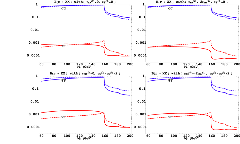
Figure 3: In these plots, we show the branching fractions of the radion into gluons and photons (the solid lines), comparing with RS1 scenario (the dashed curves). For each graph, the solid curves represent the branching fractions in the presence of different combinations of tree level brane localized kinetic terms for the gluon and photon. The magnitudes of the localized terms are given on the top of every plot individually in units of the one-loop corrections to the $\tau^{\rm UV}_{i}$. We have set $\Lambda_{r}=2$ TeV, corresponding to $1/R^{\prime}=816$ GeV.

Note that in the absence of sizable tree level brane localized kinetic terms, the branching fractions for the massless gauge bosons are slightly larger in comparison with the RS1 case. The effect of introducing significant tree level brane localized kinetic terms is to reduce the branching fractions for the corresponding gauge boson. This is due to the fact that the effect of positive BKTs cancels against the term that scales as $1/\log R^{\prime}/R$. In the presence of a tree level brane localized kinetic term for the gluon only, the branching fraction to photons is enhanced. The reason for this is that the decay to gluons is the dominant mode. Once a BKT for the gluon is added, the partial width to gluons decreases, thereby increasing the branching fractions to subdominant channels.

In Figure 4, we demonstrate how the branching fractions of the radion into all SM particles change in the presence of tree level brane localized gauge boson kinetic terms. The branching fractions to massive gauge bosons, Higgs bosons, and top quarks are not significantly different compared to the original RS1 scenario. Note however that the branching fraction to gluons (and thus the production rate) for larger radion masses still differs from the values found in the brane localized SM.

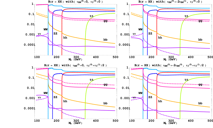
Figure 4: In this plot, we show the branching fractions of the radion into on-shell final states. Again, the dashed curves represent the branching fractions in the RS1 scenario. We show the effect of introducing tree level brane localized kinetic terms for the photon and gluon, choosing different combinations for each graph. We set $\Lambda_{r}=2$ TeV, corresponding to an IR brane scale of $1/R^{\prime}=816$ GeV.

7 Discovery potential at the LHC

In this section we discuss the radion discovery potential at the LHC. We show plots of the ratio of the discovery significance of the radion in the $gg\rightarrow r\rightarrow ZZ\rightarrow 4l$ and $gg\rightarrow r\rightarrow\gamma\gamma$ channels and those of a SM Higgs boson with the same mass. An approximate formula for the ratio of the significance of potential radion discovery compared with a SM Higgs boson discovery of the same mass for the $gg\rightarrow r\rightarrow\gamma\gamma$ channel is given in [4]:

$$R_{S}^{\gamma\gamma}\equiv\frac{S(r)}{S(h_{SM})}=\frac{\Gamma(r\rightarrow gg)\,B(r\rightarrow\gamma\gamma))}{\Gamma(h_{SM}\rightarrow gg)\,B(h_{SM}\rightarrow\gamma\gamma))}\sqrt{\frac{max(\Gamma_{tot}(h_{SM}),\Delta M_{\gamma\gamma})}{max(\Gamma_{tot}(r),\Delta M_{\gamma\gamma})}},$$ (7.1)

with a similar formula applying for the significance ratio in the $r\rightarrow ZZ$ discovery channel.

The factor inside the square root measures the ratio of the relative effective total widths of the Higgs and radion as they would appear in the detector. For smaller widths, the signal to background ratio is higher, although this effect is limited by the detector resolution for diphoton (or 4 lepton) invariant masses. If the total width is smaller than the energy resolution, the entire signal is contained in a single bin, and one then needs to consider the background over that entire region (rather than only over the energy range given by the width of the decaying particle).

Figure 5: In the plot on the left,we show a comparison of the ratio of discovery significance for a radion vs. a Higgs of the same mass, $R^{\gamma\gamma}_{S}$, with the scenario where the SM fields are all localized on the IR brane (the dashed curves). In the plot on the right we show the ratio of discovery significance $R^{4l}_{S}$. We assume that there are no tree level brane localized kinetic terms for the gluon or photon. For the displayed values of $\Lambda_{r}$, the corresponding values of $1/R^{\prime}$ are $408$, $816$, $2041$, and $4082$ GeV.

In Fig. 5 we plot $R^{\gamma\gamma}_{S}$ and $R^{4l}_{S}$ in the case that there are no tree level brane localized kinetic terms for either the gluon or photon. We find that for low values of $\Lambda_{r}$, the ratio $R^{\gamma\gamma}_{S}$ is always greater than one, implying that one is more likely to find a radion of this mass than a Higgs of the same mass. For some values of the radion mass, $R^{\gamma\gamma}_{S}$, is enhanced compared to the case with all fields localized on the IR brane, up to a factor of 3 for large values of $\Lambda_{r}$. In the $r\rightarrow 4l$ channel, there is a generic enhancement of the discovery potential in comparison with the IR brane localized SM scenario due to the larger $r\rightarrow gg$ branching fraction.

In Fig. 6 we plot $R^{\gamma\gamma}_{S}$ for different combinations of tree level brane localized kinetic terms for both the gluon and the photon, taking $\Lambda_{r}=2$ TeV. One can see that turning on positive BKTs generically reduces the potential radion signal in the diphoton channel, and that the signal can even be reduced compared to the traditional RS1 model.

Figure 6: In this figure, we show the ratio of the discovery significance $R^{\gamma\gamma}_{S}$ with $\Lambda_{r}=2$ TeV for various combinations of tree level brane localized kinetic terms for the photon and gluon. We have set $\Lambda_{r}=2$ TeV, corresponding to an IR brane with $1/R^{\prime}=816$ GeV. Again, the dashed curves represent the signal significance in the original RS1 model.

Finally, in Fig. 7 we plot $R^{\gamma\gamma}_{S}$ and $R^{4l}_{S}$ for different values of the tree level brane localized kinetic term for the gluon, taking $\Lambda_{r}=2$ TeV, and $\tau_{EM}^{(0)}=0$. The signal significance $R^{4l}_{S}$ is insensitive to brane localized kinetic terms for the photon. We choose three values for the gluon UV BKT, $\tau_{3}^{(0)}=0$, $\tau_{3}^{(1)}/2$, and $\tau_{3}^{(1)}$. The first two are well within the perturbativity constraint in Eq. (6.2), while the last choice saturates it. For the last case, the branching fraction to gluons is quite suppressed, as the large QCD conformal anomaly contribution is nearly canceled by the gluon BKT. The production cross section is therefore strongly quenched. We find in this last case that the signal significance can be significantly smaller (by a factor of 10) compared to the traditional RS1 model.

Figure 7: In this figure, we compare the discovery significance in $\gamma\gamma$ and $4l$ in the presence of a UV brane localized kinetic term for the gluon only: $\tau_{EM}^{(0)}=0$. The curves that are (dashed, solid, dashed-dotted, dotted) correspond to the RS1 scenario, $\tau_{3}^{(0)}=0$, $\tau_{3}^{(0)}=\tau_{3}^{(1)}/2$, and $\tau_{3}^{(0)}=\tau_{3}^{(1)}$, respectively. This last value saturates the perturbativity bound in Eq. (6.2) for most values of $\Lambda_{IR}$.

For all cases we have considered, there is a small region where $R^{\gamma\gamma}_{S}$ is sharply suppressed, corresponding to the $\sim 160$ GeV threshold at which the radion decay to $WW$ turns on, and the normalized signal significance of $gg\rightarrow r\rightarrow\gamma\gamma$ drops sharply. In addition, there is a sharp step when $R^{4l}_{S}$ becomes well defined (when the on-shell decays $r,h\rightarrow ZZ$ are kinematically allowed). We note that this behavior is softened if one takes into account decay channels which pass through off-shell $W$ or $Z$ bosons, and that the gap between the $WW$ and $ZZ$ thresholds is in fact covered by the $4l$ signal with an off-shell intermediate $Z$-boson.

In summary, we have found that there are large regions of parameter space where one is as likely to find a radion as a SM Higgs of the same mass. With $100$ fb^-1 of data, it is projected that a SM Higgs would be discovered with a confidence level of between $10$ and $13$ sigma for Higgs masses between $100$ and $1000$ GeV. Therefore if the solution of the SM hierarchy problem involves warped extra dimensions, it is not unlikely that we will discover a radion at the LHC. When we find a new particle with Higgs-like signatures, it becomes a matter of deciding whether or not we have found “The Higgs.” In the large mass region (when the resonance is above about $230$ GeV), a SM Higgs boson would have a width which is resolvable by the detector, while the radion width is much narrower. A width measurement could exclude a conventional SM Higgs boson as a candidate for this new state. The smaller mass range deserves further study, as a width measurement will not suffice, making discrimination more difficult. Precision measurements (such as those that would be performed at a linear collider), coupled with a discovery of KK towers for the SM gauge and matter fields would provide further evidence helping to confirm the discovery of a RS radion.

8 Conclusions

We have investigated the phenomenology of the RS radion in models where the SM fields propagate in the bulk as opposed to being confined to the IR brane in the traditional RS1 model. The motivation for this is that most realistic models of EWSB utilize such a setup. We have calculated the radion couplings to the SM fields in detail, and we have given a CFT interpretation for all of these interactions. We have paid special attention to the couplings to massless gauge bosons, since these are phenomenologically the most important ones, and since the one-loop effects are significant. We then compared the radion discovery potential of the LHC to that for a SM Higgs, and also to the radion of the traditional RS1 model. We have found that the $\gamma\gamma$ signal is enhanced over the SM Higgs case for some reasonable values of the RS scale. However, this signal depends quite sensitively on the values of the brane localized kinetic terms for the massless gauge fields. If those are sizeable, the significance of the signal can decrease, becoming smaller than in the traditional RS1 case. Finally, we have shown that for the region of larger radion masses where the $\gamma\gamma$ signal is no longer significant, one can use the 4 lepton signal to look for the radion. If a new Higgs-like state is discovered at the LHC, a width measurement could rule out a conventional Higgs boson, however further discoveries involving KK modes and precision studies of the scalar sector would be necessary to provide convincing evidence for a RS radion.

Appendix

A The cancellation of the boundary couplings with fermions

The actual construction for fermion masses for the bulk fermions involves adding boundary mass terms for the fermions of the form

$$-\int d^{4}x\sqrt{g^{ind}}M_{D}R^{\prime}(\psi_{R}\chi_{L}+h.c.)$$ (A.1)

Note, that since $\psi,\chi$ are bulk fermions, the actual mass parameter is a dimensionless ${\cal O}(1)$ coupling which we denote for convenience denote by $M_{D}R^{\prime}$. Expanding this in terms of the radion field we obtain the boundary coupling

$$\int d^{4}x\left(\frac{R}{R^{\prime}}\right)^{4}4FM_{D}R^{\prime}(\psi_{R}\chi_{L}+h.c.).$$ (A.2)

However, there is an additional localized coupling term from the discontinuity of the fermion wave functions around the TeV brane. The simplest way to see the emergence of this term is by assuming that the actual BC’s at the TeV brane are $\chi_{R}=\psi_{L}=0$ irrespectively of the boundary mass term, and then add the boundary mass a distance $\epsilon$ away from the TeV brane. The effect of this boundary mass (A.1) will then be to induce a discontinuity in the fermion wave functions

$$[\chi_{R}]\equiv-\chi_{R}|_{R^{\prime}-\epsilon}+\chi_{R}|_{R^{\prime}},\ \ [\psi_{L}]\equiv-\psi_{L}|_{R^{\prime}-\epsilon}+\psi_{L}|_{R^{\prime}}.$$ (A.3)

Here $\chi_{R}|_{R^{\prime}}$ and $\psi_{L}|_{R^{\prime}}$ are still fixed to zero, and the limiting values at distance $\epsilon$ are the fields appearing in the boundary conditions for the fermions. Then the bulk action will also give a contribution to the radion coupling with magnitude

$$\int d^{4}x\left(\frac{R}{R^{\prime}}\right)^{4}2F(\psi_{R}[\chi_{R}]-[\psi_{L}]\chi_{L}+h.c.).$$ (A.4)

However, evaluating the discontinuities using the fermion BC’s we find that (A.4) exactly cancels (A.2).

B Fermion masses from CFT

We have seen from the explicit calculation that the approximate expression for the fermion masses is given by (3.11). Here we present a simple derivation of this result from the CFT point of view. Most of the elements of this are already implicitly contained in [11]. As explained in Section 5, the fermion zero mode (before EWSB) is interpreted as a mixture of an elementary fermion $\chi_{L}$ with an with a composite operator ${\cal O}_{L}$ (and similarly the right handed $\psi_{R}$ is mixed with ${\cal O}_{R}$). The mixing among these fields is determined by the wave function of the actual zero mode on the IR brane:

$$\omega_{R,L}=\sqrt{\frac{1\pm 2c_{R,L}}{1-(\frac{R}{R^{\prime}})^{1\pm 2c_{R,L}}}}$$ (B.1)

Thus the mixture that is the zero mode can be identified with (assuming $\omega_{L,R}\ll 1$)

$$\chi_{light}=\chi_{L}-\omega_{L}{\cal O}_{L}\ ,\ \psi_{light}=\psi_{R}-\omega_{R}{\cal O}_{R}\ .$$ (B.2)

As discussed in Sec. 5 the electroweak symmetry breaking mass term is given by $M_{D}{\cal O}_{L}{\cal O}_{R}$. Expressing ${\cal O}_{L,R}$ in terms of the light fields we find that the mass for the light fields is given by

$$M^{2}=M_{D}^{2}\omega_{L}^{2}\omega_{R}^{2}=M_{D}^{2}\frac{(1-2c_{L})(1+2c_{R})}{(1-(\frac{R}{R^{\prime}})^{1-2c_{L}})(1-(\frac{R}{R^{\prime}})^{1+2c_{R}})}.$$ (B.3)

This agrees with the expression (3.11). For $c_{L}>1/2,c_{R}<-1/2$ this simplifies to

$$\frac{\lambda}{R}\sqrt{(2c_{L}-1)(-1-2c_{R})}\left(\frac{R^{\prime}}{R}\right)^{c_{R}-c_{L}},$$ (B.4)

where $\lambda=M_{D}R^{\prime}$ is the fundamental parameter that we are adding to the theory. One can read off the radion coupling from this form of the mass formula by substituting the $R^{\prime}$ dependence with the radion.

C Cancellation of linear divergences

In the 5D theory, there are potential linear divergences in the coupling of the radion to the gauge boson zero modes. In this appendix, we show that the linear divergences in fact cancel once the theory is renormalized.

For the purposes of this demonstration, we work with a simpler theory, a bulk scalar version of QED. The action is given by

$$S=\int d^{5}x-\frac{1}{4}(1+\delta_{A}(z))F_{MN}^{2}+|D_{M}\phi|^{2}-M^{2}|\phi|^{2},$$ (C.1)

where we have included the counterterm for divergences in the 5D field strength one-loop effective action.

The bulk operator which determines the radion coupling to the bulk scalar field is given by

$$3T_{55}g^{55}-\mathrm{Tr~{}}T_{MN}=-6\left(\frac{z}{R}\right)^{2}|\nabla_{5}\phi|^{2}+(d-4)|D_{R}\phi|^{2},$$ (C.2)

where we have set $\mathrm{Tr~{}}g_{\mu\nu}=d$ to work in dimensional regularization.

The radion couples to the gauge fields directly through the counterterm necessary to cancel the one-loop divergence in the gauge boson self energy:

$$3T_{55}g^{55}-\mathrm{Tr~{}}T_{MN}=(1+\delta_{A}(z))\left(\frac{6-d}{2}\right)\left(\frac{z}{R}\right)^{4}A_{\mu}\left(-g^{\mu\nu}q^{2}+q^{\mu}q^{\nu}\right)A_{\nu}$$ (C.3)

At one loop, there are two contributions to the radion coupling. These are the direct coupling to the counterterm above, and the triangle diagram involving a coupling of the radion to the bulk scalar.

The counterterm is due to the self energy diagram, which is given by

$$\frac{1}{2}g_{5}^{2}\int\frac{d^{d}p}{(2\pi)^{d}}(2p+q)^{\mu}(2p+q)^{\nu}\int_{R}^{R^{\prime}}dzdv\left(\frac{R}{z}\right)^{3}\left(\frac{R}{v}\right)^{3}G_{|p|}(z,v)G_{|p+q|}(v,z).$$ (C.4)

To study the most divergent contribution to the self energy diagram, we consider the high momentum limit of the full 5D propagator:

$$G_{p}(z,z^{\prime})\approx\left(\frac{zz^{\prime}}{R^{2}}\right)^{3/2}\frac{\cosh{(p(z-R))}\cosh{(p(R^{\prime}-z^{\prime}))}}{p\sinh{(p(R^{\prime}-R))}}.$$ (C.5)

Performing the integral over $v$, and considering only the leading term in the $1/|p|$ expansion, Equation (C.4) reduces to

$$\frac{1}{2}g_{5}^{2}\int\frac{d^{d}p}{(2\pi)^{d}}(2p+q)^{\mu}(2p+q)^{\nu}\int_{R}^{R^{\prime}}dz\frac{1}{2|p|(|p|+|q|)(2|p|+|q|)}.$$ (C.6)

We then expand Eq. (C.6) about small external momentum $q$, and consider only the terms which are second order in $q$. The lower order terms in the expansion lead to cubic divergences which vanish due to the 5D Ward identity.

After this expansion, and utilizing the symmetries of the momentum integrals, the self energy diagram becomes

$$\frac{1}{24}g_{5}^{2}\left[-g^{\mu\nu}q^{2}\left(\frac{9}{d}-\frac{30}{d(d+2)}\right)+q^{\mu}q^{\nu}\left(3-\frac{18}{d}+\frac{60}{d(d+2)}\right)\right]\int_{R}^{R^{\prime}}dz\int\frac{d^{d}p}{(2\pi)^{d}}\frac{1}{|p|^{3}}$$

$$\equiv\frac{1}{24}g_{5}^{2}P^{\mu\nu}_{\rm SE}(d)\int_{R}^{R^{\prime}}dz\int\frac{d^{d}p}{(2\pi)^{d}}\frac{1}{|p|^{3}},$$ (C.7)

where $P^{\mu\nu}_{\rm SE}=(-g^{\mu\nu}q^{2}+q^{\mu}q^{\nu})$ both when $d=3$ and $d=4$. The counterterm contribution to the radion operator is then given by

$$-\frac{6-d}{24}\left(\frac{z}{R}\right)^{5}g_{5}^{2}A_{\mu}P^{\mu\nu}_{\rm SE}(d)A_{\nu}\int\frac{d^{d}p}{(2\pi)^{d}}\frac{1}{|p|^{3}}.$$ (C.8)

We now turn our attention to the triangle diagram where the radion couples to gauge bosons through a scalar loop. The one loop matrix element of the scalar contribution to the radion operator between two gauge fields is given by

$$6g_{5}^{2}\left(\frac{z}{R}\right)^{2}\int\frac{d^{d}p}{(2\pi)^{d}}(2p+q)^{\mu}(2p+q)^{\nu}\int_{R}^{R^{\prime}}dwdv\left(\frac{R}{v}\right)^{3}\left(\frac{R}{w}\right)^{3}\partial_{z}G_{|p|}(v,z)\partial_{z}G_{|p|}(z,w)G_{|p+q|}(v,w).$$ (C.9)

Note that the last term in Eq. (C.2) does not contribute after imposing the equation of motion for $\phi$.

Performing the integrals along the extra dimension, and expanding in small external momentum $q$, Eq. (C.9) becomes

$$\frac{1}{8}g_{5}^{2}\left(\frac{z}{R}\right)^{5}\left[-g^{\mu\nu}q^{2}\left(\frac{6}{d}-\frac{15}{d(d+2)}\right)+q^{\mu}q^{\nu}\left(3-\frac{12}{d}+\frac{30}{d(d+2)}\right)\right]\int\frac{d^{d}p}{(2\pi)^{d}}\frac{1}{|p|^{3}}.$$ (C.10)

Thus the triangle diagram contributes the following to the radion operator at one loop:

$$\frac{1}{8}g_{5}^{2}\left(\frac{z}{R}\right)^{5}A_{\mu}P^{\mu\nu}_{\bigtriangleup}(d)A_{\nu}\int\frac{d^{d}p}{(2\pi)^{d}}\frac{1}{|p|^{3}},$$ (C.11)

where $P^{\mu\nu}_{\bigtriangleup}=(-g^{\mu\nu}q^{2}+q^{\mu}q^{\nu})$ both when $d=1$ and $d=3$.

Summing up the two contributions, we find

$$\frac{1}{8}g_{5}^{2}\left(\frac{z}{R}\right)^{5}A_{\mu}\left[P^{\mu\nu}_{\bigtriangleup}(d)-\frac{6-d}{3}P^{\mu\nu}_{\rm SE}\right]\int\frac{d^{d}p}{(2\pi)^{d}}\frac{1}{|p|^{3}}$$

$$=-\frac{1}{4}g_{5}^{2}\left(\frac{z}{R}\right)^{5}A_{\mu}\left[-g^{\mu\nu}\frac{3d-7}{d(d+2)}+q^{\mu}q^{\nu}\frac{d^{2}-4d+14}{d(d+2)}\right]\left(\frac{3}{2}-\frac{d}{2}\right)\int\frac{d^{d}p}{(2\pi)^{d}}\frac{1}{|p|^{3}}$$

(C.12)

The momentum integral is proportional to $\Gamma(3/2-d/2)$, signalling a linear divergence, however, the coefficient is proportional to $(3/2-d/2)$. Combining this with the $\Gamma$-function gives a result which is convergent even as $d\rightarrow 4$. Thus this contribution is in fact finite. Note however that this expression is not transverse as $d\rightarrow 4$. This is because an expansion to higher order in the external momentum $q$ is necessary to capture the complete finite contribution.

References

- [1] L. Randall and R. Sundrum, Phys. Rev. Lett. 83, 3370 (1999) [arXiv:hep-ph/9905221].
- [2] W. D. Goldberger and M. B. Wise, Phys. Rev. Lett. 83, 4922 (1999) [arXiv:hep-ph/9907447]; Phys. Lett. B 475, 275 (2000) [arXiv:hep-ph/9911457].
- [3] C. Csáki, M. Graesser, L. Randall and J. Terning, Phys. Rev. D 62, 045015 (2000) [arXiv:hep-ph/9911406].
- [4] G. F. Giudice, R. Rattazzi and J. D. Wells, Nucl. Phys. B 595, 250 (2001) [arXiv:hep-ph/0002178].
- [5] T. Tanaka and X. Montes, Nucl. Phys. B 582, 259 (2000) [arXiv:hep-th/0001092].
- [6] C. Csáki, M. L. Graesser and G. D. Kribs, Phys. Rev. D 63, 065002 (2001) [arXiv:hep-th/0008151].
- [7] D. Dominici, B. Grzadkowski, J. F. Gunion and M. Toharia, Nucl. Phys. B 671, 243 (2003) [arXiv:hep-ph/0206192]; J. F. Gunion, M. Toharia and J. D. Wells, Phys. Lett. B 585, 295 (2004) [arXiv:hep-ph/0311219].
- [8] S. Bae, P. Ko, H. S. Lee and J. Lee, arXiv:hep-ph/0103187.
- [9] N. Arkani-Hamed, M. Porrati and L. Randall, JHEP 0108, 017 (2001) [arXiv:hep-th/0012148]; R. Rattazzi and A. Zaffaroni, JHEP 0104, 021 (2001) [arXiv:hep-th/0012248].
- [10] K. Agashe and A. Delgado, Phys. Rev. D 67, 046003 (2003) [arXiv:hep-th/0209212].
- [11] R. Contino and A. Pomarol, JHEP 0411, 058 (2004) [arXiv:hep-th/0406257].
- [12] H. Davoudiasl, J. L. Hewett and T. G. Rizzo, Phys. Lett. B 473, 43 (2000) [arXiv:hep-ph/9911262]; A. Pomarol, Phys. Lett. B 486, 153 (2000) [arXiv:hep-ph/9911294].
- [13] C. Csáki, J. Erlich and J. Terning, Phys. Rev. D 66, 064021 (2002) [arXiv:hep-ph/0203034]; J. L. Hewett, F. J. Petriello and T. G. Rizzo, JHEP 0209, 030 (2002) [arXiv:hep-ph/0203091].
- [14] K. Agashe, A. Delgado, M. J. May and R. Sundrum, JHEP 0308, 050 (2003) [arXiv:hep-ph/0308036].
- [15] C. Csáki, C. Grojean, L. Pilo and J. Terning, Phys. Rev. Lett. 92, 101802 (2004) [arXiv:hep-ph/0308038].
- [16] R. Contino, Y. Nomura and A. Pomarol, Nucl. Phys. B 671, 148 (2003) [arXiv:hep-ph/0306259]; K. Agashe, R. Contino and A. Pomarol, Nucl. Phys. B 719, 165 (2005) [arXiv:hep-ph/0412089].
- [17] T. G. Rizzo, JHEP 0206, 056 (2002) [arXiv:hep-ph/0205242].
- [18] C. Csáki, C. Grojean, J. Hubisz, Y. Shirman and J. Terning, Phys. Rev. D 70, 015012 (2004) [arXiv:hep-ph/0310355].
- [19] Y. Grossman and M. Neubert, Phys. Lett. B 474, 361 (2000) [arXiv:hep-ph/9912408].
- [20] T. Gherghetta and A. Pomarol, Nucl. Phys. B 586, 141 (2000) [arXiv:hep-ph/0003129].
- [21] S. J. Huber and Q. Shafi, Phys. Lett. B 498, 256 (2001) [arXiv:hep-ph/0010195].
- [22] L. Randall and M. D. Schwartz, JHEP 0111, 003 (2001) [arXiv:hep-th/0108114].
- [23] W. D. Goldberger and I. Z. Rothstein, Phys. Rev. Lett. 89, 131601 (2002) [arXiv:hep-th/0204160]; Phys. Rev. D 68, 125011 (2003) [arXiv:hep-th/0208060]; Phys. Rev. D 68, 125012 (2003) [arXiv:hep-ph/0303158].
- [24] K. w. Choi and I. W. Kim, Phys. Rev. D 67, 045005 (2003) [arXiv:hep-th/0208071].
- [25] K. Agashe, A. Delgado and R. Sundrum, Nucl. Phys. B 643, 172 (2002) [arXiv:hep-ph/0206099]; Annals Phys. 304, 145 (2003) [arXiv:hep-ph/0212028].
- [26] R. Contino, P. Creminelli and E. Trincherini, JHEP 0210, 029 (2002) [arXiv:hep-th/0208002].