Orbital magnetization and Chern number in a supercell framework:
Single k-point formula

Abstract

The key formula for computing the orbital magnetization of a crystalline system has been recently found [D. Ceresoli, T. Thonhauser, D. Vanderbilt, R. Resta, Phys. Rev. B 74, 024408 (2006)]: it is given in terms of a Brillouin-zone integral, which is discretized on a reciprocal-space mesh for numerical implementation. We find here the single ${\bf k}$-point limit, useful for large enough supercells, and particularly in the framework of Car-Parrinello simulations for noncrystalline systems. We validate our formula on the test case of a crystalline system, where the supercell is chosen as a large multiple of the elementary cell. We also show that—somewhat counterintuitively—even the Chern number (in 2d) can be evaluated using a single Hamiltonian diagonalization.

The position operator ${\bf r}$ is ill-defined within periodic boundary conditions. Owing to this, both the macroscopic (electrical) polarization and the macroscopic orbital magnetization are nontrivial quantities in condensed-matter theory. The former has been successfully tamed since the early 1990s, when the modern theory of polarization, based on a Berry phase, was developed.KSV ; rap_a12 The latter, instead, remained an unsolved problem until 2005. Since then, several important papers have appearedrap126 ; Xiao05 ; rap128 ; rap130 ; Xiao07 and continue to appear.Shi07 Before 2005 only linear-response properties related to orbital magnetization were successfully addressed,linear ; Mauri while we stress that the present work, as well as Refs. rap126, ; Xiao05, ; rap128, ; rap130, ; Xiao07, ; Shi07, , addresses “magnetization itself”.

A general formula, valid for crystalline systems within a given single-particle Hamiltonian, was provided in Ref. rap130, , hereafter referred to as I. This is the magnetic analogue of the (by now famous) King-Smith and Vanderbilt formula for electrical polarization.KSV Both formulas are discretized on a regular mesh of ${\bf k}$ points for numerical implementation. However, most simulations for noncrystalline systems, particularly those of the Car-Parrinello type,CP are routinely performed by diagonalizing the Hamiltonian at a single ${\bf k}$ point (the $\Gamma$ point) in a large supercell. The reduction from many points to a single point is far from being trivial; nonetheless a successful single-point formula for electrical polarization emerged since 1996, and is universally used since then.trois ; rap100 We provide here the magnetic analogue of such formula. As a byproduct, one can even evaluate the Chern number Thouless using a single ${\bf k}$ point. This looks like an oxymoron, given that the Chern number is by definition a loop integral in reciprocal space: but our formula can be regarded as the limiting case where the loop shrinks to a single point.

The general formula of I applies to normal periodic insulators (where the Chern invariant vanishes), Chern insulators (where the Chern invariant is nonzero), and metals. Aiming at first-principle implementations within any flavor of DFT, the single-particle Hamiltonian is the Kohn-Sham one.DFT As for the analogous case of electrical polarization, there is no guarantee that the Kohn-Sham magnetization coincides with the actual one. Nonetheless, previous studies within linear-response methods indicate that even for orbital magnetization the error is small.Mauri

As in I, we assume a vanishing macroscopic magnetic field ${\bf B}$, hence a lattice-periodical Hamiltonian. We let $\epsilon_{n{\bf k}}$ and $|\psi_{n{\bf k}}\rangle$ be the Bloch eigenvalues and eigenvectors of $H$, respectively, and $u_{n{\bf k}}({\bf r})={\rm e}^{-i{\bf k}\cdot{\bf r}}\psi_{n{\bf k}}({\bf r})$ be the corresponding eigenfunctions of the effective Hamiltonian

$$H_{\bf k}={\rm e}^{-i{\bf k}\cdot{\bf r}}H{\rm e}^{i{\bf k}\cdot{\bf r}}\,;$$ (1)

we normalize them to one over the crystal cell of volume $V$. As in I, the notation is intended to be flexible as regards the spin character of the electrons. If we deal with spinless electrons, then $n$ is a simple index labeling the occupied Bloch states; factors of two may trivially be inserted if one has in mind degenerate, independent spin channels. For the sake of simplicity, we rule out the metallic case here. For both normal insulators and Chern insulators the macroscopic orbital magnetization ${\bf M}$ is, according to I:

$$M_{\gamma} = -\frac{\varepsilon_{\gamma\alpha\beta}}{2c(2\pi)^{3}}$$

$$\times {\rm Im}\,\sum_{n}\int\!d{\bf k}\;\langle\partial_{\alpha}u_{n{\bf k}}|(\,H_{\bf k}+\epsilon_{n{\bf k}}-2\mu\,)\,|\partial_{\beta}u_{n{\bf k}}\rangle\;,$$

where Greek subscripts are Cartesian indices, $\varepsilon_{\gamma\alpha\beta}$ is the antisymmetric tensor, $\partial_{\alpha}=\partial/\partial k_{\alpha}$, $\mu$ is the chemical potential (Fermi energy), the integration is over the reciprocal cell, and the sum over Cartesian indices is implied. For insulators the number of states with energy $\epsilon_{n{\bf k}}\leq\mu$ is independent of ${\bf k}$; we implicitly understand the sum in Eq. (Orbital magnetization and Chern number in a supercell framework: Single k-point formula) as on these states only.

As usual, a noncrystalline system can be dealt with in a supercell framework, by addressing an artificial crystal with a large unit cell, actually larger than the relevant correlation length. One key feature of Eq. (Orbital magnetization and Chern number in a supercell framework: Single k-point formula) is its gauge-invariance in the generalized sense: by this we mean that Eq. (Orbital magnetization and Chern number in a supercell framework: Single k-point formula) is invariant by unitary mixing of the occupied states among themselves at a any given ${\bf k}$. Thanks to such key feature Eq. (Orbital magnetization and Chern number in a supercell framework: Single k-point formula) is invariant by cell doubling. In fact, starting with a cell (or supercell) of given size, we may regard the same physical system as having double periodicity (in all directions), in which case the integration domain in Eq. (Orbital magnetization and Chern number in a supercell framework: Single k-point formula) gets “folded” and shrinks by a factor $1/8$, while the number of occupied eigenstates gets multiplied by a factor of $8$. It is easy to realize that these are in fact the same eigenstates as in the unfolded case, apart possibly for a unitary transformation, irrelevant here. As for actual computations, the discretized form of Eq. (Orbital magnetization and Chern number in a supercell framework: Single k-point formula) adopted in I turns to be invariant by cell doubling to within $10^{-5}$, provided the ${\bf k}$-point mesh is chosen consistently.

For a large supercell of volume $V$ the integration domain in Eq. (Orbital magnetization and Chern number in a supercell framework: Single k-point formula) becomes small. Therefore the integral can be accurately approximated by the value of the integrand at ${\bf k}=0$, times the reciprocal-cell volume:

$$M_{\gamma}\simeq-\frac{\varepsilon_{\gamma\alpha\beta}}{2cV}\,\,{\rm Im}\,\sum_{n}\langle\partial_{\alpha}u_{n0}|(\,H_{0}+\epsilon_{n0}-2\mu\,)\,|\partial_{\beta}u_{n0}\rangle\;.$$ (3)

Notice that Eq. (Orbital magnetization and Chern number in a supercell framework: Single k-point formula) can be safely approximated with Eq. (3) because the integrand is a gauge-invariant quantity; the apparently analogous case of polarization is more difficult, since the integrand therein is gauge-dependent, and the single-point formula requires a less straightforward treatment.trois ; rap100 As for the derivatives in Eq. (3), they can be evaluted in two ways: either “analytically” (by means of perturbation theory), or “numerically” (by means of finite differences).

The analytical-derivative approach relies on the perturbation formula

$$|\partial_{\alpha}u_{n0}\rangle=\sum_{m\neq n}|u_{m0}\rangle\frac{\langle u_{m0}|v_{\alpha}|u_{n0}\rangle}{\epsilon_{m0}-\epsilon_{n0}}\;,$$ (4)

where $v_{\alpha}$ is the $\alpha$-component of the velocity operator

$${\bf v}=i[H,{\bf r}]=\left.\nabla_{\bf k}H_{\bf k}\right|_{{\bf k}=0}\;.$$ (5)

Eq. (4) is convenient for tight-binding implementations, where the sum is over a small number of terms. We also notice that the matrix representation of ${\bf r}$, for use in Eqs. (1) and (5), is usually taken to be diagonal on the tight-binding basis.

The numerical-derivative approach looks more convenient for first-principle implementations, since it requires neither the (slowly convergent) sum over states, nor the matrix elements of the velocity operator. In order to give the most general formulation for non-rectangular cells it is expedient to switch to a coordinate-independent form. In order to shorten the equations, in all of the following developments of Eq. (3) a sum over the occupied states is implied.

If ${\bf b}_{j}$ are the shortest reciprocal vectors of the supercell, Eq. (3) can be identically recast as

$${\bf M}\simeq-\frac{\varepsilon_{ijl}{\bf b}_{i}|{\bf b}_{j}||{\bf b}_{l}|}{2c(2\pi)^{3}}\,{\rm Im}\,\langle\partial_{j}u_{n0}|(\,H_{0}+\epsilon_{n0}-2\mu\,)\,|\partial_{l}u_{n0}\rangle.$$ (6)

where a sum over $ijl$ is implied, and $\partial_{j}$ indicates the partial derivative in the direction of ${\bf b}_{j}$:

$$|\partial_{j}u_{n0}\rangle=\lim_{\lambda\rightarrow 0}\;\frac{1}{\lambda|{\bf b}_{j}|}(\,|u_{n\,\lambda{\bf b}_{j}}\rangle-|u_{n0}\rangle\,).$$ (7)

Notice that Eq. (7) implicitly assumes that $|u_{n{\bf k}}\rangle$ is a differentiable function: but this is generally not the case when the eigenstates are obtained from numerical diagonalization. The discretization must then be done in a specific gauge: as in I, we fix the problem by adopting the “covariant derivative” approach, introduced in Refs. Sai02, and Souza04, . One defines the overlap matrix $S_{nn^{\prime}}({\bf k})=\langle u_{n0}|u_{n^{\prime}{\bf k}}\rangle$, and the “dual” states

$$|\tilde{u}_{n{\bf k}}\rangle=\sum_{n^{\prime}}S^{-1}_{n^{\prime}n}({\bf k})\,|u_{n^{\prime}{\bf k}}\rangle,$$ (8)

which enjoy the property $\langle u_{n0}|\tilde{u}_{n^{\prime}{\bf k}}\rangle=\delta_{nn^{\prime}}$. Using this, approximating Eq. (7) with its $\lambda=1$ value, and inserting in Eq. (6) we finally get

$${\bf M}\simeq-\frac{\varepsilon_{ijl}{\bf b}_{i}}{2c(2\pi)^{3}}\,{\rm Im}\,\langle\tilde{u}_{n{\bf b}_{j}}|(\,H_{0}+\epsilon_{n0}-2\mu\,)\,|\tilde{u}_{n{\bf b}_{l}}\rangle.$$ (9)

Next, we wish to evaluate $|\tilde{u}_{n{\bf b}_{j}}\rangle$ without actually diagonalizing the Hamiltonian at ${\bf k}\neq 0$. To this aim, we notice that the state ${\rm e}^{-i{\bf b}_{j}\cdot{\bf r}}|u_{n0}\rangle$ obeys periodic boundary conditions and is an eigenstate of $H_{n{\bf b}_{j}}$ corresponding, possibly, to a different occupied eigenvalue. The transformation in Eq. (8) restores the correct ordering anyhow; therefore we can simply identify $|u_{n{\bf b}_{j}}\rangle={\rm e}^{-i{\bf b}_{j}\cdot{\bf r}}|u_{n0}\rangle$, transform to the dual states by means of Eq. (8), and insert into Eq. (9) which eventually becomes the single-point, ${\bf k}=0$ formula, aimed at.

For a two-dimensional (2d) system the magnetization is a pseudoscalar, and the analogue of Eq. (9) reads

$$M=-\frac{|{\bf b}_{1}\times{\bf b}_{2}|}{c(2\pi)^{2}|{\bf b}_{1}|\,|{\bf b}_{2}|}\,{\rm Im}\,\langle\tilde{u}_{n{\bf b}_{1}}|(\,H_{0}+\epsilon_{n0}-2\mu\,)\,|\tilde{u}_{n{\bf b}_{2}}\rangle.$$ (10)

Similarly, the single-point formula for the Chern number reads

$$C=-\frac{|{\bf b}_{1}\times{\bf b}_{2}|}{2\pi|{\bf b}_{1}|\,|{\bf b}_{2}|}\,{\rm Im}\,\langle\tilde{u}_{n{\bf b}_{1}}|\tilde{u}_{n{\bf b}_{2}}\rangle.$$ (11)

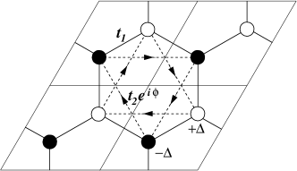
Figure 1: Four unit cells of the Haldane model. Filled (open) circles denote sites with $E_{0}=-\Delta$ ($+\Delta$). Solid lines connecting nearest neighbors indicate a real hopping amplitude $t_{1}$; dashed arrows pointing to a second-neighbor site indicates a complex hopping amplitude $t_{2}e^{i\phi}$. Arrows indicate sign of the phase $\phi$ for second-neighbor hopping.

As in previous works, rap128 ; rap130 we find expedient to validate the present findings on the Haldane model Hamiltonian:Haldane88 it is comprised of a 2d honeycomb lattice with two tight-binding sites per primitive cell with site energies $\pm\Delta$, real first-neighbor hoppings $t_{1}$, and complex second-neighbor hoppings $t_{2}e^{\pm i\varphi}$, as shown in Fig. 1. Within this two-band model, one deals with insulators by taking the lowest band as occupied. Following the original notationsHaldane88 we choose the parameters $\Delta=1$, $t_{1}=1$ and $|t_{2}|=1/3$. As a function of the flux parameter $\phi$, this system undergoes a transition from zero Chern number to $|C|=1$ when $|\sin\phi|>1/\sqrt{3}$. Here we address periodic supercells made of $L\times L$ primitive cells, up to $L=32$ (2048 sites), taking the lowest $L^{2}$ orbitals as occupied.

Before actually addressing magnetization, we start benchmarking the accuracy of our single-point formula for the Chern number, whose value is known exactly as a function of the parameters of the model. The convergence of the Chern number—computed from Eq. (11) and its analytical-derivative analogue—as a function of the supercell size, is shown in Fig. 2, for $\phi=0.4\pi$, where the exact value is 1. Both approaches (analytical and numerical derivative) converge very fast. For instance the numerical-derivative approach yields an error of $7\times 10^{-3}$ for $L=6$, and smaller than $10^{-5}$ for $L=32$. We are showing here the results for a $\phi$ value well inside the $C=1$ domain. We also find that the convergence worsens near the transition point $|\sin\phi|=1/\sqrt{3}$.

Figure 2: Convergence of the Chern number as a function of the supercell size, evaluated using the single-point formulas (see text), for the Haldane model Hamiltonian at $\phi=0.4\pi$. The largest $L$ corresponds to 2048 sites.

Numerical evaluation of Chern numbers is a staple tool in the theory of the quantum Hall effect, where supercells are routinely used to account for disorder and/or electron-electron interaction. However, even in a supercell framework, a discrete reciprocal mesh (or equivalently a mesh of phase boundary conditions) has been invariably used in the algorithms implemented so far.Yang96 ; Yang99 ; Sheng03 ; Wan05 Here we have shown that, provided the supercell is large enough, no mesh is needed: the Chern number can be evaluated from a single Hamiltonian diagonalization (with a single choice of boundary condition). The rationale behind our finding is simple: the Chern number is by definition an integral, whose integration domain shrinks to a single point in the limit of a large supercell.

The single-point orbital magnetization $M$ of the model system, computed from Eqs. (3) and (10) as a function of the supercell size, is shown in Fig. 3, again for $\phi=0.4\pi$. In this case the analytical-derivative approach converges definitely better, showing in fact the same kind of relative error as the Chern number, while the numerical-derivative approach proves somewhat less accurate.

Figure 3: Convergence of the orbital magnetization as a function of the supercell size, evaluated using the single-point formulas (see text), for the Haldane model Hamiltonian at $\phi=0.4\pi$, The largest $L$ corresponds to 2048 sites.

In conclusion, we provide here the key formulas for computing the orbital magnetization of a condensed system from first principles in a supercell framework and using a single ${\bf k}$ point, to be used as they stand within Car-Parrinello simulations in an environment which breaks time-reversal symmetry. We have validated the present formulas on a simple tight-binding model Hamiltonian in 2d, and checked their (fast) convergence with the supercell size. Last but not least, we have proved that even the Chern number—which has a paramount relevance in quantum-Hall-effect simulations—can be computed from a single Hamiltonian diagonalization, and converges fast with the supercell size.

We acknowledge fruitful discussions with D. Vanderbilt and T. Thonhauser. Work partly supported by ONR through grant N00014-03-1-0570.

Appendix: More general boundary conditions

The single-point formulas discussed so far are based on Eq. (7), with $\lambda=1$, and eventually require diagonalizing the Hamiltonian at the $\Gamma$ point only, ergo solving the Schrödinger equation with periodic boundary conditions on the supercell. This is by far the most common choice among Car-Parrinello practitioners, although other choices are possible.

In order to extend our single-point formulas to more general boundary conditions it would be enough to switch from Eq. (7) (at $\lambda=1$) to alternative expressions for the directional derivatives. The only important requirement is that the two eigenstates therein differ by a supercell reciprocal vector.

For the sake of simplicity we explicitly deal here only with the 2d case of antiperiodic boundary conditions, corresponding to a zone-boundary single point: in fact, antiperiodic eigenstates obtain by choosing the special ${\bf k}$-vector $\mbox{\boldmath$\kappa$}_{1}=({\bf b}_{1}+{\bf b}_{2})/2$. It is then expedient to define even $\mbox{\boldmath$\kappa$}_{2}=({\bf b}_{1}-{\bf b}_{2})/2=\mbox{\boldmath$\kappa$}_{1}-{\bf b}_{2}$ and to switch from Eq. (7) to

$$|\partial_{j}u_{n0}\rangle=\lim_{\lambda\rightarrow 0}\;\frac{1}{2\lambda|\mbox{\boldmath$\kappa$}_{j}|}(\,|u_{n\;\lambda\mbox{\boldmath$\kappa$}_{j}}\rangle-|u_{n\;-\lambda\mbox{\boldmath$\kappa$}_{j}}\rangle\,),$$ (12)

where now the $j$ subscript indicates the derivative in the direction of $\mbox{\boldmath$\kappa$}_{j}$. In terms of such derivatives the magnetization formula, Eq. (10) reads

$$M=\frac{|\mbox{\boldmath$\kappa$}_{1}\times\mbox{\boldmath$\kappa$}_{2}|}{c(2\pi)^{2}|\mbox{\boldmath$\kappa$}_{1}|\,|\mbox{\boldmath$\kappa$}_{2}|}\,{\rm Im}\,\langle\partial_{1}u_{n0}|(\,H_{0}+\epsilon_{n0}-2\mu\,)\,|\partial_{2}u_{n0}\rangle,$$ (13)

and similarly for the Chern number.

In the case of a large supercell we approximate Eq. (12) with its $\lambda=1$ value, noticing that all the needed states obtain from a single Hamiltonian diagonalization at $\mbox{\boldmath$\kappa$}_{1}$. In fact $|u_{n\;\mbox{\boldmath$\kappa$}_{2}}\rangle={\rm e}^{i{\bf b}_{2}\cdot{\bf r}}|u_{n\;\mbox{\boldmath$\kappa$}_{1}}\rangle$ and $|u_{n\;-\mbox{\boldmath$\kappa$}_{j}}\rangle={\rm e}^{i2\mbox{\boldmath$\kappa$}_{j}\cdot{\bf r}}|u_{n\;\mbox{\boldmath$\kappa$}_{j}}\rangle$, where $2\mbox{\boldmath$\kappa$}_{j}$ is a reciprocal-lattice vector.

While the states $|u_{n\;\mbox{\boldmath$\kappa$}_{1}}\rangle$ are to be used as they stand, the states $|u_{n\;-\mbox{\boldmath$\kappa$}_{1}}\rangle$, $|u_{n\;\mbox{\boldmath$\kappa$}_{2}}\rangle$, and $|u_{n\;-\mbox{\boldmath$\kappa$}_{2}}\rangle$ must be regularized to their dual counterpart, by means of the obvious analogue of Eq. (8). One then uses these states in Eq. (12) with $\lambda=1$ and finally in Eq. (13).

References

- (1) R. D. King-Smith and D. Vanderbilt, Phys. Rev. B 47, 1651 (1993); D. Vanderbilt and R. D. King-Smith, Phys. Rev. B 48, 4442 (1993).
- (2) R. Resta, Rev. Mod. Phys. 66, 899 (1994).
- (3) R. Resta, D. Ceresoli, T. Thonhauser, and D. Vanderbilt, ChemPhysChem, 6, 1815 (2005).
- (4) D. Xiao, J. Shi, and Q. Niu, Phys. Rev. Lett. 95, 137204 (2005).
- (5) T. Thonhauser, D. Ceresoli, D. Vanderbilt, and R. Resta, Phys. Rev. Lett. 95, 137205 (2005).
- (6) D. Ceresoli, T. Thonhauser, D. Vanderbilt, R. Resta, Phys. Rev. B 74, 024408 (2006).
- (7) D. Xiao, Y. Yao, Z. Fang, and Q. Niu, Phys. Rev. Lett. 97, 026603 (2007).
- (8) J. Shi, G. Vignale, D. Xiao, and Q. Niu, http://arxiv.org/abs/cond-mat/0704.3824.
- (9) F. Mauri and S. G. Louie, Phys. Rev. Lett. 76, 4246 (1996).
- (10) F. Mauri, B. G. Pfrommer, and S. G. Louie, Phys. Rev. Lett. 77, 5300 (1996); C. J. Pickard and F. Mauri, Phys. Rev. Lett. 88, 086403 (2002).
- (11) R. Car and M. Parrinello, Phys. Rev. Lett. 55, 2471 (1985).
- (12) Sec. 8.3 in: R. Resta, Berry Phase in Electronic Wavefunctions, Troisième Cycle Lecture Notes (Ecole Polytechnique Fédérale de Lausanne, Switzerland, 1996); also available at http://www-dft.ts.infn.it/~resta/publ/notes_trois.ps.gz.
- (13) R. Resta, Phys. Rev. Lett. 80, 1800 (1998).
- (14) D. J. Thouless, Topological Quantum Numbers in Nonrelativistic Physics (World Scientific, Singapore, 1998).
- (15) Theory of the Inhomogeneous Electron Gas, edited by S. Lundqvist and N. H. March (Plenum, New York, 1983).
- (16) N. Sai, K. M. Rabe, and D. Vanderbilt, Phys. Rev. B 66, 104108 (2002).
- (17) I. Souza, J. Íñiguez and D. Vanderbilt, Phys. Rev. B 69, 085106 (2004).
- (18) F. D. M. Haldane, Phys. Rev. Lett. 61, 2015 (1988).
- (19) K. Yang and R. N. Bhatt, Phys. Rev. Lett. 76, 1316 (1996).
- (20) K. Yang and R. N. Bhatt, Phys. Rev. B 59, 8144 (1999).
- (21) D. N. Sheng, X. Wan, E. H. Rezayi, K. Yang, R. N. Bhatt and F. D. M. Haldane, Phys. Rev. Lett. 90, 256802 (2003).
- (22) X. Wan, D. N. Sheng, E. H. Rezayi, K. Yang, R. N. Bhatt, and F. D. M. Haldane, Phys. Rev. B 72, 075325 (2005).