Extended Gibbs ensembles with flow

Abstract

A statistical treatment of finite unbound systems in the presence of collective motions is presented and applied to a classical Lennard-Jones Hamiltonian, numerically simulated through molecular dynamics. In the ideal gas limit, the flow dynamics can be exactly re-casted into effective time-dependent Lagrange parameters acting on a standard Gibbs ensemble with an extra total energy conservation constraint. Using this same ansatz for the low density freeze-out configurations of an interacting expanding system, we show that the presence of flow can have a sizeable effect on the microstate distribution.

I INTRODUCTION

The thermodynamics of all isolated finite unbound systems is characterized by an irreducible time dependence. In condensed matter physics, clusters dissociation induced by photo-ionization Catherine ; Haberland ; Brockhaus ; Martinet or charge transfer collisions Farizon ; Gluch , cannot be studied without properly accounting for the time window of the experiment Catherine . Going down to the femto-scale, the thermodynamic properties of nuclear systems can only be accessed through collisions Wci . In the cluster world the dynamical evaporation may still be associated to the thermodynamics of the liquid-vapor phase transition Catherine ; Haberland ; Farizon making use of a time-dependent temperature within the concept of an evaporative ensemble Klots ; Calvo ; however in the nuclear collisions case the time scales can be so short that the reaction and decay channels cannot be decoupled, collective flows appear, and the statistical equipartition hypothesis breaks down Fopi . If in the Fermi energy regime and in the associated multi-fragmentation phase transition these collective flows may be only a perturbation in the global energetics, this is not true at SIS energies where they are likely to influence light cluster formation by coalescence Mishustin . In the ultra-relativistic regime the ordered and disordered motions become comparable in magnitude shm , and collective flows are believed to play an essential role in the characteristics of the transition to the quark-gluon plasma observed in the RHIC data Shuryak ; Ko ; hydro . In particular, correlations and recombination of thermalized quarks from a collectively flowing deconfined quark plasma, is supposed to be the dominant mechanism for soft-hadrons production Shuryak ; Fries .

In all these very different physical situations, the huge number of available channels and the general complexity of the systems under study clearly calls for a statistical treatment. However, the irreducible time dependence of the process makes the definition of statistical concepts like statistical ensemble, temperature, pressure, etc. unclear Koch ; Becattini_pd . If it is intuitively recognized that the presence of incomplete equilibration and collective flows may be treated in a statistical framework introducing extra constraints Rafelski , the procedure is not necessarily unique.

The inclusion of collective motion in the form of a radial or elliptic flow in equilibrium models has been treated by different authors Dasgupta ; Chikazumi ; Richert ; annals ; shm ; Pal ; Samaddar . The most spread approach is to suppose a full decoupling between intrinsic and collective motion and assume for the expanding system a standard Gibbs equilibrium in the local rest frame Bondorf ; shm . The quality of this assumption obviously depends on the degrees of freedom and energy regime under study. Concerning heavy ion collisions, this assumption may be justified in the Fermi energy regime because of the limited energy percentage associated to directed motion Wci , and in the ultrarelativistic regime by the empirical success of hydrodynamical models hydro . Some attempts have however been done to explicitly include flow in the statistical treatment. Limiting ourselves to classical systems of interacting constituents treated as elementary degrees of freedom, the empirical treatment of flow in ref.Dasgupta has been shown not to modify the correlation properties of the system. However other empirical approaches Chikazumi ; Richert predict that the presence of flow should lead to a violation of statistical equilibrium weights, with a trend towards more unbound configurations. Experimental data in the nucleonic regime suggest that different mechanisms may act in distinct energy regimes Kunde ; Reisdorf .

In this paper we address the generic statistical mechanics problem of the definition of a statistical ensemble in the presence of a collective flow. We will use the example of a classical Lennard-Jones system Dorso to evaluate some chosen observables for a statistical isolated system subject to a radial flow. Molecular dynamics simulations on the same system have already shown that flow enhances partial energy fluctuations Ariel and at the same time can act as a heat sink Chernomoretz ; Matias , cooling the system and thus preventing it to reach high temperatures. We will show that in the statistical limit it can also act as a heat bath, since the relaxation of the microcanonical constraint allows the isolated system to explore a larger configuration space.

II TIME DEPENDENT GIBBS ENSEMBLES

In a recent paper annals we have shown that flow naturally appears in the statistical picture Jaynes ; Balian as soon as we introduce constraints which are not constants of motion. Consider an isolated physical system characterized by a finite spatial extension $\langle R^{2}\rangle$ at a given time $t_{0}$. Introducing the density matrix $\hat{D}=\sum_{\left(n\right)}\left|\Psi^{\left(n\right)}\right\rangle\;p^{\left(n\right)}\;\left\langle\Psi^{\left(n\right)}\right|$, the minimum biased microstate probability distribution $p^{(n)}$ is defined by

$$\hat{D}_{\lambda_{0}}\left(t_{0}\right)=\frac{1}{W_{\lambda_{0}}\left(E\right)}\exp\left(-\lambda_{0}\hat{R}^{2}\right)\delta\left(E-\hat{H}\right),$$ (1)

where $\hat{H}$ is the Hamiltonian, $\lambda_{0}$ is a Lagrange multiplier constraining the finite size, and

$$W_{\lambda_{0}}\left(E\right)=\sum_{(n)}\exp\left(-\lambda_{0}{R}^{2}_{n}\right)\delta\left(E-{H}_{n}\right)$$ (2)

is the associated density of states or partition sum. The dynamical evolution of eq.(1) at times $t>t_{0}$ is obtained from the Liouville equation $\partial_{t}\hat{D}=-i/\hbar[\hat{H},\hat{D}]$ annals , or equivalently from the time evolution of the constraint. In the Heisenberg representation

$$\hat{R}^{2}(t) = e^{-i\Delta t\hat{H}}\hat{R}^{2}(t_{0})e^{i\Delta t\hat{H}}$$ (3)

$$= \hat{R}^{2}(t_{0})+\sum_{p=1}^{\infty}\frac{(\Delta t)^{p}}{p!}\hat{B}^{(p)},$$

where $\Delta t=(t-t_{0})$ and the $\hat{B}^{(p)}$ operators are defined by the recursive relation

$$\hat{B}^{(p)}=-\frac{i}{\hbar}\left[\hat{H},\hat{B}^{(p-1)}\right]\;\;\;;\;\;\;\hat{B}^{(0)}=\hat{R}^{2}.$$ (4)

The time dependence of the process can therefore be recasted in terms of an (a priori infinite) number of extra constraints $\hat{B^{(p)}}$. In the simplified case of a system of non-interacting identical particles

$$\hat{H}=\sum_{i=1}^{N}\frac{\hat{p_{i}^{2}}}{2m}$$ (5)

the series reduces to the two operators

$$\hat{B}^{(1)} = -\frac{i}{\hbar}\left[\hat{H},\hat{R}^{2}\right]=-\sum_{i=1}^{N}\frac{1}{m}\left(\hat{\vec{p}}_{i}\cdot\hat{\vec{r}}_{i}+\hat{\vec{r}}_{i}\cdot\hat{\vec{p}}_{i}\right)$$ (6)

$$\hat{B}^{(2)} = -\frac{i}{\hbar}\left[\hat{H},\hat{B}^{(1)}\right]=\sum_{i=1}^{N}\frac{2\hat{p}_{i}^{2}}{m^{2}}.$$ (7)

Then the exact density matrix is given at any time $t>t_{0}$ by

$$\hat{D}_{\lambda_{0}}(t) = \frac{\delta(E-\hat{H})}{W_{\lambda_{0}}(E,t)}\exp\sum_{i=1}^{N}\Bigl{[}-\beta\left(t\right)\frac{\hat{p}_{i}^{2}}{2m}$$ (8)

$$-\lambda_{0}\hat{r}_{i}^{2}+\frac{\nu\left(t\right)}{2}\left(\hat{\vec{p}}_{i}\cdot\hat{\vec{r}}_{i}+\hat{\vec{r}}_{i}\cdot\hat{\vec{p}}_{i}\right)\Bigr{]},$$

with

$$\beta\left(t\right)=\frac{2\lambda_{0}}{m}(\Delta t)^{2}\;\;\;,\;\;\;\nu\left(t\right)=\frac{2\lambda_{0}}{m}\Delta t.$$ (9)

The diabatic evolution of an isolated initially constrained freely expanding system can then be described as a generalized Gibbs equilibrium in the local rest frame

$$\hat{D}_{\lambda_{0}}(t)=\frac{\delta(E-\hat{H})}{W_{\lambda_{0}}(E,t)}\exp\sum_{i=1}^{N}-\beta\left(t\right)\frac{\left(\hat{\vec{p}}_{i}-mh\left(t\right)\hat{\vec{r}}_{i}\right)^{2}}{2m}$$ (10)

with a Hubblian factor linearly decreasing in time, $h=\Delta t^{-1}$.

These equations show that radial flow is a necessary ingredient of any statistical description of unconfined finite systems in the presence of a continuum; on the other hand, if a radial flow is observed in the experimental data, this formalism allows to associate the flow observation to a distribution at a former time when flow was absent. This initial distribution corresponds to a static Gibbs equilibrium in a confining harmonic potential. In this case the infinite information which is a priori needed to follow the time evolution of the density matrix according to eq.(3), reduces to the three observables $\hat{r}^{2}$, $\hat{p}^{2}$, $\hat{\vec{r}}\cdot\hat{\vec{p}}+\hat{\vec{p}}\cdot\hat{\vec{r}}$. Indeed these operators form a closed Lie algebra, and the exact evolution of $\hat{D}_{\lambda_{0}}$ preserves it algebraic structure. This treatment can be easily extended to non-isotropic flows annals introducing an initially deformed spatial distribution.

It is easy to see that eq.(8) is still exact for an interacting system in the Boltzmann limit of purely local interactions. If the interactions are non-local at the initial time $t_{0}$, this simple solution is not exact any more and higher order operators play a role. Considering a finite range two body interaction $\hat{V}=\sum_{ii^{\prime}}V(\left|\hat{\vec{r}}_{i}-\hat{\vec{r}}_{i^{\prime}}\right|)$, we can see that the first order correction in time to the static problem $\hat{B}^{(1)}$ is identical to the free problem eq.(6), while already at the second order $\hat{B}^{(2)}$ contains an additional term

$$\hat{B}^{(2)}=\sum_{i=1}^{N}2\frac{\hat{p}_{i}^{2}}{m^{2}}-\sum_{ii^{\prime}}\frac{1}{m}\hat{r}_{ii^{\prime}}\vec{\nabla}V(\hat{r}_{ii^{\prime}})$$

where $\hat{r}_{ii^{\prime}}=\left|\hat{\vec{r}}_{i}-\hat{\vec{r}}_{i^{\prime}}\right|.$ In the case of a harmonic interaction the $\hat{B}^{(p)}$ operators only contain quadratic terms $\sum_{i}\hat{p}_{i}^{2}$, $\sum_{nn^{\prime}}\hat{r}_{ii^{\prime}}^{2}$ and $\sum_{ii^{\prime}}\hat{r}_{ii^{\prime}}\cdot\hat{p}_{ii^{\prime}}$, with $\hat{p}_{ii^{\prime}}=\hat{\vec{p}}_{i}-\hat{\vec{p}}_{i^{\prime}}$. In this case the time evolution can be taken into account by a suitable time dependent temperature and the introduction of a radial flow.

For any other interaction $\hat{B}^{(2)}$ modifies not only the temperature but also the two-body interaction. As a first order approximation we can however still consider the statistical ansatz at the freeze-out time:

$$W_{\tilde{\beta}\tilde{\lambda}\tilde{h}} (E) =\sum_{(n)}\exp\Bigl{[}-\tilde{\beta}\sum_{i=1}^{N}\frac{1}{2m}\left(\vec{p}_{in}-\tilde{h}m\vec{r}_{in}\right)^{2}$$ (11)

$$- \beta V_{n}-\tilde{\lambda}R^{2}_{n}\Bigr{]}\delta\left(H_{n}-E\right),$$

where $\tilde{\beta},\tilde{\lambda},\tilde{h}$ are Lagrange parameters imposing a given value for the average thermal energy, mean square radius and local collective radial momentum at freeze out through the associated equations of state

$$\langle E_{th}\rangle = -\frac{\partial W_{\tilde{\beta}\tilde{\lambda}\tilde{h}}}{\partial\tilde{\beta}}$$ (12)

$$\langle R^{2}\rangle = -\frac{\partial W_{\tilde{\beta}\tilde{\lambda}\tilde{h}}}{\partial\tilde{\lambda}}$$ (13)

$$\langle P_{r}\left(r\right)\rangle = \frac{1}{\beta r}\frac{\partial W_{\tilde{\beta}\tilde{\lambda}\tilde{h}}}{\partial\tilde{h}}$$ (14)

In heavy ion collisions, the values taken by these state variables are consequences of the dynamics. They cannot be accessed by a statistical treatment but have to be extracted from simulations and/or directly inferred from the data itself. In the following we take eq.(11) as an ansatz for the statistical description of an expanding system and explore its properties within a classical system of $N=147$ Lennard Jones particles of mass $m$ Dorso . We expect this ansatz to be reasonable in the case of loose interaction or moderate flows appearing at times close to the freeze-out time, and in the case of a fast re-organization of the potential energy surface, leading to a decoupling of the relaxation time of the interaction and kinetic energy. The adequacy of eq.(11) to describe the time dependent expansion of the system will be explored in a forthcoming paper iguazu .

The statistical ensemble described by eq.(11) is similar to a Gibbs equilibrium in the local expanding frame, with two important differences with respect to the standard scenario Bondorf ; shm of a complete decoupling between collective and thermal motion. First, the energy conservation constraint acts on the total energy, including flow. This allows energy exchanges between the thermal and the collective motion, and therefore can modify considerably the partitions weight, as we show below. Second, eq.(11) contains a term $\propto r^{2}$ which plays the role of an external pressure Samaddar . This term is the combination of a positive (out-going) pressure due to the expansion, and a negative pressure term imposing a finite system size at the freeze-out time. In turn this implies that the correct ensemble for treating an open flowing system is not the usual $(N,V,T)$ or $(N,V,E)$ ensemble Gross ; shm ; Bondorf but rather an “isobar” ensemble, where the system square radius is constrained only in average through a Lagrange parameter. This is an important point, since it is well known that different statistical ensembles are not equivalent in finite systems noi ; Barre . In particular only in such isobar ensemble the heat capacity is expected to be negative Gross at the liquid-gas phase transition noi , which is at the origin of an intense research in the nuclear multifragmentation field cneg . It is generally assumed by statistical models that fragment or hadron partitions are set within a characteristic volume (freeze-out volume) which may depend on the thermal energy, but does not depend on flow Bondorf ; Papp ; Sator ; shm . In this case the presence of flow does not affect the canonical configuration space of the isobar ensemble. Then flow can modify the partitions only because of the modified particle correlations in phase space Dasgupta ; Mishustin ; Richert ; npa , and because the microcanonical constraint acting on the total energy leads to a non trivial coupling between thermal and collective energy Dasgupta .

III SYSTEMS IN A HARMONIC TRAP

It is interesting to notice that eq.(11) is formally identical to a Gibbs equilibrium with an external harmonic potential $\hat{U}=\tilde{\lambda}/\tilde{\beta}\sum_{i}\hat{r}_{i}^{2}$. The deep connection between an $\hat{R}^{2}$ constraint and radial collective motion is shown by the fact that it is extremely difficult from a technical point of view to equilibrate a Lennard Jones system in a harmonic trap; this situation is referred to in the literature as “the harmonic oscillator pathology” allen ; harmonic .

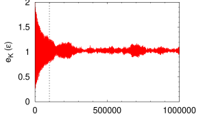
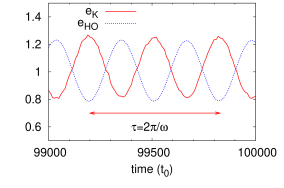
Figure 1: (Color online) Upper part: total kinetic energy per particle as a function of time (in Lennard-Jones units) for a Lennard-Jones system of 147 particles trapped in a harmonic oscillator of spring constant $k$ such that $\omega=\sqrt{k/m}=0.01t_{0}^{-1}$ for a total energy per particle $e=2.0\epsilon$. Lower part: zoom of the oscillation dynamics over a reduced time interval. Dashed line: potential energy associated to the collective oscillation $e_{HO}=\langle k\hat{r}^{2}/2\rangle$.

III.1 Dynamics of Lennard-Jones systems

Figure 1 shows a single very long molecular dynamics run for the Lennard-Jones particles trapped in a harmonic oscillator. Even if the amplitude of the initial oscillations is damped by the inter-particle interaction, it is apparent from Figure 1 that collective oscillations persist over extremely long times and the ergodic limit does not seem to be attained. This situation is virtually independent of the chosen collective frequency and total energy. As we now show, this behavior can be understood from the closed algebraic structure of the $\hat{p}^{2}$, $\hat{r}^{2}$ and $\hat{\vec{r}}\cdot\hat{\vec{p}}$ operators, which is preserved in classical mechanics if commutators are replaced by Poisson brackets.

Let us consider as above an initial condition given by eq.(1) within the ideal gas $\hat{H}=\hat{E}_{K}+k\hat{R}^{2}/2$ or diluted Boltzmann limit. If the only constraint on the size is given by the harmonic potential, the density matrix eq.(1) is a stationary solution of the Liouville equation. If conversely the system is initialized to a different average size through an extra constraint $\lambda_{0}\neq 0$, the system will evolve with the appearance of a collective flow $\hat{B}^{(1)}=-\sum_{n}\frac{1}{m}\left(\hat{\vec{p}}_{n}\cdot\hat{\vec{r}}_{n}+\hat{\vec{r}}_{n}\cdot\hat{\vec{p}}_{n}\right)$ as in eq.(6). Contrary to the free case, the successive constraining operators $\hat{B^{(p)}}$ do not vanish for any $p\geq 1$ and can be written as

$$\hat{B}^{(2p)} = \sum_{i=1}^{N}(-1)^{p}\left(2\omega\right)^{2p}\left(\frac{\hat{r}_{i}^{2}}{2}-\frac{\hat{p}_{i}^{2}}{2mk}\right)$$ (15)

$$\hat{B}^{(2p+1)} = -\sum_{i=1}^{N}(-1)^{p}\left(2\omega\right)^{2p}\frac{\hat{\vec{p}}_{i}\cdot\hat{\vec{r}}_{i}+\hat{\vec{r}}_{i}\cdot\hat{\vec{p}}_{i}}{m}$$ (16)

with $\omega=\sqrt{k/m}$. This gives at any time a density matrix with the same functional form as eq.(8), with an effective temperature $\tilde{\beta}$, constraining field $\tilde{\lambda}$, and collective radial velocity $\tilde{\nu}$ oscillating in time. For the purpose of getting analytical results it is easier to consider an initial condition in the canonical ensemble

$$\hat{D}_{\beta_{0},\lambda_{0}}\left(t_{0}\right)=\frac{1}{Z_{\beta_{0},\lambda_{0}}}\exp\left(-\beta_{0}\hat{H}-\lambda_{0}\hat{R}^{2}\right).$$ (17)

The series eq.(3) can be analytically summed up, and the time dependent partition sum results $Z_{\tilde{\beta},\tilde{\lambda},\tilde{\nu}}=z_{\tilde{\beta},\tilde{\lambda},\tilde{\nu}}^{N}$ with

$$z_{\tilde{\beta},\tilde{\lambda},\tilde{\nu}}(t) = Tr\Bigl{[}\exp\Bigl{(}-\tilde{\beta}\left(t\right)\frac{\hat{p}^{2}}{2m}-\tilde{\lambda}\left(t\right)\hat{r}^{2}$$ (18)

$$+ \frac{\tilde{\nu}\left(t\right)}{2}\left(\hat{\vec{p}}\cdot\hat{\vec{r}}+\hat{\vec{r}}\cdot\hat{\vec{p}}\right)\Bigr{)}\Bigr{]},$$

The time dependent Lagrange parameters are given by

$$\tilde{\beta}\left(t\right) = \beta_{0}-\frac{\lambda_{0}}{k}\left(\cos 2\omega\Delta t-1\right)$$ (19)

$$\tilde{\lambda}\left(t\right) = \frac{1}{2}\left(\beta_{0}k+\lambda_{0}\left(\cos 2\omega\Delta t+1\right)\right)$$ (20)

$$\tilde{\nu}\left(t\right) = \frac{\lambda_{0}}{m\omega}\sin 2\omega\Delta t.$$ (21)

Eq.(18) can be interpreted as a Gibbs equilibrium in the rest frame of a breathing system. For classical particles the trace over single-particle microstates is a phase-space integral $Tr[]=h^{-3}\int d^{3}r\int d^{3}p$ and the canonical partition sum is readily evaluated

$$z_{\tilde{\beta},\tilde{\lambda},\tilde{\nu}}(t)=\frac{2\sqrt{\pi}m}{h^{3}}\left(2\tilde{\beta}\tilde{\lambda}-\tilde{\nu}^{2}m\right)^{-3/2}$$ (22)

This leads to the prediction for the time dependent behavior of the different observables

$$\frac{\langle p^{2}\rangle}{2m} = -\frac{\partial\log z_{\tilde{\beta}\tilde{\lambda}\tilde{\nu}}}{\partial\tilde{\beta}}=\frac{6m\tilde{\lambda}}{2\tilde{\beta}\tilde{\lambda}-\tilde{\nu}^{2}m}$$ (23)

$$\langle r^{2}\rangle = -\frac{\partial\log z_{\tilde{\beta}\tilde{\lambda}\tilde{\nu}}}{\partial\tilde{\lambda}}=\frac{3\tilde{\beta}}{2\tilde{\beta}\tilde{\lambda}-\tilde{\nu}^{2}m}$$ (24)

$$\langle\vec{p}\cdot\vec{r}\rangle = \frac{\partial\log z_{\tilde{\beta}\tilde{\lambda}\tilde{\nu}}}{\partial\tilde{\nu}}=\frac{3m\tilde{\nu}}{2\tilde{\beta}\tilde{\lambda}-\tilde{\nu}^{2}m}$$ (25)

Introducing the expressions of $\tilde{\beta},\tilde{\lambda},\tilde{\nu}$ we get

$$e_{K}\equiv\frac{\langle p^{2}\rangle}{2m} = \frac{3}{2\beta_{0}}\frac{1+x\left(1+\cos 2\omega\Delta t\right)/2}{1+x}$$ (26)

$$e_{HO}\equiv\frac{k}{2}\langle r^{2}\rangle = \frac{3}{2\beta_{0}}\frac{1+x\left(1-\cos 2\omega\Delta t\right)/2}{1+x}$$ (27)

$$e_{flow}\equiv\omega\langle\vec{p}\cdot\vec{r}\rangle = \frac{3}{2\beta_{0}}\frac{x}{1+x}\sin 2\omega\Delta t$$ (28)

where $x=k_{0}/k$ measures the strength of the initial constraint. It is clear from the inspection of Figure 1 that over the time scale of a collective oscillation the interparticle interaction can be neglected, the total energy conservation constraint does not seem to play an important role, and the canonical free particles result eq.(18) appears fairly accurate. The kinetic energy do oscillate with the double of the oscillator frequency in phase opposition, this collective motion breaking the ergodicity of the dynamics.

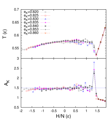
Figure 2: (Color online) Microcanonical temperature (upper part) and normalized kinetic energy fluctuation (lower part) as a function of the total energy inside the harmonic oscillator obtained from an energy sorting of canonical distributions corresponding to thermostat temperatures $\beta=3/(2e_{K})$ as indicated. All quantities are expressed in Lennard-Jones units.

III.2 Microcanonical Thermodynamics

In order to study the effect of flow for the freely expanding system, we have performed numerical molecular dynamics calculations within the statistical ensemble eq.(11) without ($h=0$) and with ($h>0$) the contribution of a radial collective flow. To study the thermodynamical properties of the isobar ensemble characterized by a size constraint $\lambda_{0}$ , we have constructed the microcanonical distribution by sorting a canonical ensemble Duflot of the equivalent system trapped in a harmonic oscillator of spring constant $k=2\lambda_{0}/\beta$. The canonical distributions are obtained by coupling the system to a thermostat with the Andersen technique Andersen . In brief, the coupling is made by stochastic impulsive forces that act occasionally on randomly selected particles. After each collision, the selected particle is endowed with a new velocity drawn from a Maxwell-Boltzmann distribution at the desired temperature $T$. The combination of Newtonian dynamics with the stochastic collisions generate a Markov chain in phase space, which under some general conditions generates the canonical distribution Andersen .

The resulting microcanonical thermodynamics is shown in Figure 2 for an oscillator constant $\omega=0.01t_{0}^{-1}$. Close to the liquid-gas transition temperature, the canonical calculations give rise to very wide energy distributions and the different events $(n)$ can be sorted in total energy bins

$$H_{n}=E_{Kn}+E_{LJn}+\frac{1}{2}kR^{2}_{n}$$ (29)

This energy can be physically interpreted as a free enthalpy for the isolated unbound system characterized by a finite size at the freeze-out time Duflot . Each single canonical sampling can therefore be used to access the microcanonical thermodynamics over a wide enthalpy region. The microcanonical temperature is evaluated in each enthalpy bin as $T(H)=2<e_{K}>/3$ noi where the average is taken over events belonging to the same bin. The normalized kinetic energy fluctuation $A_{K}=N\left(\langle e_{K}^{2}\rangle-\langle e_{K}\rangle^{2}\right)/T^{2}$ is also represented. The nice agreement between estimations obtained with different canonical temperatures shows the quality of the numerical sampling.

Figure 3: (Color online) Microcanonical temperature (upper part), normalized kinetic energy fluctuation (medium part) and mean square radius (lower part) as a function of the total energy inside the harmonic oscillator for two different oscillator strengths. The horizontal lines in the medium panels give the fluctuation expected in the canonical ensemble.

Figure 3 shows the dependence of the results on the oscillator strength. We can recognize for low $\omega$ values, $i.e.$ loose constraints on the system size, the first order liquid-gas phase transition. The transition is signaled by the backbending of the microcanonical caloric curve Gross corresponding to a negative heat capacity, and the associated abnormal kinetic energy fluctuation overcoming the canonical limit $A_{K}=3/2$ noi . The consistency between the two independent signals is again a proof of the numerical quality of the microcanonical sampling. These results are in qualitative agreement with the ones obtained for the Lattice Gas model in the same ensemble Duflot . We can also notice that in the energy interval corresponding to the transition, the mean square radius shows a kink and a slope change at higher energies. The spatial extension of the unbound phase grows more rapidly with the energy, and at the coexistence point the two phases have similar spatial extensions. This means that in this model, contrary to the Lattice case noi , the two coexisting phases at the transition temperature can be populated even in an ensemble which strongly constrains the volume of the system. In particular the two characteristic signals of a first order phase transition in a finite system, namely bimodality in the canonical ensemble and negative heat capacity in the microcanonical one, can be observed even in the isochore ensemble Chernomoretz ; Ariel .

For stronger size constraints (smaller average volumes) the caloric curve is monotonic, the microcanonical constraint reduces fluctuations well below the canonical limit, and the mean square radius increases linearly with the energy. This signals a supercritical system. From these calculations the critical pressure can be roughly estimated as $\omega_{c}\approx 0.015t_{0}^{-1}$.

IV MICROSTATE DISTRIBUTIONS IN AN EXPANDING ENSEMBLE

To simulate the expanding ensemble eq.(11), a radial momentum $\vec{p}_{r}=m\tilde{h}r\vec{u}_{r}$ is added to each particle and a microcanonical sorting is imposed on the total energy including flow $E^{\prime}=\sum_{i}(\vec{p}_{i}+\vec{p}_{ri})^{2}/(2m)+E_{LJ}$. The Hubble factor $\tilde{h}$ employed at different energies has been obtained from the measured collective velocity of the same system freely expanding in vacuum ($E_{flow}^{free}$) according to $h^{2}/2m<R^{2}>=E_{flow}^{free}$ Matias . Since the addition of flow trivially increases the total energy $E$, such that $E^{\prime}=\langle E_{th}\rangle+\langle E_{flow}\rangle>E$, the comparison between the calculations without flow at an energy $E$ and those of the ensemble including flow at an energy $E^{\prime}$ have to be made such that the average thermal energy of both systems are similar $\langle E_{th}\rangle=E$.

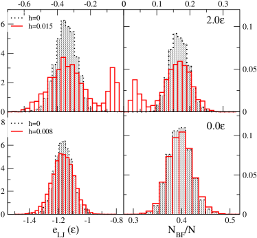
Figure 4: (Color online) Potential energy (left side) and size of the largest cluster (right side) at two different thermal energies corresponding to the bound phase (lower part) and close to the transition region (upper part). The filled histograms correspond to a static equilibrium $h=0$ while the empty ones flow was included according to eq.(11). All quantities are expressed in Lennard-Jones units.

The results are shown in Figure 4 for the distribution of the potential energy and the size of the largest fragment recognized through the MST algorithm Dorso . We can see that for all energies the presence of flow modifies the distributions in a sizeable way, leading to higher fluctuations. This is easy to understand from eq.(11) if we consider that in the expansion dynamics only the total energy is conserved, meaning that thermal energy fluctuations can be compensated by collective energy fluctuations. In this sense the collective motion acts as a heat bath, leading to distributions similar to the canonical ones. In particular if the system has a total energy inside the coexistence region of the first order phase transition (upper part of Figure 4) the exchange with the flow reservoir can allow the system to explore the two coexisting phases. These latter differ in potential energy $\Delta e_{LJ}\approx 0.4\epsilon$ but not in average spatial extension (see Figure 3) and can therefore be accessed in the same ensemble for a given value of the average freeze-out volume.

This result implies that signals of phase transitions typical of the canonical ensemble such as bimodalities can be pertinent also in the microcanonical framework, if flow is accounted for in a thermodynamical consistent way. Then such signals may be accessed even in experimental situations where the deposited energy is strongly constrained. A possible experimental confirmation of this prediction in nuclear multifragmentation can be found in ref.Pichon .

At this point a word of caution is in order. Our ansatz (11) is exact only for a system of non-interacting particles (or in the limit of local interactions). In the presence of strong correlations this ansatz supposes the system relaxation time be small compared to the time-scale of the expansion. This should be fulfilled if the average collective velocity $\langle v_{F}\rangle$ is much smaller than the velocity associated to the thermal motion $\langle v_{th}\rangle$. Within the ansatz (11) the local equation of state for the radial momentum reads

$$\langle p_{r}(r)\rangle\approx\frac{1}{r}\frac{\partial\log z}{\partial(\tilde{\beta}\tilde{h})}=\tilde{h}mr$$ (30)

where we have neglected the effect of the energy-conserving $\delta$-function in eq.(11) in order to have an analytical order-of-magnitude estimate. This leads to a collective velocity $v_{F}=\tilde{h}\langle R\rangle$ which should be compared to the canonical estimate $v_{th}=\sqrt{3/(\tilde{\beta}m)}$. In the case of the upper part of Figure 4 we have $v_{F}/v_{th}\approx 0.79$ meaning that the quality of our approximation may be doubtful. It is however interesting to note that the bimodal shape of the distribution in the presence of flow persists also for smaller collective motions, as long as the energy fluctuations are of the order of the energy distance $\Delta e_{LJ}$ between the two phases.

V CONCLUSIONS

To conclude, in this paper we have presented an information theory based formalism allowing to include collective motions in the statistical description of finite bound or unbound systems. Molecular dynamics simulations performed on a Lennard-Jones system suggest that even in the simplified approximation of non interacting particles, the presence of flow can influence the microstate distribution in a sizeable way. Indeed the presence of a (non-conserved in time) collective energy component can play the role of a heat bath, allowing for extra configurational energy fluctuations in the total energy conserving dynamics. In particular, close to a first order phase transition, this mechanism is seen to give rise to a characteristic bimodal behavior, similar to some recent experimental observations in nuclear multifragmentation.

References

- (1) C. Bréchignac, Ph. Cahuzac, B. Concina, J. Leygnier, Phys. Rev. Lett. 89, 203401 (2002)
- (2) M. Schmidt, T. Hippler, J. Donges, W. Kronm ller, B. von Issendorff, H. Haberland, P. Labastie, Phys. Rev. Lett. 87, 203402 (2001)
- (3) P. Brockhaus, K. Wong, K. Hansen, V. Kasperovich, G. Tikhonov, V. Kresin, Phys. Rev. A 59, 495, (1999)
- (4) G. Martinet et al., Phys. Rev. Lett. 93, 063401 (2004)
- (5) F. Gobet, B. Farizon, M. Farizon, M. J. Gaillard, J. P. Buchet, M. Carr , P. Scheier, T. D. M rk, Phys. Rev. Lett. 89, 183403 (2002)
- (6) K. Gluch, S. Matt-Leubner, O. Echt, B. Concina, P. Scheier, T. D. J. M rk, Chem. Phys. 121, 2137 (2004)
- (7) C. E. Klots, Nature (London) 327, 222 (1987)
- (8) F. Calvo, J. Phys. Chem. A 110, 1561 (2006)
- (9) “Dynamics and Thermodynamics with nuclear degrees of freedom”, Ph. Chomaz, F. Gulminelli, W. Trautmann and S. Yennello eds., Springer (2006)
- (10) W.Reisdorf, Prog. Theor. Phys. Suppl. 140, 111 (2000)
- (11) J. P. Bondorf, D. Idier and I. N. Mishustin, Phys. Lett. B 359, 261 (1995)
- (12) E. V. Shuryak, arXiv:hep-ph/0608177
- (13) L. W. Chen, C. M. Ko, Phys. Lett. B 634, 205 (2006)
- (14) V. N. Russkikh, Yu. B. Ivanov, Phys. Rev. C 74, 034904 (2006)
- (15) Z. W. Lin and C. M. Ko, Phys. Rev. Lett. 89, 202302 (2002); R. J. Fries, S. A. Bass, B. Muller, Phys. Rev. Lett. 94, 122301 (2005)
- (16) V. Koch, Nucl. Phys. A 715, 108 (2003)
- (17) F. Becattini, J. Phys. Conf. Ser. 5, 175 (2005)
- (18) J. Rafelski, J. Letessier, Eur. Phys. J. A 29, 107 (2006)
- (19) C. B. Das and S. Das Gupta, Phys. Rev. C 64, 041601(R) (2001)
- (20) Sh. Chikazumi, et al., Phys. Rev. C 63, 024602 (2001)
- (21) B. Elattari, J. Richert, P. Wagner and Y. M. Zheng, Nucl. Phys. A 592, 385 (1995)
- (22) Ph. Chomaz, F. Gulminelli and O. Juillet, Ann. Phys. 320, 135 (2005)
- (23) F. Becattini et al., Phys. Rev. C 73, 044905 (2006); A. Andronic, P. Braun-Munzinger, J. Stachel, Nucl. Phys. A 772, 167 (2006)
- (24) S. Pal, S. K. Samaddar and J. N. De, Nucl. Phys. A 608, 49 (1996)
- (25) S. K. Samaddar, J. N. De and S. Shlomo, Phys. Rev. C 69, 064615 (2004)
- (26) J. P. Bondorf, A. S. Botvina, A. S. Iljinov, I. N. Mishustin, K. Sneppen, Phys. Rep. 257, 133 (1995)
- (27) G. J. Kunde, et al., Phys. Rev. Lett. 74, 38 (1995)
- (28) W. Reisdorf et al., Phys. Lett. B 595, 118 (2004)
- (29) A. Strachan, C. O. Dorso, Phys. Rev. C 58, 632 (1998); Phys. Rev. C 59, 285 (1999)
- (30) A. Chernomoretz, F. Gulminelli, M. J. Ison, C. O. Dorso, Phys. Rev. C 69, 034610 (2004)
- (31) A. Chernomoretz, M. Ison, S. Ortiz, C. O. Dorso, Phys. Rev. C 64, 024606 (2001)
- (32) M. J. Ison and C. O. Dorso, Phys. Rev. C 71, 064603 (2005)
- (33) F. Gulminelli and Ph. Chomaz, Nucl. Phys. A 734, 581 (2004)
- (34) D. H. E. Gross, Lecture Notes in Physics vol.66, World Scientific (2001).
- (35) Ph. Chomaz and F. Gulminelli, in T. Dauxois et al., Lecture Notes in Physics Vol. 602, Springer (2002); F.Gulminelli, Ann. Phys. Fr. 29, 6 (2004)
- (36) F. Bouchet, J. Barré, Journ. Stat. Phys. 118, 1073 (2005)
- (37) M. D’Agostino et al., Phys. Lett. B 473, 219 (2000)
- (38) W. Norenberg, G. Papp and P. Rozmej, Eur. Phys. J. A 9, 327 (2000)
- (39) X. Campi, H. Krivine, N. Sator, Nucl. Phys. A 681, 458 (2001)
- (40) E. T. Jaynes, “Information theory and statistical mechanics”, Statistical Physics, Brandeis Lectures, vol.3, 160 (1963).
- (41) R. Balian, “From microphysics to macrophysics”, Springer Verlag (1982).
- (42) F. Gulminelli, Ph. Chomaz, O. Juillet, M. J. Ison and C. O. Dorso, AIP Conference Proceedings 884, 332 (2007); M.Ison et al., in preparation.
- (43) D. Frenkel and B. Smit, “Understanding molecular simulation”, Academic Press, Elsevier (1996)
- (44) A. C. Branka and K. W. Wojciechowski, Phys.Rev. E 62, 3281 (2000); F. Legoll et al., arXiv:math/0511178.
- (45) F. Gulminelli, Ph. Chomaz and V. Duflot, Europhys. Lett. 50, 434 (2000)
- (46) H. C. Andersen, Journ. Chem. Phys. 72, 2384 (1980)
- (47) N. Bellaize et al., Nucl. Phys. A 709, 367 (2002); P. Lautesse et al., Phys. Rev. C 71, 034602 (2005); M. Pichon et al., Nucl. Phys. A 779, 267 (2006)