When can Fokker-Planck Equation describe anomalous or chaotic transport ?

Abstract

The Fokker-Planck Equation, applied to transport processes in fusion plasmas, can model several anomalous features, including uphill transport, scaling of confinement time with system size, and convective propagation of externally induced perturbations. It can be justified for generic particle transport provided that there is enough randomness in the Hamiltonian describing the dynamics. Then, except for 1 degree-of-freedom, the two transport coefficients are largely independent. Depending on the statistics of interest, the same dynamical system may be found diffusive or dominated by its Lévy flights.

The Fokker-Planck Equation (FPE) is a basic model for the description of transport processes in several scientific fields. In one dimension it reads

$$\partial_{t}n(x,t)=-\partial_{x}\left({V(x)n}\right)+\partial_{x}^{2}\left({D(x)n}\right)$$ (1)

where $n$ is the density for a generic scalar quantity, $V$ the dynamic friction, and $D$ the diffusion coefficient. In particular, FPE backs up the diffusion-convection picture of anomalous transport in magnetized thermonuclear fusion plasmas, where $V$ is often referred to as a pinch velocity. This transport stems from turbulence triggered by density and temperature gradients through convective instabilities. Though very popular, the drift-diffusive picture underlying FPE breaks down in some cases. This was proved, e.g., for the transport of tracer particles suddenly released in pressure-gradient-driven turbulence, which exhibits strongly non gaussian features ref1 . This fact triggered a series of studies where transport was described in terms of continuous random walks with Lévy jumps, and of fractional diffusion models (see ref2 and references therein). This sets the issue: when is FPE relevant for anomalous or chaotic transport, when is it not?

Our discussion has many facets, but goes through the following main steps : (i) FPE with a source term can model phenomena commonly labeled as “anomalous” in fusion plasmas: uphill transport ref3 , anomalous scaling of confinement time with system size ref4 , and non diffusive propagation of externally induced perturbations ref5 . (ii) If the source is narrower than the mean random step of the true dynamics, FPE fails, while the correct Chapman-Kolmogorov equation reveals the existence of spatial features of the spreading quantity that are not related to the transport coefficients. (iii) For general 1 degree-of-freedom (dof) Hamiltonian dynamics, the constraint V = dD/dx holds, as originally derived by Landau. This constraint vanishes for higher dimensional dynamics, incorporating for instance particle-turbulence self-consistency, or the full 3-dimensional motion of particles. (iv) FPE can be justified for particle transport provided that there is enough randomness in the Hamiltonian describing the dynamics: e.g., when it includes many waves with random phases. This may work even whenever the dynamics of individual particles exhibit strong trapping motion. However chaos is not enough to justify FPE. (v) The diffusion may be quasilinear (QL) or not, depending on the so-called Kubo number $K$, which scales like the correlation time ref6 ; ref7 . For $K$ small, QL diffusion is due to the locality in velocity of wave-particle resonance. Large $K$ diffusion is due to the locality of trapping in phase-space.

Our discussion aims at providing insight in transport mechanisms, rationales for confinement scaling laws, and tools for experimental data analysis. It involves several building blocks: some are provided by the available literature, while a few are elaborated here. Though written for the fusion community, a large part of our discussion is of direct relevance to chaotic transport, and in particular to Lagrangian dynamics in incompressible turbulence.

What FPE can do. The case where $V$ and $D$ are constant in Eq. (1) is often considered in fusion data analysis. An initially Dirac-like perturbation travels with velocity V, while diffusing with coefficient $D$. For large enough systems, $L\gg D/V$, the perturbation actually travels ballistically. Thus FPE can model the non diffusive propagation of induced perturbations in a fusion machine ref5 . The scaling of confinement time $\tau_{\text{conf}}$ with system size $L$, goes from diffusive ($\tau_{\text{conf}}\propto L^{2}$, $L\ll D/V$) to ballistic ($\tau_{\text{conf}}\propto L^{1}$, $L\gg D/V$). Thus FPE may account for anomalous scaling of confinement time with system size. It is even more so when $V$ and $D$ depend on $x$ ref4 , or when their possible dependence on spatial gradients driving turbulence is accounted for. Whatever $V$ and $D$ be, FPE may be written as $\partial_{t}n=-\partial_{x}\Gamma$, with the flux $\Gamma=Vn-\partial_{x}(Dn)$ . For $D$ constant, if there are no sources in the central part of the plasma, for symmetry reasons $\Gamma=0$, which yields $\partial_{x}n/n=V/D$: if $sign(x)V<0$, where $x=0$ corresponds to the plasma center, the probability piles up toward small $|x|$’s, leading to an equilibrium distribution of “uphill transport” type ref3 . However, the piling up may result as well from $V=0$, and $D(x)$ growing with $|x|$ since $n(x)\propto 1/D(x)$. This is a caveat for data analysis: a broad family of $(V,D)$ profiles can model the same experimental data. Let us notice that the ability of FPE to describe anomalous transport is shared with models giving non gaussian features (see ref2 and references therein).

Transport in presence of a source. The classical derivation of FPE from the Chapman-Kolmogorov equation

$$\partial_{t}n(x,t)=\int P(x,x^{\prime}){n(x^{\prime},t)\over\tau(x^{\prime})}dx^{\prime}-{n(x,t)\over\tau(x)}+S(x),$$ (2)

where $S(x)$ is a localized source term and $\tau(x)$ is a waiting time, assumed to be 1 for the moment, assumes the typical width $\sigma_{P}$ of $P$ in $x-x^{\prime}$ to be the smallest spatial scale of interest. Therefore the width $\sigma_{S}$ of $S$ must be much larger than $\sigma_{P}$ for FPE to describe correctly $n(x,t)$ within the source domain; otherwise the source pumps strong gradients in $n(x,t)$, and the Taylor expansion leading to FPE breaks down close to it. Assume $P(x,x^{\prime})$ to be a function of $x-x^{\prime}$ only. Then Eq. (2) shows that for scales smaller than $\sigma_{P}$, the Fourier transform of a stationary $n(x)$ is almost equal to that of $S(x)$. These are the scales relevant to describe the profile close to the source. Therefore, $n(x)$ displays a bump similar to that of $S(x)$ that is not due to specific properties of the FPE transport coefficients: a further caveat for data analysis.

Paradigm model. Consider tracer transport in 2-dimensional (2D) incompressible turbulence, or transport in magnetized plasmas induced by electrostatic turbulence in the guiding center approximation. A paradigm for such a transport is the equation of motion

$$\frac{{d{\bf{X}}}}{{dt}}=-\nabla\Phi({\bf{X}},t)\times{\bf{\hat{x}}}_{3}\equiv{\bf{v}}$$ (3)

with ${\bf{X}}=(x_{1},x_{2})$ the particle position (perpendicular to the magnetic field, for the plasma case) and $\Phi$ the flow function or the appropriately normalized electrostatic potential. Model (3) applies to transport due to magnetic chaos as well. Indeed, for an almost straight magnetic field, $\Phi$ may be replaced by $\Phi^{\prime}=\Phi-v_{||}A_{||}$, where both the electrostatic potential $\Phi{}$ and the parallel vector potential $A_{||}$ are computed at the guiding center position, and $v_{||}$ is the parallel velocity ref6 . Therefore Eq. (3) describes the canonical equations for the guiding center dynamics in a mixture of electrostatic and magnetostatic fields, ruled by Hamiltonian $\Phi(\bf{X},\rm{t})$, with conjugate variables $x_{1}$ and $x_{2}$.

Constraint on FPE due to the dimensionality. Consider model (3) where $\Phi$ has a bounded support, or is periodic in the $x_{i}$’s with an elementary periodicity cell $R$: motion is, or can be considered as, located within a bounded domain $R$ of phase space. Because of conservation of the area of a phase space element during motion, an initially uniform particle density $n$ in $R$ must remain uniform for later times. Now, assume FPE describes the evolution of $n(x)$ ($x$ one of the two conjugate variables). Since $n$ is stationary, the flux $\Gamma$ must be a constant in $R$, and must vanish, since it does on the boundary of $R$. Since $\Gamma=Vn-\partial_{x}(Dn)$, this requires $V=dD/dx$. This is the fundamental reason for this constraint, first derived by Landau ref8 for a stochastic but non chaotic Hamiltonian dynamics, since his derivation uses Taylor expansions of the orbit in time. The Landau constraint (LC) was recovered more recently for the chaotic motion of particles in a prescribed set of Langmuir waves ref10 . If $V=dD/dx$, then $\Gamma=-Ddn/dx$. In absence of sources in the plasma core, $\Gamma{}=0$ implies $dn/dx=0$ in this domain, which rules out uphill transport.
Adding more dimensions to the previous Hamiltonian dynamics (for instance the parallel motion in addition to the E$\times$B drift) leads in general to a breakdown of LC. Indeed a Kolmogorov-Arnold-Moser torus is no longer able to separate the chaotic domain into disconnected sets (Arnold diffusion), and therefore there are no longer boundaries $\Gamma$ must vanish onto. For instance, LC no longer holds for the self-consistent motion of particles in a set of Langmuir waves (here $x$ is the particle velocity): $V$ is equal to $dD/dx$ plus a drag force due to the spontaneous emission of waves by particles ref10 . The analogy of Langmuir wave-electron interaction with the toroidal Alfven eigenmode-fast ion one, where $x$ is the radial position ref11 , shows that a similar effect may hold for a fusion machine. This is a particular instance revealing that the true Hamiltonian dynamics of particles in fusion machines has more than 1 dof. In general LC cannot hold then: uphill transport and a central finite density gradient are possible.

Derivation of FPE from Hamiltonian dynamics for particles. We consider model (3) where $\Phi$ is a statistically stationary, spatially homogeneous, isotropic zero-mean-value stochastic potential with typical amplitude $\Phi_{0}$, and a given two-point, two-time correlation function, with correlation time $\tau_{c}$ and correlation length $\lambda_{c}$, as considered in Refs. ref6 ; ref12 . Some results from these references are important for justifying FPE in this case. Potential $\Phi$ drives the particles motion by setting the instantaneous value of their velocity, whose typical amplitude is $\Phi_{0}/\lambda_{c}$. The system chooses among two types of diffusive chaotic dynamics according to the value of the Kubo number $K=\Phi_{0}\tau_{c}/\lambda_{c}^{2}$. The rationale for this is the following. If the potential is static ($\tau_{c}$ infinite), particles are trapped into potential wells and hills, and possibly make long flights along “roads” crossing the whole chaotic domain. These various domains are separated by separatrices joining nearby hyperbolic points. If $\tau_{c}$ is finite, but large ($K\gg 1$), the potential topography slowly changes, and the dynamics evolves quasi-adiabatically. Since phase space area inside the instantaneous closed orbits must be adiabatically preserved, and since the area of the various domains defined by the separatrix array fluctuates a lot, orbits must cross the instantaneous separatrices, and jump this way from one domain to the next one (Fig. 1(a)) . In the absence of “roads”, which is almost the case for a gaussian spatial correlation function of the potential ref12 , these crossings produce a random walk with step $\lambda_{c}$ and waiting time $\tau_{c}$; the corresponding diffusion coefficient is $D\approx\lambda_{c}^{2}/\tau_{c}$. The presence of “roads” modifies this estimate and brings some dependence upon $K$ ref12 . As a result, for $K\gg 1$ diffusion is justified by locality of trapping in phase-space.

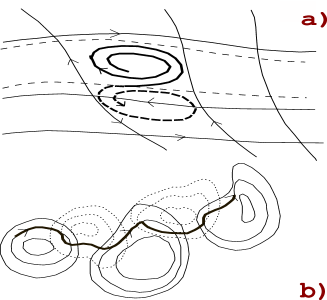
Figure 1: (a) $K\gg 1$: as the net of intersecting separatrices evolves in time (from solid to dashed curves), the lower domain enlarges at the expense of the upper one. Hence a trajectory may go from the upper to the lower one (thick to dashed curve). (b) $K\ll 1$: jumps among small trapping arcs in a quickly evolving potential topography. Solid and dashed contours stand for potential hills and wells.

When $K\ll 1$, the particles typically run only along a small arc of length $\Phi_{0}\tau_{c}/\lambda_{c}$ of the trapped orbits of the instantaneous potential during a correlation time. During the next correlation time they perform a similar motion in a potential completely uncorrelated with the previous one (Fig. 1(b)). These uncorrelated random steps yield a 2D Brownian motion with a QL diffusion coefficient $D\approx\Phi_{0}^{2}\tau_{c}/\lambda_{c}^{2}$. These two limit cases in $K$ show diffusion is a quite general behavior of particle transport, even whenever structures are visible in the electrostatic potential, or whenever non gaussian behaviour is obtained for a more limited statistics, as in Ref. ref1 whose dynamics, except for isotropy, may be thought as one realization of that in Ref. ref12 .

The simple preceding reasoning strongly bears on the stochastic properties of the potential, and not on the chaotic features of particle dynamics. A more rigorous picture for the diffusion process of the $K\ll 1$ regime can be given, which incorporates chaos as an essential ingredient, but exhibits the paramount importance of potential randomness. This picture is a translation for dynamics (3) of that described in Refs. ref10 ; ref14 for the dynamics of an electron in a set of Langmuir waves. To this end, we consider $\Phi$ as a sum of propagating modes $\varepsilon a_{{\bf{k}},\omega}\cos\left({{\bf{k}}\cdot{\bf{X}}-\omega t+\varphi_{{\bf{k}},\omega}}\right)$, where the $\varphi_{\bf{k},\omega}$’s are uniformly distributed random phases, and the spectrum is isotropic in $\bf{k}$; $\varepsilon$ is put for scaling purposes. If the particle does not resonate with the modes in (3), its dynamics may be described by perturbation theory in $\varepsilon$. In the opposite case, at any given time $t_{0}$ where the particle has velocity $\textbf{v}(t_{0})$, some modes are resonant with the particle, and their action cannot be described in a perturbative way, but some are not, and still act perturbatively. These two classes can be defined according to their resonance mismatch with the particle $\rho(t_{0})=\left|{\textbf{k}\cdot\textbf{v}(t_{0})-\omega}\right|$ ref10 ; ref14 ; ref15 . Consequently, the instantaneous particle motion splits into a perturbative, and thus non chaotic part, and into a non perturbative chaotic part due to the set $S(\textbf{v}(t_{0}))$ of modes which are resonant enough with the particle at time $t_{0}$: $\rho(t_{0})$ less than some threshold $\rho_{0}\sim\varepsilon$. This set evolves with time, according to the instantaneous value of $\textbf{v}(t)$. A suitable choice of $\rho_{0}/\varepsilon$ enables to incorporate the set of modes driving the chaotic dynamics of the particle over a finite interval $[t_{0}-\Delta t,t_{0}+\Delta t]$, where $\Delta t$ is of the order of the time $\tau_{\text{spread}}\approx\lambda_{c}^{2}/D$. Over this time interval the chaotic particle dynamics is ruled by a reduced Hamiltonian $\Phi_{t_{0}}(\textbf{X},t)$, which is $\Phi(\textbf{X},t)$ with the summation restricted over the modes inside set $S(\textbf{v}(t_{0}))$. If the dynamics is chaotic, $\textbf{v}(t)$ changes a lot its direction during its motion, which brings disconnected sets $S(\textbf{v}(t_{n}))$, for different times $t_{n},n=0,1,...$. The randomness of the $\varphi_{\bf{k},\omega}$’s implies that the dynamics ruled by each of the $\Phi_{t_{n}}({\bf{X}},t)$’s are statistically independent, which justifies a central limit argument for their cooperative contribution to the particle motion: the dynamics is indeed diffusive.
The above argument uses the locality of wave-particle resonance in phase velocity. It also holds to prove the diffusive behavior for peaked frequency spectrum, or for a single typical outcome of the random phases, if the set of the initial particle velocities $\textbf{v}_{0}$ is spread enough for them to be acted upon by a large number of disconnected $S(\textbf{v}_{0})$’s. This explains the diffusive behavior found in ref16 by averaging over initial particle positions. It should be stressed that the above locality rationale depends essentially on the random phases, and that chaos, through the breakup of KAM tori, just brings in the ability of the motion to be ruled successively by uncorrelated dynamics. In the absence of random phases no diffusivity can be derived by the above reasoning. Indeed the diffusion picture was clearly shown to break down in ref1 , and for electron dynamics due to Langmuir waves ref15 .
The existence of random phases can also be used to derive a rigorous QL estimate for $D$. This derivation is analogous to that for the chaotic dynamics due to Langmuir waves for $K\ll 1$ ref10 . Its central argument is that the dynamics depends slightly on any two phases during a time much larger than $\tau_{\text{spread}}$, which defines the time of strong sensitivity of the dynamics on the whole set of random phases ref14 . These successive two random-phase arguments for the $K\ll 1$ case, assumed for simplicity that all phases were uncorrelated, but some correlation may be accommodated. We stress they do not use at all any loss of memory due to chaotic motion: indeed differentiable chaotic Hamiltonian dynamics is not hyperbolic.

Beyond simple Hamiltonian models. More recently Vlad et al. ref17 introduced a spatial inhomogeneity in model (3), such that its r.h.s. is multiplied by a growing function of $x_{1}$. This was meant as a modeling of the increase of the magnetic field toward the main axis of a fusion machine, but makes the dynamics non Hamiltonian stricto sensu. On top of the previous diffusive behavior (which becomes anisotropic), the new inhomogeneity brings a “radial” drift velocity $V$ along $x_{1}$ due to the chaotic motion, which corresponds to the dynamic friction of FPE. The sign of $V$ depends on $K$. If $K\ll 1$, since the velocity increases toward larger $x_{1}$’s, the displacement during a correlation time is larger toward the exterior than toward the interior, which brings an outgoing drift. If $K\gg 1$, the trapped particles are slower in the inner part of their orbit, which increases their probability to be there with respect to that to be in the outer part: this brings an ingoing drift. Since $D$ now grows with $x_{1}$, $V=dD/dx_{1}$ is impossible for $K\gg 1$.
The previous discussion can be extended to higher dimensional systems quite naturally, as do the above arguments of locality, or the argument of the weak effect of two phases on the dynamics. The diffusive aspect of higher dof chaotic systems is largely documented as well (see ref17b and references therein). In conclusion we may state that depending on the statistics of interest, the same dynamical system may be found diffusive or dominated by its Lévy flights. In particular averaging over many random phases may lead to diffusion, while averaging only over a limited set of initial conditions for the particles may lead to the Lévy flight picture. Since fusion experiments generally average over many plasma realizations, and global confinement scaling laws even more so, FPE is a highly relevant tool for this field. It should be noted that in a magnetized toroidal plasma, density $n$ describing particle transport is the true particle density divided by a growing function $\tau(x)$ of the local magnetic field (see ref17c and references therein). This brings a slanting of the density profile toward the outer part of the torus that has nothing to do with a turbulent transport phenomenon, in contrast with that in Ref. ref17 , and which corresponds exactly to a waiting time $\tau(x)$ in Eq. (2). This is one more caveat for data analysis.
We found that for $K\ll 1$, FPE with a QL diffusion coefficient is justified by chaotic Hamiltonian dynamics with random phases, even though structures exist in phase space for one realization of the phases. This, and the fact that the QL diffusive modeling of transport is quite efficient ref18 , suggest that $K$ is small in magnetic fusion turbulence. There are reasons for $K$ not to be large. First, the usual estimate in fluid mechanics of the correlation time as the eddy turn-over time yields $K=1$ ref18b . Furthermore strong turbulence theory predicts that $K$ is at most of order 1 (see Eq. 4.34 of ref19 ). However the issue of the typical value of $K$ is still unsettled, since an analysis of fluctuation data in the TEXT tokamak indicated $K$ of order 1, and a poor agreement of QL estimates for impurity transport ref19b . It would be interesting to systematically compute $K$ from experimental or numerical data. In rotating or stratified fluid turbulence a weak effect of structures holds as well: cigar-like or pancake-like structures are present, but turbulent diffusion is correctly modeled by assuming random phases for the Fourier components of the turbulent fluid ref20 .

- (1) D. del-Castillo-Negrete, B.A. Carreras, and V.E. Lynch, Phys. Plasmas 11, 3854 (2004)
- (2) D. del-Castillo-Negrete, Phys. Plasmas 13, 082308 (2006)
- (3) C.C. Petty and T.C. Luce, Nucl. Fusion 34, 121 (1994); M.R. de Baar et al., Phys. Plasmas 6, 4645 (1999)
- (4) C.C. Petty, et al., Phys. Plasmas 2, 2342 (1995)
- (5) P. Mantica and F. Ryter, C. R. Physique 7, 634 (2006)
- (6) M. Ottaviani, Europhys. Lett. 20, 111 (1992)
- (7) M. Vlad et al., Phys. Rev. E 58, 7359 (1998)
- (8) L.D. Landau, Zh. Eksper. Theor. Fiz. 7, 203 (1937); A.J. Lichtenberg and M.A. Lieberman, Regular and Stochastic Motion (Springer-Verlag, 1983)
- (9) Y. Elskens and D. Escande, Microscopic Dynamics of Plasmas and Chaos (Institute of Physics Publishing, 2003); Phys. Lett. A 302, 110 (2002)
- (10) H.L. Berk and B.N. Breizman, Phys. Fluids B 2, 2246 (1990); N.J. Fisch and J.-M. Rax, Phys. Rev. Lett. 69, 612 (1992)
- (11) M. Vlad, et al., Plasma Phys. Control. Fusion 46, 1051 (2004)
- (12) D. Bénisti and D.F. Escande, Phys. Plasmas 4, 1576 (1997); J. Stat. Phys. 92, 909 (1998)
- (13) D. Bénisti and D.F. Escande, Phys. Rev. Lett. 80, 4871 (1998)
- (14) G. Ciraolo et al., J. Nucl. Mater. 363-365, 550 (2007)
- (15) M. Vlad, F. Spineanu, and S. Benkadda, Phys. Rev. Lett. 96, 085001 (2006)
- (16) M. Vlad et al., Plasma Phys. Control. Fusion 47, 281 (2005)
- (17) X. Garbet, et al., Phys. Plasmas 12, 082511 (2005)
- (18) R. Waltz, et al., Phys. Plasmas 4, 2482 (1997); J. Weiland, Collective Modes in Inhomogeneous Plasmas (Institute of Physics, Bristol, 2000).
- (19) M. Ottaviani, private communication
- (20) A. Yoshizawa et al., Plasma Phys. Control. Fusion 43, R1 (2001)
- (21) W. Horton and W. Rowan, Phys. Plasmas 1, 901 (1994)
- (22) C. Cambon et al., J. Fluid Mech. 499, 231 (2004)