Abstract

In this article, we study the vertices $DDV$ and $D^{*}DV$ with the light-cone QCD sum rules. The strong coupling constants $g_{DDV}$ and $f_{D^{*}DV}$ play an important role in understanding the final-state re-scattering effects in the hadronic $B$ decays. They are related to the basic parameters $\beta$ and $\lambda$ respectively in the heavy quark effective Lagrangian, our numerical values are smaller than the existing estimations.

PACS numbers: 12.38.Lg; 13.20.Fc

Key Words: Strong coupling constants, light-cone QCD sum rules

1 Introduction

Final-state interactions (or re-scattering effects) play an important role in the hadronic $B$ decays [1, 2]. However, it is very difficult to take them into account in a systematic way due to the nonperturbative nature of the multi-particle dynamics. In practical calculations, we can resort to phenomenological models to outcome the difficult. The one-particle-exchange model is typical (for example, see Ref.[2]), in this picture, the soft re-scattering of the intermediate states in two-body channels with one-particle exchange makes the main contributions. The phenomenological Lagrangian contains many input parameters, which describe the strong couplings among the charmed mesons in the hadronic $B$ decays.

In the following, we write down the relevant phenomenological Lagrangian, which describes the strong interactions of the $DDV$ and $D^{*}DV$ [2],

$$\mathcal{L} = ig_{DDV}D_{i}(\overrightarrow{\partial_{\mu}}-\overleftarrow{\partial_{\mu}})D_{j}V^{\mu}_{ij}$$

$$+2f_{D^{*}DV}\epsilon_{\mu\nu\alpha\beta}\partial^{\mu}V^{\nu}_{ij}\left[D_{i}\left(\overrightarrow{\partial^{\alpha}}-\overleftarrow{\partial^{\alpha}}\right)D^{*\beta}_{j}-D^{*\beta}_{i}\left(\overrightarrow{\partial^{\alpha}}-\overleftarrow{\partial^{\alpha}}\right)D_{j}\right]\,,$$

$$D = (D^{0},D^{+},D_{s})\,,$$

$$D^{*} = (D^{*0},D^{*+},D^{*}_{s})\,,$$

$$V = \left(\begin{array}[]{ccc}\frac{\rho^{0}}{\sqrt{2}}+\frac{\omega}{\sqrt{2}}&\rho^{+}&K^{*+}\\ \rho^{-}&-\frac{\rho^{0}}{\sqrt{2}}+\frac{\omega}{\sqrt{2}}&K^{*0}\\ K^{*-}&\bar{K}^{*0}&\phi\end{array}\right)\,.$$ (4)

The strong coupling constants $g_{DDV}$ and $f_{D^{*}DV}$ in the phenomenological Lagrangian can be related to the basic parameters $\beta$ and $\lambda$ in the heavy quark effective Lagrangian (one can consult Ref.[3] for the heavy quark effective Lagrangian and relevant parameters. ),

$$g_{DDV} = \frac{\beta g_{V}}{\sqrt{2}}\,,$$

$$f_{D^{*}DV} = \frac{\lambda g_{V}}{\sqrt{2}}\,,$$ (5)

where $g_{V}=5.8$ from the vector meson dominance theory [4].

In this article, we study the strong coupling constants $g_{DDV}$ and $f_{D^{*}DV}$ with the light-cone QCD sum rules [5, 6]. The strong coupling constants $g_{BB\rho}$, $g_{DD\rho}$, $f_{B^{*}B\rho}$ and $f_{D^{*}D\rho}$ have been calculated with the light-cone QCD sum rules in Ref.[7], I failed to take notice of that work at beginning.

The light-cone QCD sum rules carry out operator product expansion near the light-cone, $x^{2}\approx 0$, instead of short distance, $x\approx 0$, while the nonperturbative matrix elements are parameterized by the light-cone distribution amplitudes (which are classified according to their twists) instead of the vacuum condensates [5, 6]. The nonperturbative parameters in the light-cone distribution amplitudes are calculated by the conventional QCD sum rules and the values are universal [8].

The article is arranged as: in Section 2, we derive the strong coupling constants $g_{DDV}$ and $f_{D^{*}DV}$ with the light-cone QCD sum rules; in Section 3, the numerical result and discussion; and in Section 4, conclusion.

2 Strong coupling constants $g_{DDV}$ and $f_{D^{*}DV}$ with light-cone QCD sum rules

We study the strong coupling constants $g_{DDV}$ and $f_{D^{*}DV}$ with the two-point correlation functions $\Pi_{ij}(p,q)$ and $\Pi^{ij}_{\mu}(p,q)$,

$$\Pi_{ij}(p,q) = i\int d^{4}x\,e^{-iq\cdot x}\,\langle 0|T\left\{J_{i}(0)J_{j}^{+}(x)\right\}|V_{ij}(p)\rangle\,,$$ (6)

$$\Pi^{ij}_{\mu}(p,q) = i\int d^{4}x\,e^{-iq\cdot x}\,\langle 0|T\left\{J^{i}_{\mu}(0)J_{j}^{+}(x)\right\}|V_{ij}(p)\rangle\,,$$ (7)

$$J_{i}(x) = {\bar{q}}_{i}(x)i\gamma_{5}c(x)\,,$$

$$J^{i}_{\mu}(x) = {\bar{q}}_{i}(x)\gamma_{\mu}c(x)\,,$$ (8)

where the currents $J_{i}(x)$ interpolate the pseudoscalar mesons $D^{0}$, $D^{+}$, $D_{s}$ and the currents $J^{i}_{\mu}(x)$ interpolate the vector mesons $D^{*0}$, $D^{*+}$, $D^{*}_{s}$. The external states $\rho$, $K^{*}$ and $\phi$ have the four momentum $p_{\mu}$ with $p^{2}=m_{\rho}^{2}$, $m_{K^{*}}^{2}$ and $m_{\phi}^{2}$, respectively.

According to the basic assumption of current-hadron duality in the QCD sum rules [8], we can insert a complete series of intermediate states with the same quantum numbers as the current operators $J_{i}(x)$ and $J^{i}_{\mu}(x)$ into the correlation functions $\Pi_{ij}(p,q)$ and $\Pi^{ij}_{\mu}(p,q)$ to obtain the hadronic representation. After isolating the ground state contributions from the pole terms of the mesons $D_{i}$ and $D^{*}_{i}$, we get the following results,

$$\Pi_{ij}(p,q) = \frac{f_{D_{i}}f_{D_{j}}M_{D_{i}}^{2}M_{D_{j}}^{2}g_{D_{i}D_{j}V_{ij}}}{(m_{i}+m_{c})(m_{j}+m_{c})\left\{M_{D_{i}}^{2}-(q+p)^{2}\right\}\left\{M_{D_{j}}^{2}-q^{2}\right\}}2\epsilon\cdot q+\cdots$$ (9)

$$= \Pi^{P}_{ij}(p,q)\epsilon\cdot q+\cdots,$$

$$\Pi^{ij}_{\mu}(p,q) = \frac{f_{D^{*}_{i}}f_{D_{j}}M_{D_{i}^{*}}M_{D_{j}}^{2}g_{D^{*}_{i}D_{j}V_{ij}}}{(m_{j}+m_{c})\left\{M_{D^{*}_{i}}^{2}-(q+p)^{2}\right\}\left\{M_{D_{j}}^{2}-q^{2}\right\}}4\epsilon_{\mu\nu\alpha\beta}\epsilon^{\nu}p^{\alpha}q^{\beta}+\cdots$$ (10)

$$= \Pi^{V}_{ij}(p,q)\epsilon_{\mu\nu\alpha\beta}\epsilon^{\nu}p^{\alpha}q^{\beta}+\cdots,$$

where the following definitions for the weak decay constants have been used,

$$\langle 0|J_{i}(0)|D_{i}(p)\rangle = \frac{f_{D_{i}}M_{D_{i}}^{2}}{m_{i}+m_{c}}\,,$$

$$\langle 0|J^{i}_{\mu}(0)|D^{*}_{i}(p)\rangle = f_{D^{*}_{i}}M_{D^{*}_{i}}\epsilon_{\mu}\,.$$ (11)

In Eqs.(6-7), we have not shown the contributions from the high resonances and continuum states explicitly as they are suppressed due to the double Borel transformation.

In the following, we briefly outline operator product expansion for the correlation functions $\Pi_{ij}(p,q)$ and $\Pi_{\mu}^{ij}(p,q)$ in perturbative QCD theory. The calculations are performed at large spacelike momentum regions $(q+p)^{2}\ll 0$ and $q^{2}\ll 0$, which correspond to small light-cone distance $x^{2}\approx 0$ required by validity of operator product expansion. We write down the propagator of a massive quark in the external gluon field in the Fock-Schwinger gauge firstly [9],

$$\langle 0|T\{q_{i}(x_{1})\,\bar{q}_{j}(x_{2})\}|0\rangle = i\int\frac{d^{4}k}{(2\pi)^{4}}e^{-ik(x_{1}-x_{2})}\frac{\not\!k+m}{k^{2}-m^{2}}+\cdots\,,$$ (12)

where we have neglected the contributions from the gluons $G_{\mu\nu}$. The contributions proportional to $G_{\mu\nu}$ can give rise to three-particle (and four-particle) meson distribution amplitudes with a gluon (or quark-antiquark pair) in addition to the two valence quarks, their corrections are usually not expected to play any significant roles. Substituting the above $c$ quark propagator and the corresponding $\rho$, $K^{*}$, $\phi$ mesons light-cone distribution amplitudes into the correlation functions $\Pi_{ij}(p,q)$, $\Pi_{\mu}^{ij}(p,q)$ in Eqs.(3-4) and completing the integrals over the variables $x$ and $k$, finally we obtain the results,

$$\Pi^{P}_{ij} = f_{V_{ij}}m_{V_{ij}}\int_{0}^{1}du\frac{\phi_{\parallel}(u)}{AA}+\left[f_{V_{ij}}^{\perp}-f_{V_{ij}}\frac{m_{i}+m_{j}}{m_{V_{ij}}}\right]m_{c}m_{V_{ij}}^{2}\int_{0}^{1}du\frac{h_{||}^{(s)}(u)}{AA^{2}}$$ (13)

$$-\frac{f_{V_{ij}}m_{V_{ij}}^{3}}{4}\int_{0}^{1}duA(u)\left[\frac{1}{AA^{2}}+\frac{2m_{c}^{2}}{AA^{3}}\right]$$

$$-2f_{V_{ij}}m_{V_{ij}}^{3}\int_{0}^{1}du\int_{0}^{u}d\tau\int_{0}^{\tau}dtC(t)\left[\frac{1}{AA^{2}}+\frac{2m_{c}^{2}}{AA^{3}}\right]+\cdots\,,$$

$$\Pi^{V}_{ij} = f_{V_{ij}}^{\perp}\int_{0}^{1}du\frac{\phi_{\perp}(u)}{AA}-\frac{f_{V_{ij}}^{\perp}m_{V_{ij}}^{2}}{4}\int_{0}^{1}duA_{\perp}(u)\left[\frac{1}{AA^{2}}+\frac{2m_{c}^{2}}{AA^{3}}\right]$$ (14)

$$+\left[f_{V_{ij}}-f_{V_{ij}}^{\perp}\frac{m_{i}+m_{j}}{m_{V_{ij}}}\right]\frac{m_{c}m_{V_{ij}}}{2}\int_{0}^{1}du\frac{g_{\perp}^{(a)}(u)}{AA^{2}}+\cdots\,,$$

where

$$AA = m_{c}^{2}-(q+u\,p)^{2}\,.$$

In calculation, the two-particle vector mesons light-cone distribution amplitudes have been used [10], the explicit expressions are given in the appendix. The parameters in the light-cone distribution amplitudes are scale dependent and can be estimated with the QCD sum rules [10]. In this article, the energy scale $\mu$ is chosen to be $\mu=1\rm{GeV}$.

Now we perform the double Borel transformation with respect to the variables $Q_{1}^{2}=-(p+q)^{2}$ and $Q_{2}^{2}=-q^{2}$ for the correlation functions $\Pi_{ij}^{P}$ and $\Pi_{ij}^{V}$ in Eqs.(6-7), and obtain the analytical expressions of the invariant functions in the hadronic representation,

$$B_{M_{2}^{2}}B_{M_{1}^{2}}\Pi^{P}_{ij} = \frac{2g_{D_{i}D_{j}V_{ij}}f_{D_{i}}f_{D_{j}}M_{D_{i}}^{2}M_{D_{j}}^{2}}{(m_{c}+m_{i})(m_{c}+m_{j})M_{1}^{2}M_{2}^{2}}\exp\left[-\frac{M^{2}_{D_{i}}}{M_{1}^{2}}-\frac{M^{2}_{D_{j}}}{M_{2}^{2}}\right]+\cdots,$$ (15)

$$B_{M_{2}^{2}}B_{M_{1}^{2}}\Pi^{V}_{ij} = \frac{4f_{D_{i}^{*}D_{j}V_{ij}}f_{D^{*}_{i}}f_{D_{j}}M_{D^{*}_{i}}M_{D_{j}}^{2}}{(m_{c}+m_{j})M_{1}^{2}M_{2}^{2}}\exp\left[-\frac{M^{2}_{D_{i}^{*}}}{M_{1}^{2}}-\frac{M^{2}_{D_{j}}}{M_{2}^{2}}\right]+\cdots,$$ (16)

where we have not shown the contributions from the high resonances and continuum states explicitly for simplicity.

In order to match the duality regions below the thresholds $s_{0}$ and $s_{0}^{\prime}$ for the interpolating currents, we can express the correlation functions $\Pi_{ij}^{P}$ and $\Pi_{ij}^{V}$ at the level of quark-gluon degrees of freedom into the following form,

$$\Pi^{P(V)}_{ij} = \int ds\int ds^{\prime}\frac{\rho_{ij}(s,s^{\prime})}{\left\{s-(q+p)^{2}\right\}\left\{s^{\prime}-q^{2}\right\}}\,,$$ (17)

where the $\rho_{ij}(s,s^{\prime})$ are spectral densities, then perform the double Borel transformation with respect to the variables $Q_{1}^{2}$ and $Q_{2}^{2}$ directly. However, the analytical expressions of the spectral densities $\rho_{ij}(s,s^{\prime})$ are hard to obtain, we have to resort to some approximations. As the contributions from the higher twist terms are suppressed by more powers of $\frac{1}{m_{c}^{2}-(q+u\,p)^{2}}$ (or $\frac{1}{M^{2}}$), the net contributions of the twist-3 and twist-4 terms are of minor importance (also see the sum rules for the strong coupling constants $G_{S}$($D_{s0}D_{s}^{*}\phi$) and $G_{A}$($D_{s1}D_{s}\phi$) in Ref.[14]), the continuum subtractions will not affect the results remarkably. The dominating contributions come from the two-particle twist-2 terms involving the $\phi_{\parallel}(u)$ and $\phi_{\perp}(u)$. We perform the same trick as Refs.[9, 15] and expand the amplitudes $\phi_{\parallel}(u)$ and $\phi_{\perp}(u)$ in terms of polynomials of $1-u$,

$$\phi(u)=\sum_{k=0}^{N}b_{k}(1-u)^{k}=\sum_{k=0}^{N}b_{k}\left(\frac{s-m_{c}^{2}}{s-q^{2}}\right)^{k},$$ (18)

then introduce the variable $s^{\prime}$ and the spectral density is obtained.

After straightforward calculations, we obtain the final expressions of the double Borel transformed correlation functions $\Pi_{ij}^{P}$ and $\Pi_{ij}^{V}$ at the level of quark-gluon degrees of freedom. The masses of the charmed mesons are $M_{D}=1.87\rm{GeV}$, $M_{D_{s}}=1.97\rm{GeV}$, $M_{D^{*}}=2.010\rm{GeV}$ and $M_{D_{s}^{*}}=2.112\rm{GeV}$.

$$\frac{M_{D^{*}}}{M_{D^{*}}+M_{D^{*}_{s}}}\approx 0.49\,, \frac{M_{D}}{M_{D}+M_{D^{*}}}\approx 0.48\,,$$

$$\frac{M_{D_{s}}}{M_{D_{s}}+M_{D^{*}}}\approx 0.49\,, \frac{M_{D_{s}}}{M_{D_{s}}+M_{D_{s}^{*}}}\approx 0.48\,,$$ (19)

there exist overlapping working windows for the two Borel parameters $M_{1}^{2}$ and $M_{2}^{2}$, it is convenient to take the value $M_{1}^{2}=M_{2}^{2}$. We introduce the threshold parameters $s_{0}$ and make the simple replacement,

$$e^{-\frac{m_{c}^{2}+u_{0}(1-u_{0})m_{\rho,K^{*},\phi}^{2}}{M^{2}}}\rightarrow e^{-\frac{m_{c}^{2}+u_{0}(1-u_{0})m_{\rho,K^{*},\phi}^{2}}{M^{2}}}-e^{-\frac{s^{0}_{\rho,K^{*},\phi}}{M^{2}}}$$

to subtract the contributions from the high resonances and continuum states [9]. Finally we obtain the sum rules for the strong coupling constants $g_{DDV}$ and $f_{D^{*}DV}$,

$$2g_{D_{i}D_{j}V_{ij}}\frac{f_{D_{i}}f_{D_{j}}M^{2}_{D_{i}}M^{2}_{D_{j}}}{(m_{c}+m_{i})(m_{c}+m_{j})}\exp\left\{-\frac{M_{D_{i}}^{2}}{M^{2}_{1}}-\frac{M^{2}_{D_{j}}}{M_{2}^{2}}\right\}$$ (20)

$$= f_{V_{ij}}m_{V_{ij}}M^{2}\phi_{\parallel}(u_{0})\left\{\exp\left[-\frac{m_{c}^{2}+u_{0}(1-u_{0})m_{V_{ij}}^{2}}{M^{2}}\right]-\exp\left[-\frac{s^{0}_{V_{ij}}}{M^{2}}\right]\right\}$$

$$+\exp\left[-\frac{m_{c}^{2}+u_{0}(1-u_{0})m_{V_{ij}}^{2}}{M^{2}}\right]\left\{\left[f_{V_{ij}}^{\perp}-f_{V_{ij}}\frac{m_{i}+m_{j}}{m_{V_{ij}}}\right]m_{c}m_{V_{ij}}^{2}h_{||}^{(s)}(u_{0})\right.$$

$$\left.-\frac{f_{V_{ij}}m_{V_{ij}}^{3}A(u_{0})}{4}\left[1+\frac{m_{c}^{2}}{M^{2}}\right]-2f_{V_{ij}}m_{V_{ij}}^{3}\int_{0}^{u_{0}}d\tau\int_{0}^{\tau}dtC(t)\left[1+\frac{m_{c}^{2}}{M^{2}}\right]\right\}\,,$$

$$4f_{D^{*}_{i}D_{j}V_{ij}}\frac{f_{D^{*}_{i}}f_{D_{j}}M_{D^{*}_{i}}M^{2}_{D_{j}}}{m_{c}+m_{j}}\exp\left\{-\frac{M_{D^{*}_{i}}^{2}}{M^{2}_{1}}-\frac{M^{2}_{D_{j}}}{M_{2}^{2}}\right\}$$ (21)

$$= f_{V_{ij}}^{\perp}M^{2}\phi_{\perp}(u_{0})\left\{\exp\left[-\frac{m_{c}^{2}+u_{0}(1-u_{0})m_{V_{ij}}^{2}}{M^{2}}\right]-\exp\left[-\frac{s^{0}_{V_{ij}}}{M^{2}}\right]\right\}$$

$$+\exp\left[-\frac{m_{c}^{2}+u_{0}(1-u_{0})m_{V_{ij}}^{2}}{M^{2}}\right]\left\{\left[f_{V_{ij}}-f_{V_{ij}}^{\perp}\frac{m_{i}+m_{j}}{m_{V_{ij}}}\right]\frac{m_{c}m_{V_{ij}}g_{\perp}^{(a)}(u_{0})}{2}\right.$$

$$\left.-\frac{f_{V_{ij}}^{\perp}m_{V_{ij}}^{2}A_{\perp}(u_{0})}{4}\left[1+\frac{m_{c}^{2}}{M^{2}}\right]\right\}\,,$$

where

$$u_{0} = \frac{M_{1}^{2}}{M_{1}^{2}+M_{2}^{2}}\,,$$

$$M^{2} = \frac{M_{1}^{2}M_{2}^{2}}{M_{1}^{2}+M_{2}^{2}}\,.$$ (22)

3 Numerical result and discussion

The input parameters are taken as $m_{s}=(0.14\pm 0.01)\rm{GeV}$, $m_{c}=(1.35\pm 0.10)\rm{GeV}$, $m_{u}=m_{d}=(0.0056\pm 0.0016)\rm{GeV}$, $f_{\rho}=(0.216\pm 0.003)\rm{GeV}$, $f_{\rho}^{\perp}=(0.165\pm 0.009)\rm{GeV}$, $f_{K^{*}}=(0.220\pm 0.005)\rm{GeV}$, $f_{K^{*}}^{\perp}=(0.185\pm 0.010)\rm{GeV}$, $f_{\phi}=(0.215\pm 0.005)\rm{GeV}$, $f_{\phi}^{\perp}=(0.186\pm 0.009)\rm{GeV}$, $m_{\rho}=0.775\rm{GeV}$, $m_{K^{*}}=0.892\rm{GeV}$, $m_{\phi}=1.02\rm{GeV}$, $\zeta_{4}=0.15\pm 0.10$, $\zeta_{4}^{T}=0.10\pm 0.05$ and $\widetilde{\zeta}_{4}^{T}=-0.10\pm 0.05$ [10]. The parameters in the two-particle twist-2 and twist-3 light-cone distribution amplitudes are shown in Table.1 [10].

The values of the decay constants $f_{D}$ and $f_{D_{s}}$ vary in a large range from different approaches, for example, the potential model, QCD sum rules and Lattice QCD, etc [16]. For the decay constant $f_{D}$, we take the experimental data from the CLEO Collaboration, $f_{D}=(0.223\pm 0.017)\rm{GeV}$ [17]. If we take the value $f_{D_{s}}=(0.274\pm 0.013)\rm{GeV}$ from the CLEO Collaboration, the $SU(3)$ breaking effect is rather large, $\frac{f_{D_{s}}}{f_{D}}=1.23$, while most theoretical estimations indicate $\frac{f_{D_{s}}}{f_{D}}\approx 1.1$. In this article, we take the value $\frac{f_{D_{s}}}{f_{D}}=1.1$. For the decay constants $f_{D^{*}}$ and $f_{D^{*}_{s}}$, we take the central values from lattice simulation [18], $f_{D^{*}}=(0.23\pm 0.02)\rm{GeV}$ and $f_{D^{*}_{s}}=(0.25\pm 0.02)\rm{GeV}$,

$$\frac{f_{D^{*}_{s}}}{f_{D^{*}}} \approx \frac{f_{D_{s}}}{f_{D}}=1.1\,.$$ (23)

The duality threshold parameters $s_{0}$ are shown in Table.2, the numerical (central) values of $s_{0}$ are taken from the QCD sum rules for the masses of the pseudoscalar mesons $D^{0}$, $D^{+}$, $D_{s}$ and vector mesons $D^{*0}$, $D^{*+}$, $D^{*}_{s}$ [19]. In this article, we take the uncertainties for the threshold parameters $s_{0}$ to be $0.5\rm{GeV}^{2}$ for simplicity. The Borel parameters are chosen as $M_{1}^{2}=M_{2}^{2}$ and $M^{2}=(3-7)\rm{GeV}^{2}$, in those regions, the values of the strong coupling constants $g_{DDV}$ and $f_{D^{*}DV}$ are rather stable.

$$\begin{array}[]{|c | c | c | c |}\hline\cr\hline\cr&{\rho}&{K^{*}}&{\phi}\\ \hline\cr a_{1}^{\parallel}&0&\phantom{-}0.03(2)&0\\ a_{1}^{\perp}&0&\phantom{-}0.04(3)&0\\ a_{2}^{\parallel}&0.15(7)&\phantom{-}0.11(9)&0.18(8)\\ a_{2}^{\perp}&0.14(6)&\phantom{-}0.10(8)&0.14(7)\\ \hline\cr\zeta_{3V}^{\parallel}&0.030(10)&\phantom{-}0.023(8)&0.024(8)\\ \widetilde{\lambda}_{3V}^{\parallel}&0&\phantom{-}0.035(15)&0\\ \widetilde{\omega}_{3V}^{\parallel}&-0.09(3)&-0.07(3)&-0.045(15)\\ \kappa_{3V}^{\parallel}&0&\phantom{-}0.000(1)&0\\ \omega_{3V}^{\parallel}&0.15(5)&\phantom{-}0.10(4)&0.09(3)\\ \lambda_{3V}^{\parallel}&0&-0.008(4)&0\\ \kappa_{3V}^{\perp}&0&\phantom{-}0.003(3)&0\\ \omega_{3V}^{\perp}&0.55(25)&\phantom{-}0.3(1)&0.20(8)\\ \lambda_{3V}^{\perp}&0&-0.025(20)&0\\ \hline\cr\hline\cr\end{array}$$

Table 1: The parameters in the twist-2 and twist-3 light-cone distribution amplitudes (taken from the last article of Ref.[10]).

	$g_{DDV}$	$f_{D^{*}DV}$
$s^{0}_{\rho}(\rm{GeV}^{2})$	$6.0\pm 0.5$	$6.5\pm 0.5$
$s^{0}_{K^{*}}(\rm{GeV}^{2})$	$6.3\pm 0.5$	$7.0\pm 0.5$
$s^{0}_{\phi}(\rm{GeV}^{2})$	$6.3\pm 0.5$	$7.0\pm 0.5$

Table 2: Threshold parameters for the strong coupling constants $g_{DDV}$ and $f_{D^{*}DV}$.

In the limit of large Borel parameter $M^{2}$, the strong coupling constants $g_{DDV}$ and $f_{D^{*}DV}$ take up the following behaviors,

$$g_{D_{i}D_{j}V_{ij}} \propto \frac{M^{2}f_{V_{ij}}\phi_{\parallel}(u_{0})}{f_{D_{i}}f_{D_{j}}}\propto\frac{M^{2}f_{V_{ij}}a^{\parallel}_{2}}{f_{D_{i}}f_{D_{j}}}\,,$$

$$f_{D_{i}^{*}D_{j}V_{ij}} \propto \frac{M^{2}f_{V_{ij}}^{\perp}\phi_{\perp}(u_{0})}{f_{D^{*}_{i}}f_{D_{j}}}\propto\frac{M^{2}f_{V_{ij}}^{\perp}a_{2}^{\perp}}{f_{D^{*}_{i}}f_{D_{j}}}\,.$$ (24)

It is not unexpected, the contributions from the twist-2 light-cone distribution amplitudes $\phi_{\parallel}(u)$ and $\phi_{\perp}(u)$ are greatly enhanced by the large Borel parameter $M^{2}$, (large) uncertainties of the relevant parameters presented in above equations have significant impact on the numerical results.

Taking into account all the uncertainties, finally we obtain the numerical values for the strong coupling constants $g_{DDV}$ and $f_{D^{*}DV}$, which are shown in Figs.(1-2),

$$g_{DD\rho} = 1.31\pm 0.29\,,$$

$$g_{DD_{s}K^{*}} = 1.61\pm 0.32\,,$$

$$g_{D_{s}D_{s}\phi} = 1.45\pm 0.34\,,$$

$$f_{D^{*}D\rho} = (0.89\pm 0.15)\rm{GeV}^{-1}\,,$$

$$f_{D^{*}D_{s}K^{*}} = (1.01\pm 0.20)\rm{GeV}^{-1}\,,$$

$$f_{D^{*}_{s}D_{s}\phi} = (0.82\pm 0.16)\rm{GeV}^{-1}\,.$$ (25)

Taking the replacements $g_{DD\rho}\rightarrow\frac{g_{DD\rho}}{2}$ and $f_{D^{*}D\rho}\rightarrow\frac{f_{D^{*}D\rho}}{4}$ in Eq.(1), we can obtain the same definitions for the strong coupling constants in Ref.[7]. Our numerical values $g_{DD\rho}=2.62\pm 0.58$ and $f_{D^{*}D\rho}=(3.56\pm 0.60)\rm{GeV}^{-1}$ are compatible with the predictions $g_{DD\rho}=3.81\pm 0.88$ and $f_{D^{*}D\rho}=(4.17\pm 1.04)\rm{GeV}^{-1}$ in Ref.[7]. In Ref.[7], the authors take much smaller values for the decay constants of the charmed mesons than the present work. It is not unexpected that the numerical values are different from each other, see Eq.(21).

The average values of the strong coupling constants are about

$$g_{DDV} = 1.46\pm 0.32\,,$$

$$f_{D^{*}DV} = (0.91\pm 0.17)\rm{GeV}^{-1}\,.$$ (26)

The corresponding basic parameters $\beta$ and $\lambda$ in the heavy quark effective theory are listed in Table.3 and Table.4, respectively. The parameter $\beta$ can be estimated with the vector meson dominance theory, which is presented in Table.3. The basic parameter $\lambda$ relates to the form-factor $V(q^{2})$ of the hadronic transitions $\langle V\mid\bar{q}\gamma_{\mu}(1-\gamma_{5})b\mid B\rangle$ and $\langle V\mid\bar{q}\sigma_{\mu\nu}(1+\gamma_{5})b\mid B\rangle$, which can be calculated with the light-cone sum rules and lattice QCD. With assumption that the form-factor $V(q^{2})$ at $q^{2}=q^{2}_{max}=(M_{B}-M_{V})^{2}$ is dominated by the nearest low-lying vector meson pole, we can obtain the values of the $\lambda$ [20, 21], which are presented in Table.4. From the Tables.3-4, we can see that our numerical values are much smaller.

One possibility for the large discrepancies maybe that the vector meson dominance theory overestimates the values of the $\beta g_{V}$ and $\lambda g_{V}$, the other possibility maybe the shortcomings of the light-cone QCD sum rules. We can borrow some idea from the strong coupling constant $g_{D^{*}D\pi}$, the central value ($g_{D^{*}D\pi}=12.5$ or $g_{D^{*}D\pi}=10.5$ with the radiative corrections are included in) from the light-cone QCD sum rules is too small to take into account the value ($g_{D^{*}D\pi}=17.9$) from the experimental data [9, 22, 23]. It has been noted that the simple quark-hadron duality ansatz which works in the one-variable dispersion relation might be too crude for the double dispersion relation [24]. As in Ref.[23], we can postpone the threshold parameters $s_{0}$ to larger values to include the contributions from a radial excitation ($D^{\prime}$ or ${D^{*}}^{\prime}$) to the hadronic spectral densities, with additional assumption for the values of the $g_{D^{\prime}DV}$, $f_{{D^{*}}^{\prime}DV}$ and $f_{D^{*}D^{\prime}V}$, we can improve the values of the $g_{DDV}$ and $f_{D^{*}DV}$, and smear the discrepancies between our values and the predictions with the vector meson dominance theory. It is somewhat of fine-tuning.

$\beta$	Reference
$0.9$	[20]
$0.36\pm 0.08$	This work

Table 3: Numerical values of the parameter $\beta$.

$|\lambda|(\rm{GeV}^{-1})$	Reference
$0.56$	[20]
$0.63\pm 0.17$	[21]
$0.22\pm 0.04$	This work

Table 4: Numerical values of the parameter $\lambda$.

Naively, we can expect that smaller values of the strong coupling constants lead to smaller final-state re-scattering effects in the hadronic $B$ decays. For example, the contributions from the re-scattering mechanism for the decay

$$B\rightarrow D^{*}\rho\rightarrow D\pi$$

can occur through exchange of $D^{*}$ (or $D$) in the $t$ channel for the sub-precess $D^{*}\rho\rightarrow D\pi$ [2]. The amplitude of the re-scattering Feynman diagrams is proportional to

$$C_{1}g_{D^{*}D^{*}\pi}f_{D^{*}D\rho}+C_{2}g_{D^{*}D\pi}g_{DD\rho}\,,$$ (30)

where the $C_{i}$ are some coefficients.

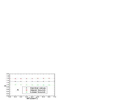
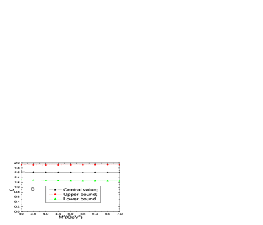
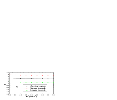
Figure 1: $g_{DD\rho}$(A), $g_{DD_{s}K^{*}}$(B) and $g_{D_{s}D_{s}\phi}$(C) with the Borel parameter $M^{2}$.

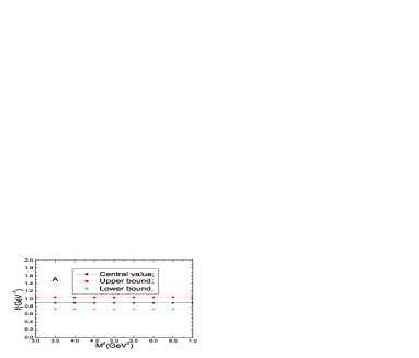
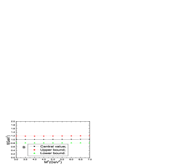
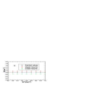
Figure 2: $f_{D^{*}D\rho}$(A), $f_{D^{*}D_{s}K^{*}}$(B) and $f_{D^{*}_{s}D_{s}\phi}$(C) with the Borel parameter $M^{2}$.

4 Conclusion

In this article, we study the vertices $DDV$ and $D^{*}DV$ with the light-cone QCD sum rules. The strong coupling constants $g_{DDV}$ and $f_{D^{*}DV}$ play an important role in understanding the final-state re-scattering effects in the hadronic $B$ decays. They are related to the basic parameters $\beta$ and $\lambda$ in the heavy quark effective Lagrangian, the numerical values are much smaller than the existing estimations based on the assumption of vector mesons dominance. If the predictions from the light-cone QCD sum rules are robust, the final-state re-scattering effects maybe overestimated in the hadronic $B$ decays.

Appendix

The light-cone distribution amplitudes of the $K^{*}$ meson are defined by

$$\langle 0|{\bar{u}}(0)\gamma_{\mu}s(x)|K^{*}(p)\rangle = p_{\mu}f_{K^{*}}m_{K^{*}}\frac{\epsilon\cdot x}{p\cdot x}\int_{0}^{1}due^{-iu\,p\cdot x}\left\{\phi_{\parallel}(u)+\frac{m_{K^{*}}^{2}x^{2}}{16}A(u)\right\}$$

$$+\left[\epsilon_{\mu}-p_{\mu}\frac{\epsilon\cdot x}{p\cdot x}\right]f_{K^{*}}m_{K^{*}}\int_{0}^{1}due^{-iu\,p\cdot x}g_{\perp}^{(v)}(u)$$

$$-\frac{1}{2}x_{\mu}\frac{\epsilon\cdot x}{(p\cdot x)^{2}}f_{K^{*}}m_{K^{*}}^{3}\int_{0}^{1}due^{-iu\,p\cdot x}C(u)\,,$$

$$\langle 0|{\bar{u}}(0)s(x)|{K^{*}}(p)\rangle = \frac{i}{2}\left[f_{K^{*}}^{\perp}-f_{K^{*}}\frac{m_{u}+m_{s}}{m_{K^{*}}}\right]m_{K^{*}}^{2}\epsilon\cdot x\int_{0}^{1}due^{-iu\,p\cdot x}h_{\parallel}^{(s)}(u)\,,$$

$$\langle 0|{\bar{u}}(0)\sigma_{\mu\nu}s(x)|{K^{*}}(p)\rangle = i[\epsilon_{\mu}p_{\nu}-\epsilon_{\nu}p_{\mu}]f_{K^{*}}^{\perp}\int_{0}^{1}due^{-iu\,p\cdot x}\left\{\phi_{\perp}(u)+\frac{m_{K^{*}}^{2}x^{2}}{16}A_{\perp}(u)\right\}$$

$$+i[p_{\mu}x_{\nu}-p_{\nu}x_{\mu}]f_{K^{*}}^{\perp}m_{K^{*}}^{2}\frac{\epsilon\cdot x}{(p\cdot x)^{2}}\int_{0}^{1}due^{-iu\,p\cdot x}B_{\perp}(u)$$

$$+i\frac{1}{2}[\epsilon_{\mu}x_{\nu}-\epsilon_{\nu}x_{\mu}]f_{K^{*}}^{\perp}m_{K^{*}}^{2}\frac{1}{p\cdot x}\int_{0}^{1}due^{-iu\,p\cdot x}C_{\perp}(u)\,,$$

$$\langle 0|{\bar{u}}(0)\gamma_{\mu}\gamma_{5}s(x)|{K^{*}}(p)\rangle = -\frac{1}{4}\left[f_{K^{*}}-f_{K^{*}}^{\perp}\frac{m_{u}+m_{s}}{m_{K^{*}}}\right]m_{K^{*}}\epsilon_{\mu\nu\alpha\beta}\epsilon^{\nu}p^{\alpha}x^{\beta}$$ (31)

$$\int_{0}^{1}due^{-iu\,p\cdot x}g_{\perp}^{(a)}(u)\,.$$

The light-cone distribution amplitudes of the $K^{*}$ meson are parameterized as

$$\phi_{\parallel}(u,\mu) = 6u(1-u)\left\{1+a_{1}^{\parallel}3\xi+a_{2}^{\parallel}\frac{3}{2}(5\xi^{2}-1)\right\}\,,$$

$$\phi_{\perp}(u,\mu) = 6u(1-u)\left\{1+a_{1}^{\perp}3\xi+a_{2}^{\perp}\frac{3}{2}(5\xi^{2}-1)\right\}\,,$$

$$g_{\perp}^{(v)}(u,\mu) = \frac{3}{4}(1+\xi^{2})+a_{1}^{\parallel}\frac{3}{2}\xi^{3}+\left\{\frac{3}{7}a_{2}^{\parallel}+5\zeta_{3}^{\parallel}\right\}(3\xi^{2}-1)$$

$$+\left\{5\kappa_{3}^{\parallel}-\frac{15}{16}\lambda_{3}^{\parallel}+\frac{15}{8}\widetilde{\lambda}_{3}^{\parallel}\right\}\xi(5\xi^{2}-3)$$

$$+\left\{\frac{9}{112}a_{2}^{\parallel}+\frac{15}{32}\omega_{3}^{\parallel}-\frac{15}{64}\widetilde{\omega}_{3}^{\parallel}\right\}(3-30\xi^{2}+35\xi^{4})\,,$$

$$g_{\perp}^{(a)}(u,\mu) = 6u\bar{u}\left\{1+\left(\frac{1}{3}a_{1}^{\parallel}+\frac{20}{9}\kappa_{3}^{\parallel}\right)C_{1}^{\frac{3}{2}}(\xi)+\right.$$

$$\left.\left(\frac{1}{6}a_{2}^{\parallel}+\frac{10}{9}\zeta_{3}^{\parallel}+\frac{5}{12}\omega_{3}^{\parallel}-\frac{5}{24}\widetilde{\omega}_{3}^{\parallel}\right)C_{2}^{\frac{3}{2}}(\xi)+\left(\frac{1}{4}\widetilde{\lambda}_{3}^{\parallel}-\frac{1}{8}\lambda_{3}^{\parallel}\right)C_{3}^{\frac{3}{2}}(\xi)\right\}$$

$$h_{\parallel}^{(s)}(u,\mu) = 6u\bar{u}\left\{1+\left(\frac{a_{1}^{\perp}}{3}+\frac{5}{3}\kappa^{\perp}_{3}\right)C_{1}^{\frac{3}{2}}(\xi)+\left(\frac{a_{2}^{\perp}}{6}+\frac{5}{18}\omega^{\perp}_{3}\right)C_{2}^{\frac{3}{2}}(\xi)-\frac{1}{20}\lambda_{3}^{\perp}C_{3}^{\frac{3}{2}}(\xi)\right\}\,,$$

$$h_{\parallel}^{(t)}(u,\mu) = 3\xi^{2}+\frac{3}{2}a_{1}^{\perp}\xi(3\xi^{2}-1)+\frac{3}{2}a_{2}^{\perp}\xi^{2}(5\xi^{2}-3)+\frac{5}{8}\omega_{3}^{\perp}(3-30\xi^{2}+35\xi^{4})$$

$$+\left(\frac{15}{2}\kappa_{3}^{\perp}-\frac{3}{4}\lambda_{3}^{\perp}\right)\xi(5\xi^{2}-3)\,,$$

$$g_{3}(u,\mu) = 1+\left\{-1-\frac{2}{7}a_{2}^{\parallel}+\frac{40}{3}\zeta_{3}^{\parallel}-\frac{20}{3}\zeta_{4}\right\}C_{2}^{\frac{1}{2}}(\xi)$$

$$+\left\{-\frac{27}{28}a_{2}^{\parallel}+\frac{5}{4}\zeta_{3}^{\parallel}-\frac{15}{16}\widetilde{\omega}_{3}^{\parallel}-\frac{15}{8}\omega_{3}^{\parallel}\right\}C_{4}^{\frac{1}{2}}(\xi)\,,$$

$$h_{3}(u,\mu) = 1+\left\{-1+\frac{3}{7}a_{2}^{\perp}-10(\zeta_{4}^{T}+\widetilde{\zeta}_{4}^{T})\right\}C_{2}^{\frac{1}{2}}(\xi)+\left\{-\frac{3}{7}a_{2}^{\perp}-\frac{5}{4}\omega_{3}^{\perp}\right\}C_{4}^{\frac{1}{2}}(\xi)\,,$$

$$A(u,\mu) = 30u^{2}\bar{u}^{2}\left\{\frac{4}{5}+\frac{4}{105}a_{2}^{\parallel}+\frac{8}{9}\zeta_{3}^{\parallel}+\frac{20}{9}\zeta_{4}\right\}\,,$$

$$A_{\perp}(u,\mu) = 30u^{2}\bar{u}^{2}\left\{\frac{2}{5}+\frac{4}{35}a_{2}^{\perp}+\frac{4}{3}\zeta_{4}^{T}-\frac{8}{3}\widetilde{\zeta}_{4}^{T}\right\}\,,$$

$$C(u,\mu) = g_{3}(u,\mu)+\phi_{\parallel}(u,\mu)-2g_{\perp}^{(v)}(u,\mu)\,,$$

$$B_{\perp}(u,\mu) = h_{\parallel}^{(t)}(u,\mu)-\frac{1}{2}\phi_{\perp}(u,\mu)-\frac{1}{2}h_{3}(u,\mu)\,,$$

$$C_{\perp}(u,\mu) = h_{3}(u,\mu)-\phi_{\perp}(u,\mu)\,,$$ (32)

where $\xi=2u-1$, and $C_{2}^{\frac{1}{2}}(\xi)$, $C_{4}^{\frac{1}{2}}(\xi)$, $C_{1}^{\frac{3}{2}}(\xi)$, $C_{2}^{\frac{3}{2}}(\xi)$, $C_{3}^{\frac{3}{2}}(\xi)$ are Gegenbauer polynomials. The corresponding light-cone distribution amplitudes for the $\rho$ and $\phi$ mesons can be obtained with a simple replacement of the nonperturbative parameters.

References

[1] P. Colangelo, G. Nardulli, N. Paver, Riazuddin, Z. Phys. C45 (1990)
575; M. Ciuchini, E. Franco, G. Martinelli, L. Silvestrini, Nucl. Phys.
B501 (1997) 271; M. Ciuchini, R. Contino, E. Franco, G.
Martinelli, L. Silvestrini, Nucl. Phys. B512 (1998) 3; Y. S.
Dai, D. S. Du, X. Q. Li, Z. T. Wei and B. S. Zou, Phys. Rev. D60 (1999) 014014; C. Isola, M. Ladisa, G. Nardulli, T. N. Pham, P.
Santorelli, Phys. Rev. D64 (2001) 014029; Phys. Rev. D65
(2002) 094005; M. Ablikim, D. S. Du and M. Z. Yang, Phys. Lett. B536 (2002)
34; P. Colangelo, F. De Fazio, Phys. Lett. B542 (2002)
71; M. Ladisa, V. Laporta, G. Nardulli, P. Santorelli, Phys. Rev. D70 (2004)
114025; X. Liu, B. Zhang, S. L. Zhu,
Phys. Lett. B645 (2007) 185; C. Meng, K. T. Chao,
hep-ph/0703205.
[2] H. Y. Cheng, C. K. Chua, A. Soni,
Phys. Rev. D71 (2005) 014030.
[3] R. Casalbuoni, A. Deandrea, N. Di Bartolomeo, R. Gatto, F. Feruglio,
G. Nardulli, Phys. Rept. 281 (1997) 145.
[4] M. Bando, T. Kugo and K.Yamawaki, Nucl. Phys. B259 (1985) 493; Phys. Rept. 164 (1988)
217.
[5]
I. I. Balitsky, V. M. Braun and A. V. Kolesnichenko, Nucl. Phys.
B312 (1989) 509; V. L. Chernyak and I. R. Zhitnitsky, Nucl.
Phys. B345 (1990) 137; V. L. Chernyak and A. R. Zhitnitsky,
Phys. Rept. 112 (1984) 173; V. M. Braun and I. E. Filyanov, Z.
Phys. C44 (1989) 157; V. M. Braun and I. E. Filyanov, Z.
Phys. C48 (1990) 239.
[6]
V. M. Braun, hep-ph/9801222; P. Colangelo and A. Khodjamirian,
hep-ph/0010175.
[7] Z. H. Li, T. Huang, J. Z. Sun, Z. H. Dai, Phys. Rev.
D65 (2002) 076005.
[8] M. A. Shifman, A. I. Vainshtein and V. I. Zakharov,
Nucl. Phys. B147 (1979) 385, 448; L. J. Reinders, H.
Rubinstein and S. Yazaki, Phys. Rept. 127 (1985) 1; S.
Narison, QCD Spectral Sum Rules, World Scientific Lecture Notes in
Physics 26 (1989) 1.
[9]
V. M. Belyaev, V. M. Braun, A. Khodjamirian and R. Rückl, Phys.
Rev. D51 (1995) 6177.
[10] P. Ball, V. M. Braun, Nucl. Phys. B543 (1999) 201;
P. Ball, V. M. Braun,
hep-ph/9808229; P. Ball, V. M. Braun, Phys. Rev. D54 (1996)
2182; P. Ball, V. M. Braun, Y. Koike, K. Tanaka, Nucl. Phys. B529 (1998) 323; P. Ball, G. W. Jones, R. Zwicky, Phys. Rev. D75 (2007) 054004; P. Ball, G. W. Jones, JHEP 0703 (2007)
069.
[11]L. Li, Z. G. Wang, T. Huang, Phys. Rev. D70 (2004)
074006; B. Melic, Phys. Lett. B591 (2004) 91.
[12] Z. G. Wang, J. Phys. G34 (2007) 753.
[13] Z. G. Wang, J. Phys. G34 (2007) 493.
[14] Z. G. Wang, Phys. Rev. D75 (2007) 034013.
[15] H. Kim, S. H. Lee and M. Oka, Prog. Theor. Phys. 109 (2003)
371.
[16]Z. G. Wang, W. M. Yang, S. L. Wan, Nucl. Phys. A744 (2004)
156; J. Bordes, J. Penarrocha, K. Schilcher, JHEP 0511 (2005)
014; L. Lellouch, C. J. David, Phys. Rev. D64 (2001) 094501.
[17] M. Artuso et al, Phys. Rev. Lett. 95 (2005)
251801; G. Bonvicini et al, Phys. Rev. D70 (2004) 112004; T.
K. Pedlar, et al, arXiv:0704.0437[hep-ex].
[18] K. C. Bowler et al, Nucl. Phys. B619 (2001) 507.
[19] A. Hayashigaki, K. Terasaki, hep-ph/0411285.
[20] C. Isola, M. Ladisa, G. Nardulli, P. Santorelli, Phys. Rev. D68 (2003) 114001.
[21] R. Casalbuoni, A. Deandrea, N. Di Bartolomeo, R. Gatto,
F. Feruglio, G. Nardulli, Phys. Lett. B292 (1992) 371; R.
Casalbuoni, A. Deandrea, N. Di Bartolomeo, R. Gatto, F. Feruglio, G.
Nardulli, Phys. Lett. B299 (1993) 139; R. Casalbuoni, A.
Deandrea, N. Di Bartolomeo, R. Gatto, G. Nardulli, Phys. Lett. B312 (1993) 315.
[22] A. Khodjamirian, R. Ruckl, S. Weinzierl,
O.Yakovlev, Phys. Lett. B457 (1999) 245.
[23] D. Becirevic, J. Charles, A. LeYaouanc, L. Oliver,
O. Pene, J. C. Raynal, JHEP 0301 (2003) 009.
[24] A. Khodjamirian, AIP Conf. Proc. 602 (2001)
194.