Electronic structure of the molecule based magnet Cu PM(NO₃)₂ (H₂O)₂

Abstract

We present density functional calculations on the molecule based $S=\frac{1}{2}$ antiferromagnetic chain compound Cu PM(NO₃)₂ (H₂O)₂; PM = pyrimidine. The properties of the ferro- and antiferromagnetic state are investigated at the level of the local density approximation and with the hybrid functional B3LYP. Spin density maps illustrate the exchange path via the pyrimidine molecule which mediates the magnetism in the one-dimensional chain. The computed exchange coupling is antiferromagnetic and in reasonable agreement with the experiment. It is suggested that the antiferromagnetic coupling is due to the possibility of stronger delocalization of the charges on the nitrogen atoms, compared to the ferromagnetic case. In addition, computed isotropic and anisotropic hyperfine interaction parameters are compared with recent NMR experiments.

I Introduction

Molecule based magnetic materials have been the subject of intense research, with the target of designing new magnetic materialsKahnBuch . For example, novel quantum phenomena such as quantum tunneling of magnetization open up possible future applications in quantum computing and data storage Friedman1996 ; Thomas1996 ; Barbara1999 ; Gatteschi2003 . Other interesting research directions are spin state transitions Guetlich , or tuning of the magnetic coupling and the design of ferromagnets (see, e.g. Verdaguer2001 ; pilawa1999 ). This has led to an interdisciplinary effort in physics and chemistry, and by experimentalists and theoreticians.

Supramolecular complexes of transition metals with organic ligands can also be used to synthesize low-dimensional magnets. The organic ligands constitute magnetic superexchange pathways with a strength of the order of 1 to 100 Kelvin. Since pyrimidine and similar heterocycles (pyrazine, pyridine) are often found as magnetic exchange mediating molecules in metal-organic magnets (e.g. Kreitlow ; Clerac2002 ; Hammar1999 ), it is important to study in detail the electronic structure and magnetic exchange mechanism.

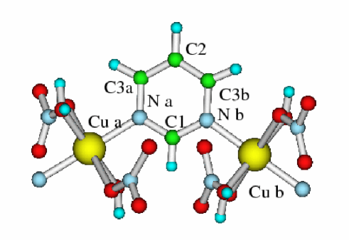
Figure 1: A cutout of the one dimensional chain of Cu PM(NO₃)₂ (H₂O)₂.

Cu PM(NO₃)₂ (H₂O)₂ is a molecule based magnet which can be considered as a one dimensional spin chain (see figure 1). This complex was synthesized a few years ago Ishida1997 . It has been studied by magnetic susceptibility, specific heat and electron spin resonance measurements Feyerherm2000 . More recently, high field magnetization studies anja2003prb and ¹³C NMR measurements were performed anja2003poly ; anja2005prl . It can be theoretically described as a $S=\frac{1}{2}$ antiferromagnetic Heisenberg chain with an exchange coupling of $J$=36 K Feyerherm2000 ; Yasui2001 ; anja2003prb , and with an additional Dzyaloshinskii-Moriya interaction and a staggered g-tensor Oshikawa1997 ; anja2005prl . This model had also been used for other one-dimensional spin chain systems such as copper benzoate Dender1997 ; Asano2000 or CuCl₂ $\cdot$ 2(dimethylsulfoxide) Kenzelmann2004 .

Earlier, a molecular orbital study based on the extended Hückel approach had been performed to gain an insight in the origin of the magnetic interaction and to study the magnetic pathway Mohri1999 . The extended Hückel method can be viewed as a first step in the hierarchy of ab initio calculations.

In this article, we present a density functional study of this system, in order to obtain results based on first principles calculations, without using experimental data (apart from the positions of the nuclei). The target is to get an understanding of the charge- and spin distribution by an analysis of spin density maps and a calculation of the individual magnetic moments. By computing the energy difference between ferro- and antiferromagnet, the exchange coupling $J$ can be extracted. In addition, NMR parameters such as the isotropic and anisotropic hyperfine interaction parameters are computed and compared with recent experimental values. The aim is to get an understanding of the counter-intuitive experimental result, that an atom with a relatively large distance to the magnetic ion has a larger isotropic shift than an atom closer to this magnetic ion. The density functional approach allows to obtain all these properties on equal footing.

II Method

The calculations were done with the code CRYSTAL2003 Manual03 . This code employs a local basis set made of Gaussian type functions. For Cu, a $[5s4p2d]$ basis set KCuF3 , for O a $[4s3p]$ basis setDovesiChemPhys1991 (with outermost $sp$ exponents of 0.5 and 0.191), for N as $[3s2p1d]$, for C a $[3s2p1d]$, and for H a $[2s1p]$ basis set was chosen; the latter three basis sets were as in Feyerherm2004 . Full potential, all electron density functional calculations with the local density approximation (LDA) and with the hybrid functional B3LYP were performed. These calculations were done for the ferro- and antiferromagnetic state, where the resultant solution of the Kohn-Sham equations is an eigenstate of $S_{z}$, but not of $\bf S^{2}$. The energy difference was therefore fitted to an Ising model, in order to estimate the exchange coupling $J$. From the computed spin density, the isotropic and the anisotropic hyperfine coupling parameters are extracted. The charge and spin of the individual atoms are obtained via the Mulliken population analysis.

III Results

III.1 Charge and spin densities

In table 1, the Mulliken populations of the ferromagnetic solution are displayed. Copper carries a charge of $\sim$ +1.6, i.e. less than a formal charge of +2. Consequently, the total spin is $\sim$ 0.7, which indicates that the spin is delocalized to the neighboring atoms. Concerning the pyrimidine ring, we notice that the nitrogen atoms are negatively (-0.7) and the carbon atoms positively charged, so that the ring as a whole is positively charged (0.3). The charge on NO₃ is $\sim$ -0.9, and H₂O is approximatively neutral. The largest spin on the pyrimidine ring ($\sim$ 0.1) is located on the nitrogen atoms of the pyrimidine ring which are neighbors to the copper ions. Comparing LDA and B3LYP, we note that the LDA solution gives a slightly more delocalized picture. This is consistent with previous findings, e.g. MartinIllas1997 ; moreira ; harald1 ; harald2 where it was shown that LDA overemphasizes delocalization. The spin in the pyrimidine ring is alternating up and down, consistent with the idea of a spin polarization mechanism. Looking at the individual sites, for C1 and C3 essentially the $p$-orbitals carry the spin, whereas for C2 the C $s$ orbital carries a little more spin.

In table 2, the corresponding results for the spin of the antiferromagnetic solution are displayed. The charges are virtually identical to the charges of the ferromagnetic solution and thus not displayed. The total spin is similar to the ferromagnetic case for the copper atom, and for the nitrogen atoms of the pyrimidine ring (apart from the sign, obviously). The spin is zero for the C1 and C2 sites due to the symmetry. For the C3 site, there is in the case of the LDA a very small spin, parallel to the spin of the nearest copper, in contrast to the ferromagnetic case, where the spin is antiparallel.

Table 1: Results from the Mulliken population analysis for the ferromagnetic solution.

	B3LYP		LDA
atom	charge	spin	charge	spin
Cu	1.6	0.7	1.5	0.6
N	-0.7	0.09	-0.6	0.128
C1	0.7	-0.01	0.7	- 0.006
H bonded to C1	0.03	0.003	0.04	0.003
C2	0.09	0.01	0.10	0.02
H bonded to C2	0.02	0.002	0.03	0.003
C3	0.4	-0.009	0.4	-0.005
H bonded to C3	0.000	0.002	-0.001	0.003
$\Rightarrow$ Pyrimidine	0.3	0.2	0.4	0.3
NO3	-0.9	0	-0.8	0.01
H2O	-0.1	0.05	-0.1	0.06

Table 2: Results from the Mulliken population analysis for the antiferromagnetic solution.

	B3LYP	LDA
atom	spin	spin
Cu a,b	$\pm$ 0.7	$\pm$ 0.6
N a,b	$\pm$ 0.08	$\pm$ 0.10
C1	0.000	0.000
H bonded to C1	0.000	0.000
C2	0.000	0.000
H bonded to C2	0.000	0.000
C3 a,b	0.000	$\pm$ 0.003
H bonded to C3a,b	$\pm$ 0.001	$\pm$ 0.002
$\Rightarrow$ Pyrimidine	0	0
NO3 bonded to Cu a,b	0	$\pm$ 0.01
H2O attached to Cu a,b	$\pm$ 0.05	$\pm$ 0.06

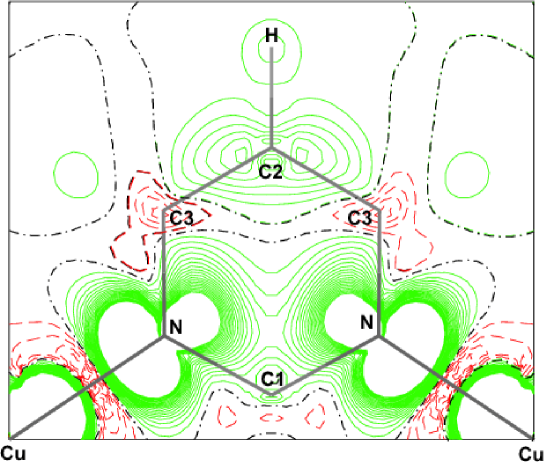
Figure 2: Spin density of the ferromagnetic solution, in atomic units (1/a${}_{0}^{3}$, with the Bohr radius a₀), at the B3LYP level. Full contour lines represent positive spin density, dashed lines negative spin density, and the dashed-dotted line represent zero spin density. The lines have a distance of 0.00025/a${}_{0}^{3}$.

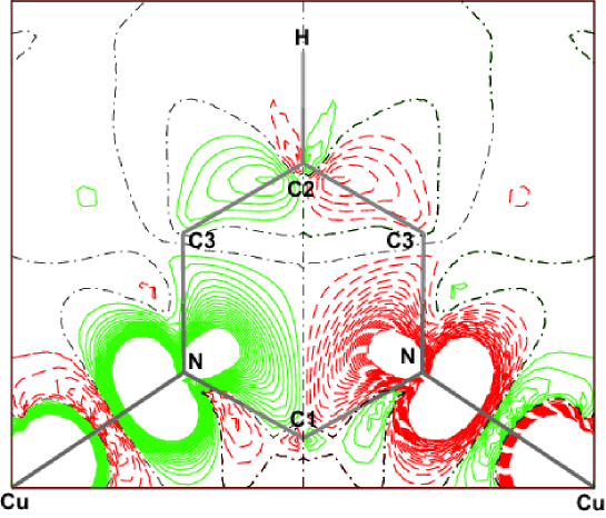
Figure 3: Spin density of the antiferromagnetic solution, in atomic units (1/a${}_{0}^{3}$), at the B3LYP level. Full contour lines represent positive spin density, dashed lines negative spin density, and the dashed-dotted line represent zero spin density. The lines have a distance of 0.00025/a${}_{0}^{3}$.

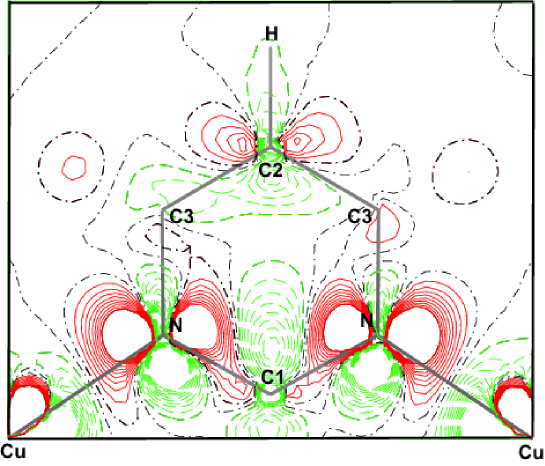
Figure 4: The difference of the charge density of the ferromagnetic and the antiferromagnetic solution, in atomic units ($|e|$/a${}_{0}^{3}$), at the B3LYP level. Full contour lines represent regions where the density is higher in the ferromagnetic case, dashed lines represent regions where the density is higher in the antiferromagnetic case. The dashed-dotted line corresponds to zero. The lines have a distance of 0.00001$|e|$/a${}_{0}^{3}$.

These results are visualized in the spin density plots for ferromagnetic (figure 2) and antiferromagnetic (figure 3) spin density, at the B3LYP level. It is obvious that neighboring copper and nitrogen atoms always have parallel spin. In the ferromagnetic case, the adjacent carbon atoms (C3) have a spin which is antiparallel to the nitrogen atoms: antiparallel spin between neighboring atoms reduces the Pauli repulsion. This allows a more diffuse charge distribution and thus reduces the energy. Finally, the carbon atom C2 has again an antiparallel spin with respect to the neighboring carbon atoms (C3), in order to reduce the Pauli repulsion. In the antiferromagnetic case, the arguments hold similarly, but additionally, the cancellation of negative and positive spin density must be taken into account which results in a total spin of zero or nearly zero at the carbon sites.

Comparing the ferro- and antiferromagnetic solutions, the antiferromagnetic spin density allows the charge densities of the two nitrogen atoms to stronger interpenetrate in the center of the ring, which is suppressed in the ferromagnetic case because of the Pauli principle. This is illustrated in figure 4 where it is shown that the charge density in the ring is slightly higher for the antiferromagnetic solution. As a whole, this results in a stronger delocalization of the nitrogen charge in the antiferromagnetic case and thus reduces the total energy, which supports the antiferromagnetic coupling observed experimentally.

III.2 Magnetic hyperfine interaction

Table 3: Fermi contact coupling, at the level of LDA and B3LYP, versus the experimental value, in 1/a${}_{0}^{3}$, with the Bohr radius a₀.

site	LDA	B3LYP	experiment anja2005prl
C1	0.008	0.003	0.0045
C2	0.008	0.007	0.034
C3	0.001	-0.0006	-0.006

From the spin densities, it is possible to compute the isotropic Fermi contact and the dipolar contribution to the anisotropic hyperfine coupling. The isotropic part is given by the spin density at the carbon nuclei, and can be compared with the values obtained from ¹³C NMR anja2005prl . As a magnetic field is applied in the experiment, we therefore have to use the Fermi couplings obtained with the ferromagnetic solution. The data are displayed in Table 3. It should be mentioned that computing Fermi contact couplings accurately is a notorious problem already for molecules KauppBuch . This is even more difficult here, as the spin density must be evaluated at the position of atoms which are far away from the magnetic copper ions, i.e. transferred hyperfine fields. The B3LYP approach reproduces the signs of the spin densities at the different atoms properly: the spin density at the carbon nucleus is positive for C1 and C2, and negative for C3. Note that the total spin is negative for C1, whereas the spin density at the nucleus is positive and even in rough quantitative agreement with the experimental value. For the C3 site, we find a small negative spin density at the nucleus, in qualitative agreement with the experiment. Finally, for the C2 site, a positive Fermi contact coupling is found which is the largest of the values computed. Again, this is in qualitative agreement with the experiment. Note that the value is largest at this site which has the largest distance to the copper atoms; one might rather expect to find larger Fermi couplings for atoms with shorter distances. From the spin density plots, we find an interpretation and explanation: first, in the pyrimidine ring, neighboring atoms have antiparallel spin, so that we find alternating up and down spin. As the nitrogen spin is very large, the C1 atom has a relatively small spin density because the negative C1 spin is partially compensated by the positive nitrogen spin which is spatially extended towards the C1 site. In addition, the carbon spin resides essentially in the $p$ orbital which has a node at the nucleus and thus does not contribute to the spin density. In contrast, at the C2 site, a spin parallel to the nitrogen spin is obtained and mediated via both adjacent carbon atoms. The carbon $s$ orbital, which has a non-vanishing spin density at the carbon nucleus, contributes slightly more to the spin for the C2 site. Thus, we find a relatively large isotropic hyperfine coupling although this atom has the largest distance to the copper atoms carrying the majority of the spin. Finally, the carbon atom at C3 has relatively small spin with opposite sign; here again the negative spin of the carbon is compensated by the neighboring positive spin of the nitrogen and C2.

It becomes also apparent that B3LYP fits better to the experimental values than LDA does; the different sign for the site C3 can only be confirmed at the B3LYP level.

In a next step, the components of the anisotropic hyperfine tensor are computed. These are computed as the expectation value of the operator

$$T_{ijA}=\sum_{\mu,\nu}\sum_{\vec{g}}P_{\mu,\nu,\vec{g}}^{spin}\int\varphi_{\mu}(\vec{r})\left(\frac{\vec{r}_{A}^{2}\delta_{ij}-3\vec{r}_{A_{i}}\vec{r}_{A_{j}}}{r_{A}^{5}}\right)\varphi_{\nu,\vec{g}}(\vec{r})d^{3}r$$

where $\varphi_{\nu}$ are the Gaussian type basis functions, $P_{\mu,\nu,\vec{g}}^{spin}$ is the density matrix for the difference of up and down spin, $\vec{g}$ are lattice vectors, and $\vec{r}_{A}$ is the distance $\vec{r}$-$\vec{A}$, with $\vec{A}$ being the position of the nucleus for which the anisotropic dipole hyperfine tensor is computed. The results of these calculations are presented in table 4. A comparison is made with the results from a point lattice dipole moment where 90 % of the spin was allocated at the copper site, and 5 % at each of the two nitrogen atoms of the pyrimidine ring. This was found to be the best fit to the measured NMR data anja2005prl . Such a spin distribution is similar to the one obtained in the present work by a first principles density functional calculation. Comparing the dipolar tensors, we find a reasonable agreement between the three approaches used (point dipolar model, LDA, B3LYP). This is also demonstrated in figure 5, where the computed anisotropic hyperfine interaction tensor was used, together with experimentally determined NMR chemical shift and isotropic hyperfine interaction. It can be seen that the data is reasonably well fitted, but also the dependence on the functional becomes obvious; and B3LYP fits the data better.

It should be mentioned that the results for the hyperfine interaction were obtained with the basis set as described in section II. As this property depends on the spin density of the nucleus, additional calculations were performed with e.g. a much larger set of tighter carbon $s$ and $p$ basis functions to describe the electron density in the region of the nucleus better. We found that the results were essentially stable with respect to various basis sets employed.

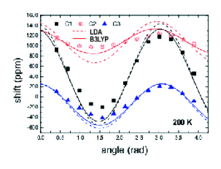
Figure 5: A comparison of experimental data for the C1 (squares), C2 (circles) and C3 (triangles) sites and a fit using experimental values for NMR chemical shift and isotropic shift, and computed values (LDA, B3LYP) for the anisotropic shift.

III.3 Magnetic exchange coupling

The magnetic exchange coupling is usually obtained by computing the energy difference between two magnetic states, and fitting it to a model Hamiltonian. This means that the energies of at least two magnetic states have to be computed, in order to extract $J$ from the energy difference.

In the case of molecules, the energy can be computed with accurate wave function based methods such as the multi-reference configuration interaction scheme, multi-reference perturbation theory and related methods Fink1 ; Fink2 ; Graaf2001 ; Calzado2000 ; MoreiraKNiF ; harald2 . The advantage is that the correlation treatment is well controlled, and by taking into account more and more determinants, a fairly accurate calculation of the exchange coupling is possible. In addition, the wave function can be constructed as an eigenstate of $\bf{S^{2}}$. On the other hand, such calculations are very demanding in terms of memory requirement, and are usually limited to few magnetic centers (two in most cases). In addition, it may be necessary to truncate large molecules and create some embedding. An alternative is to use methods such as unrestricted Hartree-Fock theory or density functional theory and apply them to molecules.

In the case of solids, a wave-function based treatment of the periodic solid is usually prohibitive. Thus, a possible way is to use schemes such as Hartree-Fock theory or density functional theory which can be applied to solids. This approach can be performed whenever the unit cell is not too large.

The main downside of Hartree-Fock theory is that it gives a too localized picture and usually strongly underestimates the exchange coupling, often by a factor of 3: e.g. for NiO and MnO Towler1994 , KXF₃ (X=Mn,Fe,Co,Ni) Ricart1995 ; Dovesi1997 or KCuF₃, K₂CuF₄ and Sr₂CuO₂Cl₂ KCuF3 ; Moreira2004IJQC .

The local density approximation, on the other hand, strongly overestimates the exchange coupling, because the charges are too delocalized and thus exchange integrals are too large. This overestimation is often as large as a factor of 5: e.g. for NiO moreira , KCuF₃, K₂CuF₄ and Sr₂CuO₂Cl₂ Moreira2004IJQC . Gradient corrections only slightly change this and again, an overestimation was observed, e.g. Kortus2001 ; harald1 . The situation is more difficult in systems where various couplings are important, e.g. Park2004 . The hybrid functional B3LYP was initially designed for molecules, but has become very popular in solid state physics because the band gaps obtained are in surprisingly good agreement with experiment Joe . It interpolates between Hartree-Fock theory and density functional theory, and is now also frequently used for the calculation of superexchange coupling constants, where it overestimates exchange couplings by a factor of the order of $\lesssim$ 2, e.g. NiO moreira , KCuF₃, K₂CuF₄ and Sr₂CuO₂Cl₂ Moreira2004IJQC ; Feng2004 , or La₂CuO₄, La₂NiO₄, KNiF₃, NiF₂, MnF₂, KMnF₃ Feng2004 , or FeCl₂(PM)₂ and NiCl₂(PM)₂ Kreitlow . Finally, it should be mentioned that there are exceptions to these simple rules of thumb, especially in cases where the two magnetic centers and the bridging atom(s) show a strong deviation from an 180^∘ angle and approach 90^∘, i.e. strongly deviate from being on a straight line, e.g. $J_{1}$ in MnF₂ and NiF₂ Moreira2000p7816 ; Feng2004 , or the ferric wheel-like molecule as in harald1 ; harald2 . In these cases, the coupling is small according to the Goodenough-Kanamori rules KahnBuch and a calculation becomes more difficult.

A broken symmetry approach and subsequent spin projection was suggested as a way of obtaining eigenstates of $\bf{S^{2}}$ in the case of molecules Noodleman1981 . Further suggestions to deal with magnetic states were the spin-restricted open shell Kohn-Sham (ROKS) ROKS and the spin-restricted ensemble-referenced Kohn-Sham method (REKS) REKS . There is an ongoing discussion about the validity of the various approaches, see e.g. Caballol1997 ; Illas2000 ; Illas2004 ; IllasTCA2006 . Very recently, Ruiz et al suggested that one problem was that the self interaction error was taken into account twice when spin projection was applied together with a self interaction correction Ruiz2005JCP . This was however challenged Adamoetal2006 , and it was argued that there was no firm theoretical basis for this argument.

In the case of solids, the only computationally feasible way is to use a broken symmetry approach (without spin-projection). The solution of the Hartree-Fock or Kohn-Sham equations is thus in general not an eigenstate of $\bf{S^{2}}$, but only of $S_{z}$, and the spatial symmetry is broken. The data can be fitted to an Ising model, and should rather not be fitted to the Heisenberg model. This approach was actually recommended as a ’simple yet elegant way out of this problem’ MoreiraIllas2006PCCP (where ’this problem’ refers to the problem described in the preceding paragraph).

A different way of treating solids would be to use some embedded cluster scheme which again allows to apply the same quantum chemical methods as in the molecular case. However, the truncation is not obvious and poses again an approximation.

The issue of using configuration interaction or spin-projection was also discussed in the context of quantum dots: systems with few electrons are considered, and a model Hamiltonian is chosen where parameters such as the effective mass and the dielectric constant are extracted from the experiment. This allows to construct the wave function on the level of configuration interaction and as an eigenstate of $\bf{S^{2}}$, and the importance of doing so was discussed for this class of systems, e.g. Ellenberger ; Melnikov ; Yannouleas ; ReimannRMP . However, these systems are very different from the one considered here: in the present work, localized spins are considered, and the orbital occupancy of the magnetic ions is essentially determined by the crystal field. The ground state is thus often better described by a single reference wave function, compared to the case of molecules, where often a multi-reference wave function is necessary. In the case of quantum dots, the situation is different: besides examples where the local density approximation works surprisingly well, e.g. Reimann2000 , there are other situations where a description by a single determinant may be poor, e.g. in the case of large magnetic fields or in double dots Melnikov , and it becomes necessary to use configuration interaction schemes.

As we are interested in a uniform description of properties such as the spin and charge density and NMR parameters, we therefore evaluated these properties and the exchange coupling at the same level of theory. The strength of the magnetic exchange interaction $J$ is thus computed by fitting the energy difference between ferro- and antiferromagnet to an Ising model: $H=\sum_{i}JS_{i}S_{i+1}$. The data obtained for $J$ are a prerequisite required if one was interested in quantum tunneling; the calculation of the anisotropy would be a further step (which requires spin-orbit coupling).

There are two copper atoms per cell, and thus two couplings of the size $J$. The energy difference between ferro- and antiferromagnet is thus $\Delta E=E_{FM}-E_{AF}=2zS^{2}J$ where $z$ is the number of couplings per cell, i.e. 2 in this case. For $S=\frac{1}{2}$, we obtain thus $\Delta E=J$. The computed couplings are displayed in table 5. At the B3LYP level, a value of 76 K is obtained, at the LDA level a value of 603 K. The B3LYP value is by a factor of 2 too large, compared to the experimental value of $J$=36 K Feyerherm2000 ; Yasui2001 ; anja2003prb . The LDA value is even larger, because the LDA density is much more delocalized. Such overestimations of computed exchange couplings are typical for the functionals employed, as was mentioned above. The B3LYP density is more localized and thus a value closer to the experiment is obtained. These findings are consistent with the Mulliken charges in tables 1 and 2, where a more covalent picture was obtained with the LDA.

Table 4: Dipolar tensors at the carbon sites: the first value corresponds to the level of a localized dipole model, the second to LDA and the third one to B3LYP, in 1/a${}_{0}^{3}$. The components are given using a cartesian coordinate system.

C1

$$\left(\begin{array}[]{ccc}0.01;0.007;0.006&0;0;0&0.022;0.036;0.033\\ 0;0;0&-0.011;-0.007;-0.005&0;0;0\\ 0.022;0.036;0.033&0;0;0&0.0004;-0.0006;-0.001\end{array}\right)$$

C2

$$\left(\begin{array}[]{ccc}0.0005;0.0005;0.001&0;0;0&0.0007;0.01;0.003\\ 0;0;0&0.002;0.0002;-0.001&0;0;0\\ 0.0007;0.01;0.003&0;0;0&0.002;-0.0007;0.00001\end{array}\right)$$

C3

$$\left(\begin{array}[]{ccc}-0.004;-0.01;-0.008&\pm 0.004;\pm 0.007;\pm 0.005&0.002;0.01;0.01\\ \pm 0.004;\pm 0.007;\pm 0.005&0.01;0.02;0.02&\pm 0.002;\pm 0.006;\pm 0.004\\ 0.002;0.01;0.01&\pm 0.002;\pm 0.006;\pm 0.004&-0.006;-0.01;-0.01\end{array}\right)$$

Table 5: Energy difference between ferromagnetic and antiferromagnetic solution and exchange coupling $J$.

functional	$\Delta E$ ($E_{h}$)	$J$ ($E_{h}$)	$J$ (eV)	$J$ (K)
B3LYP	0.00024	0.00024	0.0065	76
LDA	0.0019	0.0019	0.052	603

IV Conclusion

Density functional calculations on the molecule based magnet Cu PM(NO₃)₂ (H₂O)₂ were performed, using the local density approximation and the hybrid functional B3LYP. The exchange path via the pyrimidine ring was analyzed with spin density plots and with a Mulliken spin population. The calculations prove a spin transfer from the Cu atom to the adjacent nitrogen atoms as had been deduced from the NMR experiments. The spin of the nitrogen atoms in the pyrimidine ring is parallel to the copper spin in all cases. In the ferromagnetic case, the spin on the pyrimidine ring is alternating. The carbon atoms C1 and C3 have a spin essentially in the $p$ orbitals, and on the C2 site also a slightly larger spin is found in the carbon $s$ orbital. In the antiferromagnetic case, the spin is virtually zero on all the carbon atoms.

In the case of the antiferromagnet, the charges of the two nitrogen atoms of the pyrimidine ring can stronger interpenetrate. This delocalization reduces the energy and explains why antiferromagnetism is observed. In addition, the isotropic and anisotropic hyperfine interaction parameters were computed. For the isotropic parameters, a qualitative agreement could be observed with the B3LYP functional. Especially, the experimental result that the isotropic hyperfine coupling is largest at the C2 site, which has the largest distance to the magnetic ion, could be confirmed. It is suggested that this is due to the relatively large contribution to the spin density from the $s$ orbital for the C2 site. In the case of the anisotropic dipolar hyperfine tensor, a good agreement with the experimental data was found for both functionals, where again B3LYP performed better. Finally, the exchange coupling was computed via the energy difference between ferro- and antiferromagnetic state. A reasonable agreement was found at the B3LYP level, whereas the local density approximation results in by far too large values of $J$ due to an enhanced delocalization, which is a well known problem of exchange couplings computed with the LDA.

V Acknowledgement

The authors would like to thank Prof. S. Süllow (Braunschweig) for helpful discussions. This work has been partially supported by the DFG SPP 1137 and contract no. KL 1086/6-1.

References

- (1) O. Kahn, Molecular Magnetism (WILEY-VCH, New York, 1993).
- (2) L. Thomas, F. Lionti, R. Ballou, D. Gatteschi, R. Sessoli and B. Barbara, Natrue 383, 145 (1996).
- (3) J. R. Friedman, M. P. Sarachik, J. Tejada and R. Ziolo, Phys. Rev. Lett. 76, 3830 (1996).
- (4) B. Barbara and L. Gunther, Physics World 12, 35 (1999).
- (5) D. Gatteschi and R. Sessoli, Angew. Chem., Int. Ed. 42, 268 (2003).
- (6) P. Gütlich, A. Hauser and H. Spiering, Angew. Chem. 106, 2109 (1994).
- (7) M. Verdaguer, Polyhedron 20, 1115 (2001).
- (8) B. Pilawa, Ann. Phys. (Leipzig), 8, 191 (1999).
- (9) J. Kreitlow, D. Menzel, A. U. B. Wolter, J. Schoenes, S. Süllow, R. Feyerherm, K. Doll, Phys. Rev. B 72, 134418 (2005).
- (10) R. Clérac, H. Miyasaka, M. Yamashita and C. Coulon, J. Am. Chem. Soc. 124, 12837 (2002).
- (11) P. R. Hammar, M. B. Stone, D. H. Reich, C. Broholm, P. J. Gibson, M. M. Turnbull, C. P. Landee, M. Oshikawa, Phys. Rev. B 59, 1008 (1999).
- (12) T. Ishida, K. Nakayama, M. Nakagawa, W. Sato, Y. Ishikawa, M. Yasui, F. Iwasaki, T. Nogami, Synth. Met. 85, 1655 (1997).
- (13) R. Feyerherm, S. Abens, D. Günther, T. Ishida, M. Meißner, M. Meschke, T. Nogamim, and M. Steiner, J. Phys.: Condensed Matt. 12, 8495 (2000).
- (14) A. U. B. Wolter et al, Phys. Rev. B 68, 220406 (2003).
- (15) A. U. B. Wolter, P. Wzietek, F. J. Litterst, S. Süllow, D. Jérome, R. Feyerherm, H.-H. Klauss, Polyhedron 22, 2273 (2003).
- (16) A. U. B. Wolter, P. Wzietek, S. Süllow, F. J. Litterst, A.Honecker, W. Brenig, R. Feyerherm and H.-H. Klauss, Phys. Rev. Lett. 94, 057204 (2005).
- (17) M. Yasui, Y. Ishikawa, N. Akiyama, T. Ishida, T. Nogami and F. Iwasaki, Acta Cryst. B 57, 288 (2001).
- (18) M. Oshikawa and I. Affleck, Phys. Rev. Lett. 79, 2883 (1997); I. Affleck and M. Oshikawa, Phys. Rev. B 60, 1038 (1999).
- (19) D. C. Dender, P. R. Hammar, D. H. Reich, C. Broholm, and G. Aeppli, Phys. Rev. Lett. 79, 1750 (1997).
- (20) T. Asano, H. Nojiri, Y. Inagaki, J. P. Boucher, T. Sakon, Y. Ajiro, and M. Motokawa, Phys. Rev. Lett. 84, 5880 (2000).
- (21) M. Kenzelmann, Y. Chen, C. Broholm, D. H. Reich, and Y. Qiu, Phys. Rev. Lett. 93, 017204 (2004).
- (22) F. Mohri, K. Yoshizawa, T. Yamabe, T. Ishida, T. Nogami, Mol. Eng. 8, 357 (1999)
- (23) V. R. Saunders, R. Dovesi, C. Roetti, R. Orlando, C. M. Zicovich-Wilson, N. M. Harrison, K. Doll, B. Civalleri, I. J. Bush, Ph. D’Arco, M. Llunell, crystal 2003 User’s Manual, University of Torino, Torino (2003).
- (24) M. D. Towler, R. Dovesi, and V. R. Saunders, Phys. Rev. B 52, 10150 (1995).
- (25) R. Dovesi, C. Roetti, C. Freyria-Fava, M. Prencipe, and V. R. Saunders, Chem. Phys. 156, 11 (1991).
- (26) R. Feyerherm, A. Loose, T. Ishida, T. Nogami, J. Kreitlow, D. Baabe, F. J. Litterst, S. Süllow, H.-H. Klauss, K. Doll, Phys. Rev. B 69, 134427 (2004).
- (27) I. de P. R. Moreira, F. Illas, and R. L. Martin, Phys. Rev. B 65, 155102 (2002).
- (28) R. L. Martin and F. Illas, Phys. Rev. Lett. 79, 1539 (1997).
- (29) H. Nieber, K. Doll and G. Zwicknagl, Eur. Phys. J. B. 44, 209 (2005).
- (30) H. Nieber, K. Doll and G. Zwicknagl, Eur. Phys. J. B. 51, 215 (2006).
- (31) Calculation of NMR and EPR parameters, Editors: M. Kaupp, M. Bühl, V. G. Malkin, Wiley-VCH, Weinheim (2004)
- (32) K. Fink, R. Fink and V. Staemmler, Inorg. Chem. 33, 6219 (1994).
- (33) K. Fink, C. Wang and V. Staemmler, Inorg. Chem. 38, 3847 (1999).
- (34) C. de Graaf, C. Sousa, I. de P. R. Moreira and F. Illas, J. Phys. Chem. A 105, 11371 (2001).
- (35) C. J. Calzado, J. F. Sanz and J. P. Malrieu, J. Chem. Phys. 112, 5158 (2000).
- (36) I. de P. R. Moreira and F. Illas, Phys. Rev. B 55, 4129 (1997).
- (37) M.D. Towler, N.L. Allan, N.M. Harrison, V.R. Saunders, W.C. Mackrodt and E. Aprà, Phys. Rev. B 50, 5041 (1994).
- (38) J. M. Ricart, R. Dovesi, C. Roetti and V. R. Saunders, Phys. Rev. B 52, 2381 (1995); Phys. Rev. B 55, 15942 (1997) (Erratum).
- (39) R. Dovesi, F. Freyria Fava, C. Roetti and V. R. Saunders, Faraday Discuss. 106, 173 (1997).
- (40) I. de P. R. Moreira and R. Dovesi, Int. J. Quant. Chem. 99, 805 (2004).
- (41) J. Kortus, C. S. Hellberg and M. R. Pederson, Phys. Rev. Lett. 86, 3400 (2001).
- (42) K. Park and M. R. Pederson, Phys. Rev. B 70, 054414 (2004).
- (43) J. Muscat, A. Wander, N. M. Harrison, Chem. Phys. Lett. 342, 397 (2001).
- (44) X. Feng and N. M. Harrison, Phys. Rev. B 70, 092402 (2004).
- (45) I. de P. R. Moreira, R. Dovesi, C. Roetti, V. R. Saunders and R. Orlando, Phys. Rev. B 62, 7816 (2000).
- (46) L. Noodleman, J. Chem. Phys. 74, 5737 (1981).
- (47) M. Filatov and S. Shaik, Chem. Phys. Lett. 288, 689 (1998).
- (48) M. Filatov and S. Shaik, Chem. Phys. Lett. 304, 429 (1999).
- (49) R. Caballol, O. Castell, F. Illas, I. de P. R. Moreira, J. P. Malrieu, J. Phys. Chem. A 101, 7860 (1997).
- (50) F. Illas, I. de P. R. Moreira, C. de Graaf and V. Barone, Theor. Chem. Acc. 104, 265 (2000).
- (51) F. Illas, I. de P. R. Moreira, J. M. Bofill and M. Filatov, Phys. Rev. B 70, 132414 (2004).
- (52) F. Illas, I. de P. R. Moreira, J. M. Bofill and M. Filatov, Theor. Chem. Acc. 116, 587 (2006).
- (53) E. Ruiz, S. Alvarez, J. Cano and V. Polo, J. Chem. Phys. 123, 164110 (2005).
- (54) C. Adamo, V. Barone, A. Bencini, R. Broer, M. Filatov, N. M. Harrison, F. Illas, J. P. Malrieu and I. de P. R. Moreira, J. Chem. Phys. 124, 107101 (2006).
- (55) I. de P. R. Moreira and F. Illas, Phys. Chem. Chem. Phys. 8, 1645 (2006).
- (56) C. Ellenberger, T. Ihn, C. Yannouleas, U. Landman, K. Ensslin, D. Driscoll and A. C. Gossard, Phys. Rev. Lett. 96, 126806 (2006).
- (57) D. V. Melnikov and J.-P. Leburton, Phys. Rev. B 73, 155301 (2006).
- (58) C. Yannouleas and U. Landman, Int. J. Quant. Chem. 90, 699 (2002).
- (59) S. M. Reimann and M. Manninen, Rev. Mod. Phys. 74, 1283 (2002).
- (60) S. M. Reimann, M. Koskinen and M. Manninen, Phys. Rev. B 62, 8108 (2000).