A mathematical analysis of the effects of Hebbian learning rules on the dynamics and structure of discrete-time random recurrent neural networks

Abstract

We present a mathematical analysis of the effects of Hebbian learning in random recurrent neural networks, with a generic Hebbian learning rule including passive forgetting and different time scales for neuronal activity and learning dynamics. Previous numerical works have reported that Hebbian learning drives the system from chaos to a steady state through a sequence of bifurcations. Here, we interpret these results mathematically and show that these effects, involving a complex coupling between neuronal dynamics and synaptic graph structure, can be analyzed using Jacobian matrices, which introduce both a structural and a dynamical point of view on the neural network evolution. Furthermore, we show that the sensitivity to a learned pattern is maximal when the largest Lyapunov exponent is close to 0. We discuss how neural networks may take advantage of this regime of high functional interest.

I Introduction

The mathematical study of the effects of synaptic plasticity (or more generally learning) in neural networks is a difficult task because the dynamics of the neurons depends on the synaptic weights network, that itself evolves non trivially under the influence of neuron dynamics. Understanding this mutual coupling (and its effects on the computational efficiency of the neural network) is a key problem in computational neuroscience and necessitates new analytical approaches.
In recent years, the related field of dynamical systems interacting on complex networks has attracted vast interest. Most studies have focused on the influence of network structure on the global dynamics (for a review, see Boccaletti et al. (2006)). In particular, much effort has been devoted to the relationships between node synchronization and the classical statistical quantifiers of complex networks (degree distribution, average clustering index, mean shortest path, motifs, modularity…) Grinstein and Linsker (2005); Nishikawa et al. (2003); Lago-Fernández et al. (200). The core idea was that the impact of network topology on global dynamics might be prominent, so that these structural statistics may be good indicators of global dynamics. This assumption proved however largely wrong and some of the related studies yielded contradictory results Nishikawa et al. (2003); Hong et al. (2002). Actually, synchronization properties cannot be systematically deduced from topology statistics but may be inferred from the spectrum of the network Atay et al. (2006). Most of these studies have considered diffusive coupling between the nodes Hasegawa (2005). In this case, the adjacency matrix has real nonnegative eigenvalues, and global properties, such as stability of the synchronized states Barahona and Pecora (2002) can easily be inferred from its spectral properties (see also Atay. et al. (2006); Volchenkov and Blanchard (2007) and Chung (1997) for a review on mathematically rigorous results). Unfortunately, the coupling between neurons (synaptic weights) in neural networks is rarely diffusive, the corresponding matrix is not symmetric and may contain positive and negative elements. In addition, the synaptic graph structure of a neural network is usually not fixed but evolves with time, which adds another level of complexity. Hence, these results are not directly applicable to neural networks.
Discrete-time random recurrent neural networks (RRNNs) are known to display a rich variety of dynamical behaviors, including fixed points, limit cycle oscillations, quasi periodicity and deterministic chaos Doyon et al. (1993). The effect of hebbian learning in RRNN, including pattern retrieval properties, has been explored numerically by Daucé and some of us Dauce et al. (1998). It was observed that Hebbian learning leads to a systematic reduction of the dynamics complexity (transition from chaos to fixed point by an inverse quasi-periodicity route). This property has been exploited for pattern retrieval. After a suitable learning phase the presentation of a learned pattern induces a bifurcation (e.g. from chaos to a simpler attractor such as a limit cycle). This effect is inherited via learning (it does not exist before learning), is robust to a small amount of noise, and selective (it does not occur for drastically different patterns). These effects were however neither analyzed nor really understood in Dauce et al. (1998). This work was extended to sequence learning and expoited on a robotic platform in Daucé et al. (2002).
More recently, Echo State Networks (ESN) Jaeger and Haas (2004) have been developed, where, as in our case, the network acts as a reservoir of resonant frequencies. However, learning only affects output links in ESN networks, while the weights within the reservoir are kept constant. Tsuda’s chaotic itinerancy is an alternative way for linking different attractors with different inputs Tsuda (2001). In this model, weights are initially fixed in a Hopfield-like manner (and are thus symmetric) and a chaotic dynamics successively explores the different fixed point attractors. In this scheme, each input constitutes an different initial condition that leads to one attractor of the same dynamical system, whereas in Dauce et al. (1998), each (time-constant) input leads to a different dynamical system.
In the current state of the art, there is a relatively large number of models, observations and applications of Hebbian learning effects in neural networks, but considerably less mathematical results. Mathematical analysis is however necessary to classify the many variants of Hebbian learning rules according to the effects they produce. The present paper is one step further towards this aim. Using methods from dynamical systems theory, we analyze the effects of a generic version of Hebbian learning proposed in Hoppensteadt and Izhikevich (1997) on the neural network model numerically studied in Dauce et al. (1998) with spontaneous (i.e. before learning) chaotic dynamics.
We essentially classify the effects into three families:
(i) Topological: the structure of the synaptic weight network evolves, implying prominent (e.g. cooperative) effects on the dynamics.
(ii) Dynamical: the dynamical complexity (measured e.g. by the maximal Lyapunov exponent or the Kolmogorov-Sinai entropy) reduces during Hebbian learning. This effect is mathematically analyzed and interpreted. Especially, we provide a rigorous upper bound on the maximal Lyapunov exponent and identify two major causes for this reduction: the decay of the norm of the synaptic weight matrix and the saturation of neurons.
(iii) Functional: Focusing on the network response to a learned pattern, we show that there is a learning stage at which the response is maximal, in the sense that it generates a drastic change of the neuronal dynamics (i.e. a bifurcation). This stage precisely corresponds to vanishing of the maximal Lyapunov exponent.
Some of these results may appear neither “new” nor “surprising” for the neural networks community. For example, (ii) and (iii) have already been reported in Dauce et al. (1998). However, the results were mainly numerical while the present paper proposes a mathematical framework and formal tools to analyze them. Moreover, a direct consequence of (iii) is that the response of the neural network to a learned pattern is maximal at the “edge of chaos” (where the maximal Lyapunov exponent vanishes).
The claim that the neural network response is maximal close to a bifurcation is common in the neural network community Langton (1990). Similarly, Hoppensteadt and Izhikevich (1997) already pointed out the necessity for some neurons to lie close to a bifurcation point in order to have relevant computational capacities. As a matter of fact, an analysis of the effects of a Hopfield-Hebb rule was performed in this book with neurons close to codimension one fixed-point bifurcations.
We go a step further in the present paper and show that a similar conclusion holds for a neural network in a chaotic regime. Conceptually, the analysis of Hoppensteadt and Izhikevich (1997) could be extended to chaotic systems Cessac and Samuelides (2007). However, the analytic treatment of the chaotic case is really challenging. Hence, bifurcation analysis of fixed points (or periodic orbits) uses a linear analysis via Jacobian matrices, which is usually considered non-applicable to chaotic systems where nonlinear effects and initial conditions sensitivity are prominent. Nevertheless, recent results by Ruelle Ruelle (1999) on linear response theory, formally extended to chaotic neural networks Cessac and Sepulchre (2006, 2007), show that a linear analysis is indeed possible if one uses an average of the Jacobian matrix along its chaotic trajectory. The associated linear response operator provides a deep insight into the links between topology and dynamics in chaotic neural networks. Incidentally, it shows that the relevant matrix is not the weight matrix (as would be expected), but the linear response matrix, which reduces, in the present context, to the ergodic average of the Jacobian matrix along its trajectory .
Though the main results in this paper are mathematical, we also use some numerical simulations. They were necessary because mathematical results are obtained using a limit where time goes to infinity, which is not operational in numerical situations. Moreover, the central rigorous results we obtain provide upper bounds, whose quality had to be checked numerically.
The paper is organized as follows. We first present the model and the generic framework for neuronal dynamics and learning rules in section II. The following sections are devoted to the analysis of the model. In section III, we present analytical results explaining the evolution of dynamics during learning using mathematical tools from dynamical systems and graph theory. These analytical results are confirmed by extensive numerical simulations. Section IV focuses on functional effects related to network sensitivity to the learned pattern. We finally discuss our results in the last section (V).

II General framework

II.1 Model description

We consider firing-rate recurrent neural networks with $N$ point neurons and discrete-time dynamics, where learning may occur on a different (slower) time scale than neuron dynamics. Synaptic weights are thus constant for $\tau\geq 1$ consecutive dynamics steps, which defines a “learning epoch”. The weights are then updated and a new learning epoch begins. We denote by $t$ the update index of neuron states (neuron dynamics) inside a learning epoch, while $T$ indicates the update index of synaptic weights (learning dynamics). Call $x_{i}^{(T)}(t)\in[0,1]$ the mean firing rate of neuron $i$, at time $t$ within the learning epoch $T$. Set ${\textbf{x}^{(T)}}(t)=\left[x_{i}^{(T)}(t)\right]_{i=1}^{N}\in[0,1]^{N}$. Denote by F the function $\textbf{F}:{\sf I\!R}^{N}\to{\sf I\!R}^{N}$ such that $F_{i}(\textbf{x})=f(x_{i})$ where $f$ is a sigmoidal transfer function (e.g. $f(x)=\left(1+\tanh(gx)\right/2)$). Let ${\cal W}^{(T)}$ be the matrix of synaptic weights at the $T$-th learning epoch. Then the discrete time neuron dynamics writes:

$${\textbf{x}^{(T)}}(t+1)=\textbf{F}\left[\textbf{u}^{(T)}(t)\right]=\textbf{F}\left[{\cal W}^{(T)}{\textbf{x}^{(T)}}(t)+\mbox{\boldmath$\xi$}\right],$$ (1)

$\textbf{u}^{(T)}(t)$ is called “the local field (or the synaptic potential), at neuron time $t$ and learning epoch $T$”. The output gain $g$ tunes the nonlinearity of the function and mimics the reactivity of the neuron. The vector $\mbox{\boldmath$\xi$}=\left(\xi_{i}\right)_{i=1}^{N}$ is the “pattern” to be learned. The initial weight matrix ${\cal W}^{(1)}$ is randomly and independently sampled from a Gaussian law with mean $0$ and variance $1/N$. Hence, the synaptic weights matrix ${\cal W}^{(T)}=\left(W_{ij}^{(T)}\right)_{i,j=1}^{N}$ typically contains positive (excitation), negative (inhibition) or null (no synapse) elements and is asymmetric ($W_{ij}^{(T)}\neq W_{ji}^{(T)}$).
The network can display different dynamical regimes (chaos, (quasi-) periodicity, fixed point), depending on these parameters Dauce et al. (1998). In the present study, the parameters were set so that the spontaneous dynamics (i.e. the network dynamics at $T=1$ ) was chaotic. At the end of every learning epoch, the neuron dynamics indices are reset, and $x_{i}^{(T+1)}(0)=x_{i}^{(T)}(\tau),\forall i$.
The learning rules we study conform to Hebb’s postulate Hebb (1948). Specifically, we define the following generic formulation Hoppensteadt and Izhikevich (1997):

$${\cal W}^{(T+1)}=\lambda{\cal W}^{(T)}+\frac{\alpha}{N}\Gamma^{(T)}$$ (2)

where $\alpha$ is the learning rate and $\Gamma^{(T)}$ a Hebbian function (see below). The first term in the right-hand side (RHS) member accounts for passive forgetting, i.e. $\lambda\in[0,1]$ is the forgetting rate. If $\lambda<1$ and $\Gamma_{ij}=0$ (i.e. both pre- and postsynaptic neurons are silent, see below), eq. (2) leads to an exponential decay of the synaptic weights (hence passive forgetting), with a characteristic rate $\frac{1}{|\log(\lambda)|}$ (see discussion, section V). Note that there is no forgetting when $\lambda=1$. The second term in the RHS member generically accounts for activity-dependent plasticity, i.e. the effects of the pre- and postsynaptic neuron firing rates. We focus here on learning rules where this term depends on the history of activities, i.e.

$$\Gamma_{ij}^{(T)}=h(\tilde{x}_{i}^{(T)},\tilde{x}_{j}^{(T)})$$ (3)

where $\tilde{x}_{i}^{(T)}=\left\{x_{i}^{(T)}(t)\right\}_{t=1}^{\tau}$ is the trajectory of neuron $i$ firing rate. In the present paper, as a simple example, we shall associate to the history of neuron $i$ rate an activity index $m_{i}^{(T)}$:

$$m_{i}^{(T)}=\frac{1}{\tau}\sum_{t=1}^{\tau}(x_{i}^{(T)}(t)-d_{i})$$ (4)

where $d_{i}\in[0,1]$ is a threshold and $h$ is a function of $m_{i}^{(T)}$ and $m_{j}^{(T)}$.
The neuron is considered active during learning epoch $T$ whenever $m_{i}^{(T)}>0$, and silent otherwise. $d_{i}$ does not need to be explicitly defined in the mathematical study. In numerical simulations however, we set it to $0.50,\quad\forall i$. Definition (4) actually encompasses several cases. If $\tau=1$, weight changes depend only on the instantaneous firing rates, while if $\tau\gg 1$, weight changes depend on the mean value of the firing rate, averaged over a time window of duration $\tau$ in the learning epoch. In many aspects the former case can be considered as plasticity, while the latter may be related to meta-plasticity Abraham and Bear (1996). In this paper, we set $\tau\rightarrow\infty$ for the mathematical analysis. We chose a value of $\tau=10^{4}$ in numerical simulations, which corresponds to the time scale ratio between neuronal dynamics (ms) and synaptic plasticity (10 s) (see Delord et al. (2007)). Importantly, note that other values of $\tau$ (including $\tau=1$) have been tested in simulations and did not lead to any qualitative change in the network behavior, although some integration lag effects were observed for very small values. Therefore, the exact value of $\tau$ has no impact on the major conclusions of the present paper.
The explicit definition of the function $h$ in eq.(3) is constrained by Hebb’s postulate for plasticity. This postulate is somewhat loosely defined, so that many implementations are possible in our framework. Our choice is guided by the following points Hoppensteadt and Izhikevich (1997):

1. $h>0$ whenever post-synaptic ($i$) and pre-synaptic ($j$) neurons are active, as in long-term potentiation (LTP).

2. $h<0$ whenever $i$ is inactive and $j$ is active, corresponding to homosynaptic long-term depression (LTD).

3. $h=0$ whenever $j$ is inactive. This point is often considered as a corollary to Hebb’s rule Hoppensteadt and Izhikevich (1997). Moreover, it renders the learning rule asymmetric and excludes the possibility that dynamics changes induced by learning could be due to weight symmetrization. This hypothesis however formally excludes heterosynaptic LTD Bear and Abraham (1996), which would correspond to $h<0$ for $i$ active and $j$ inactive. However, most of the results presented herein remain valid in the presence of heterosynaptic LTD (see section V for a discussion).

Although these settings are sufficient for mathematical analysis, $h$ has to be more precisely defined for numerical simulations. Hence, for the simulations, we set an explicit implementation of $\Gamma^{(T)}$ such that :

$${\cal W}^{(T+1)}=\lambda{\cal W}^{(T)}+\frac{\alpha}{N}{\textbf{m}^{(T)}}\left[{\textbf{m}^{(T)}}H({\textbf{m}^{(T)}})\right]^{+}$$ (5)

where ${\textbf{m}^{(T)}}=\left[m_{i}^{(T)}\right]_{i=1}^{N}$, $H(x)$ is the Heaviside function, $H({\textbf{m}^{(T)}})=\left[H(m_{i}^{(T)})\right]_{i=1}^{N}$, ${\textbf{m}^{(T)}}H({\textbf{m}^{(T)}})$ is the vector of components $m_{i}^{(T)}H(m_{i}^{(T)})$ and $+$ denotes the transpose. Finally, in the simulations, we forbid weights to change their sign, and self-connections $W_{ii}^{(T)}$ stay to $0$ (note however that these settings do not influence qualitatively the results presented here).
For the purpose of the present paper, the exact value of this input pattern $\xi$ is not very important, as soon as its maximal amplitude remains small with respect to the neuron maximal firing rate. Here, we used $\xi_{i}=0.010\sin\left(2\pi i/N\right)\cos\left(8\pi i/N\right),\,\forall i=1\ldots N$ in all numerical simulations. The main rationale for this choice is that this pattern is easily identified by eyes when the $\xi_{i}$s are plotted against $i$, which is particularly helpful when interpreting alignment results, such as in fig. 3.
Equations (1) & (5) define a dynamical system where two distinct processes (neuron dynamics and synaptic network evolution) interact with distinct time scales. This results in a complex interwoven evolution where neuronal dynamics depends on the synaptic structure and synapses evolve according to neuron activity. On general grounds, this process has a memory that is a priori infinite and the state of the neural network depends on the past history.

II.2 Analysis tools

One possible approach to topology and dynamics interactions in neural networks consists in searching structural cues in the synaptic weight matrix that may be informative of specific dynamical regimes. The weight matrix is expected to carry information about the functional network. However, it can be easily shown that the synaptic weight matrix is not sufficient to analyze the relationship between topology and dynamics in neural networks such as (1).
A standard procedure for the analysis of nonlinear dynamical systems starts with a linear analysis. This holds e.g. for stability and bifurcation analysis but also for the computation of indicators such as Lyapunov exponents. The key object for this analysis is the Jacobian matrix. In our case, it writes:

$$D\textbf{F}_{\textbf{x}}=\Lambda(\textbf{u}){\cal W},$$ (6)

with:

$$\Lambda_{ij}(\textbf{u})=f^{\prime}(u_{i})\delta_{ij}.$$ (7)

Interestingly enough, the Jacobian matrix generates a graph structure that can be interpreted in causal terms (see Appendix F for more details). Applying a small perturbation $\delta_{j}$ to $x_{j}$, the induced variation on $x_{i}$ is given, to the linear order, by $f^{\prime}(u_{i})W_{ij}\delta_{j}$. Therefore, the induced effect, on neuron $i$, of a small variation in the state of neuron $j$ is not only proportional to the synaptic weight $W_{ij}$, it also depends on the state of neuron $i$ via $f^{\prime}$. For example, if $|u_{i}|$ is very large (neuron “saturation”), $f^{\prime}$ is very close to $0$ and the perturbation on any $x_{j}$ has no effect on $x_{i}$.
From this very simple argument we come to the conclusion that the Jacobian matrix displays more information than the synaptic weight matrix:

1. The “causal” graph induced by the Jacobian matrix leads to the notion of cooperative systems, introduced by Hirsch in Hirsch (1989) and widely studied in the field of genetic networks Thomas (1981); Gouzé (1998). This notion is also useful in the present context (see appendix F).

2. The Jacobian matrix allows to perform local bifurcation analysis. In our case, this provides information about the effect of pattern presentation before and after learning (section IV).

3. The Jacobian matrix allows to define Lyapunov exponents, which are used to measure the degree of chaos in a dynamical system.

4. The Jacobian matrix allows to define the notion of linear response in chaotic systems Ruelle (1999); Cessac and Sepulchre (2006, 2007), which extends the notion of causal graph to nonlinear systems with chaotic dynamics (see in section IV).

III Dynamical viewpoint

As explained in the introduction and reported in  Dauce et al. (1998), Hebbian learning rules can lead to reduction of the dynamics complexity from chaos to quasiperiodic attractor, limit cycle and fixed point, due to the mutual coupling between weights evolution and neuron dynamics. The aim of this section is to provide a theoretical interpretation of this reduction of complexity for a more general class of Hebbian learning rules than those considered in  Dauce et al. (1998).

III.1 Entropy reduction.

III.1.1 Evolution of the weight matrix.

From eq. (2) it is easy to show by recurrence that:

$${\cal W}^{(T+1)}=\lambda^{T}{\cal W}^{(1)}+\frac{\alpha}{N}\sum_{n=1}^{T}\lambda^{T-n}\Gamma^{(n)}.$$ (8)

The evolution of the weight matrix under the influence of the generic learning rule eq.(2) originates from two additive contributions. If $\lambda<1$, the “direct” contribution of ${\cal W}^{(1)}$ to ${\cal W}^{(T+1)}$ (the first term in the RHS member) decays exponentially fast. Hence the effect of $\lambda$ is that the initial synaptic structure is progressively forgotten, offering the possibility to entirely “rewire” the network in a time scale proportional to $\frac{1}{|\log(\lambda)|}$. The second RHS term of eq. (8) corresponds to the new synaptic structure emerging with learning and replacing the initial one (which fades away exponentially fast). Importantly, this second term includes contributions from each previous matrices $\Gamma^{(n)},\quad\forall n\leq T$ (with an exponentially decreasing contribution $\lambda^{T-n}$). Hence, the emerging weights structure depends on the whole history of the neuronal dynamics.
If $\lambda<1$, one expects to reach a stationary regime where synaptic weights do not evolve anymore: both matrices ${\cal W}^{(T)}$ and $\Gamma^{(T)}$ are expected to stabilize at long learning epochs to constant values ($\lim_{T\to\infty}{\cal W}^{(T)}={\cal W}^{(\infty)}$ and $\lim_{T\to\infty}\Gamma^{(T)}=\Gamma^{(\infty)}$). This means that, if $\lambda<1$, the dynamics settle at long learning epochs onto a stable attractor that is not modified by further learning of a given stimulus. The existence of such a stationary distribution is provided by the sufficient condition:

$${\cal W}^{(\infty)}=\frac{\alpha}{N(1-\lambda)}\Gamma^{(\infty)}.$$ (9)

We show in appendix B that, assuming moderate hypotheses on $h$ (eq. 3), $\|\Gamma^{(T)}\|$ can be upper-bounded, $\forall T$, by a constant $NC$, so that $\|{\cal W}^{(\infty)}\|\leq\alpha C/\left(1-\lambda\right)$. From eq.(8), an upper bound for the norm of ${\cal W}^{(T)}$ is trivially found:

$$\|{\cal W}^{(T+1)}\|\leq\lambda^{T}\|{{\cal W}}^{(1)}\|+\frac{\alpha}{N}\sum_{n=1}^{T}\lambda^{T-n}\|\Gamma^{(n)}\|,$$ (10)

where $\|\|$ is the operator norm (induced e.g. by Euclidean norm). Hence,

$$\|{\cal W}^{(T+1)}\|\leq\lambda^{T}\|{{\cal W}}^{(1)}\|+\alpha C\frac{1-\lambda^{T}}{1-\lambda}\leq\lambda^{T}\|{{\cal W}}^{(1)}\|+\alpha C\frac{1}{1-\lambda}.$$ (11)

This result shows that the major effect of the Hebbian learning rule we study may consist in an exponentially fast contraction of the norm of the weight matrix, which is due to the term $\lambda$, i.e. to passive forgetting ($\lambda<1$). Note also that if $\lambda=1$, this term may diverge, leading to a divergence of ${\cal W}^{(T)}$. Therefore, in this case, one has to add an artificial cut-off to avoid this unphysical divergence.
These analytical results need not to be “confirmed” by numerical simulations, as they are rigorous. However, they only provide an upper bound that can be rough, while simulations allows to evaluate how far from the exact values these bounds are.
Let $s_{i}^{(T)}$ be the eigenvalues of ${\cal W}^{(T)}$, ordered such that $|s_{1}^{(T)}|\geq|s_{2}^{(T)}|\geq\dots\geq s_{i}^{(T)}\geq\dots$. Since $|s_{1}^{(T)}|$, the spectral radius of ${\cal W}^{(T)}$, is smaller than $\|{\cal W}^{(T)}\|$ one has from eq.(11):

$$|s^{(T+1)}_{1}|\leq\lambda^{T}\|{{\cal W}}^{(1)}\|+\alpha C\frac{1}{1-\lambda}.$$ (12)

This equation predicts a bound on the spectral radius that contracts exponentially fast with time, under the control of the forgetting rate $\lambda$. Figure 1 shows the evolution of the spectral radius of ${\cal W}^{(T)}$ for different values of $\lambda$ during numerical simulations (open symbols). The results show that the spectral radius indeed decays exponentially fast. Moreover, we also plot on this figure (full lines) exponential decays according to the first RHS member of eq.(12), i.e. $g(T)=|s_{1}^{(1)}|\lambda^{T}$. The almost perfect agreement with the measurements tells us that the bound obtained in eq.(12) actually represents a very good estimate of the value of $|s_{1}^{(T)}|$.

Figure 1: The Hebbian learning rule eq.(5) contracts the spectral radius of ${\cal W}$. The evolution during learning of the norm of ${\cal W}$ largest eigenvalue, $|s_{1}^{(T)}|$ is plotted on a log-log scale for, from bottom to top, $\lambda=0.80$ (squares), $0.90$ (circles), $0.95$ (triangles) or $1.00$ (diamonds). Each value is an average over 50 realizations with different initial conditions (initial weights and neuron states). Standard deviations are smaller than the symbols. Black full lines are plots of exponential decreases with equation $g(T)=|s_{1}^{(1)}|\lambda^{T}$.

III.1.2 Jacobian matrices.

Let $\textbf{x}\in[0,1]^{N}$. A bound for the spectral radius of $D\textbf{F}^{(T)}_{\textbf{x}}$ can easily be derived from 11 and 6. Call $\mu_{i}^{(T)}(\textbf{x})$ the eigenvalues of $D\textbf{F}^{(T)}_{\textbf{x}}$ ordered such that $|\mu_{1}^{(T)}(\textbf{x})|\geq|\mu_{2}^{(T)}(\textbf{x})|\geq\dots\geq|\mu_{i}^{(T)}(\textbf{x})|\geq\dots$. One has, $\forall\textbf{x}$:

$$|\mu^{(T)}_{1}(\textbf{x})|\leq\|D\textbf{F}^{(T)}_{\textbf{x}}\|\leq\|\Lambda(\textbf{u}^{(T)})\|\|{\cal W}^{(T)}\|.$$ (13)

Since $\|\Lambda(\textbf{u}^{(T)})\|=\max_{i}f^{\prime}(u_{i}^{(T)})$ ($\Lambda$ is diagonal and $f^{\prime}>0$), one finally gets

$$|\mu^{(T)}_{1}(\textbf{x})|\leq\max_{i}f^{\prime}(u_{i}^{(T)})\|{\cal W}^{(T)}\|.$$ (14)

Therefore, we obtain a bound on the spectrum of $D\textbf{F}^{(T)}_{\textbf{x}}$ that can be contracted by two effects: the contraction of the spectrum of ${\cal W}^{(T)}$ and/or the decay of $\max_{i}f^{\prime}(u_{i})$ related to the saturation of neuronal activity. Indeed, $f^{\prime}(u_{i})$ is small if $x_{i}$ is saturated to $0$ or $1$ (i.e. $|u_{i}|$ is large), but large whenever $|u_{i}|$ is intermediate, i.e. falls into the central, pseudo-linear part of the sigmoid $f(u_{i})$. We have already evidenced above that $\lambda<1$ yields to a decrease of $\|{\cal W}^{(T)}\|$. Note that even if $\lambda=1$ (no passive forgetting) and ${\cal W}^{(T)}$ diverges, then $\textbf{u}^{(T)}$ diverges as well, leading $\max_{i}f^{\prime}(u_{i}^{(T)})$ to vanish, thus decreasing the spectral radius of the Jacobian matrix. Hence, if the initial value of $|\mu^{(T)}_{1}(\textbf{x})|$ is larger than $1$ and the bound in eq.(14) represents an accurate estimate of $|\mu^{(T)}_{1}(\textbf{x})|$, eq.(14) predicts that the latter may decrease down to a value $<1$. We are dealing here with discrete time dynamical systems, so that the value $|\mu^{(T)}_{1}(\textbf{x})|=1$ locates a bifurcation of the dynamical system. Hence, eq.(14) opens up the possibility that learning drives the system through bifurcations. Again, simulations (fig. 4) show that the bound obtained in eq. 14 is indeed very close to the actual value of the Jacobian matrix spectral radius. As will be shown later (section IV), this point is of great importance from a functional viewpoint.

III.1.3 A bound on the maximal Lyapunov exponent.

Eq. (14) depends on x and cannot provide information on the typical behavior of the dynamical system. This information is provided by the computation of the largest Lyapunov exponent (see appendix A for definitions). In the present setting, the largest Lyapunov exponent, $L_{1}^{(T)}$ depends on the learning epoch $T$. It can be computed exactly before learning in the thermodynamic limit $N\to\infty$, because $W_{ij}$’s are i.i.d. random variables Cessac (1995) and it can be showed that it is positive provided $g$ is sufficiently large. However, because the weights deviate from i.i.d. random distribution under the influence of Hebbian learning, the evolution of $L_{1}^{(T)}$ cannot be computed analytically as soon as $T>1$. Nevertheless, the following theorem (proven in appendix C) yields a useful upper-bound of $L_{1}^{(T)}$ :

Theorem 1

$$L_{1}^{(T)}\leq\log(\|{\cal W}^{(T)}\|)+\left<\log(\max_{i}f^{\prime}(u_{i}))\right>^{(T)}.$$ (15)

where $\left<\log(\max_{i}f^{\prime}(u_{i}))\right>^{(T)}$ denotes the time average of $\log(\max_{i}f^{\prime}(u_{i}))$, in the learning epoch $T$ (see appendix for details).

This theorem emphasizes the two main effects that may contribute to a decrease of $L_{1}^{(T)}$. The first term in the RHS member states that the upper bound on $L_{1}^{(T)}$ decreases if the norm of the weights matrix $\|{\cal W}^{(T)}\|$ decreases during learning. The second term is related to the saturation of neurons. However, the main difference with eq. (14) is that we now have an information on how saturation effects act on average on dynamics, via $\log(f^{\prime})$. The second term in the RHS member is positive if some neurons have an average $\log(f^{\prime})$ larger than $1$ (that is, they are mainly dominated by amplification effects corresponding to the central part of the sigmoid) and becomes negative when all neurons are saturated on average.
In any case, it follows that if learning increases the saturation level of neurons or decreases the norm of the weights matrix $\|{\cal W}^{(T)}\|$, then the result can be a decay of $L_{1}^{(T)}$ (if the bound is a good estimate), thus a possible transition from chaotic to simpler attractors. A canonical measure of dynamical complexity is the Kolmogorov-Sinai (KS) entropy which is bounded from above by the sum of positive Lyapunov exponents. Therefore, if the largest Lyapunov exponent decreases, KS entropy and the dynamical complexity decrease.

Figure 2: The Hebbian learning rule eq.(5) induces reduction of the dynamics complexity from chaotic to periodic and fixed point. (A) Evolution of the largest Lyapunov exponent $L_{1}$ during 100 learning epochs for, from bottom to top, $\lambda=0.80$ (squares), $0.90$ (circles), $0.95$ (triangles) or $1.00$ (diamonds). Each value is an average over 50 realizations with different initial conditions (initial weights and neuron states). Bars are standard deviations (and are mostly smaller than symbol size). The dashed lines illustrate decays of the form $g(T)\propto T\log(\lambda)$ (see text). (B) Examples of network dynamics when learning is stopped at epoch (from bottom to top) $T=1$ (initial conditions, chaos), $5$ (limit cycle), $6$ (simpler limit cycle) or $100$ (fixed point). These curves show the network-averaged state $\left\langle x^{(T)}(t)\right\rangle=1/N\sum_{i=1}^{N}x_{i}^{(T)}(t)$ and are shifted on the y-axis for clarity. The height of the vertical bar represents an amplitude of $0.1$. $N=100$ and all other parameters are as in fig. 1.

On numerical grounds we observe the following. Fig. 2A shows measurements of $L_{1}^{(T)}$ during numerical simulations with different values of the passive forgetting rate $\lambda$. Its initial value is positive because we start our simulations with chaotic networks ($L_{1}^{(1)}\approx 0.21\pm 0.10$). The Hebbian learning rule eq.(5) indeed leads to a rapid decay of $L_{1}^{(T)}$, whose rate depends on $\lambda$. Hence $L_{1}^{(T)}$ shifts quickly to negative values, confirming the decrease of the dynamical complexity that could be inferred from visual inspection of temporal traces of the network averaged activity (fig. 2B).
To conclude, our mathematical framework indicates a systematic decay of $L_{1}^{(T)}$ induced by passive forgetting and/or increased neuronal saturation. This decay explains the decreasing dynamical complexity from chaos to steady state that is observed numerically.

III.2 Neuron activity.

We now present analytical results concerning the evolution of individual neuron activity. Application of the learning rule eq.(2) changes the structure of the attractor from one learning epoch to the other. The magnitude of this change can be measured by changes in the average value of some relevant observable such as neuron activity (more generally, learning induces a variation in the SRB measure $\rho^{(T)}$, see appendix A). Let $\delta\rho^{(T+1)}(\textbf{x})$ be the variation of the average activity x between learning epoch $T$ and $T+1$. By definition (see appendix A):

$$\delta\rho^{(T+1)}(\textbf{x})=\left\langle\textbf{x}\right\rangle^{(T+1)}-\left\langle\textbf{x}\right\rangle^{(T)}.$$ (16)

We show in appendix D that the average value of the neuron local field, u, at learning epoch $T$ depends on four additive terms:

$$\left\langle\textbf{u}\right\rangle^{(T+1)}=\lambda^{T}\left\langle\textbf{u}\right\rangle^{(1)}+(1-\lambda^{T})\mbox{\boldmath$\xi$}+\lambda\sum_{n=1}^{T}\lambda^{T-n}{\cal W}^{(n)}\delta\rho^{(n+1)}(\textbf{x})+\frac{\alpha}{N}\sum_{n=1}^{T}\lambda^{T-n}\Gamma^{(n)}\left\langle\textbf{x}\right\rangle^{(n+1)}.$$ (17)

Provided that $\lambda<1$, as $T\rightarrow+\infty$, time averages of observables converge to a constant. So that $\delta\rho^{(T)}(\textbf{x})\to 0$ and $\lim_{T\to+\infty}\left\langle\textbf{x}\right\rangle^{(T)}=\left\langle\textbf{x}\right\rangle^{(\infty)}$. Therefore, asymptotically:

$$\left\langle\textbf{u}\right\rangle^{(\infty)}=\mbox{\boldmath$\xi$}+\textbf{H}^{(\infty)},$$ (18)

where:

$$\textbf{H}^{(\infty)}={\cal W}^{(\infty)}\left\langle\textbf{x}\right\rangle^{(\infty)}=\frac{\alpha}{N\left(1-\lambda\right)}\Gamma^{(\infty)}\left\langle\textbf{x}\right\rangle^{(\infty)}.$$ (19)

Therefore, the asymptotic local field ($\left\langle\textbf{u}\right\rangle^{(\infty)}$) is the sum of the stimulus (input pattern) plus an additional vector $\textbf{H}^{(\infty)}$ which accounts for the history of the system. Note that equations (18), (19) characterize the asymptotic regime $T\to\infty$ which usually corresponds to a fixed-point (see fig 2) with limited dynamical and functional interest (see e.g. fig. 4). On intermediate time scales, eq. (17) must be considered. It shows that the local field u contains a constant component (the input pattern) as well as additional (history-dependent) terms whose relative contribution cannot systematically be predicted.
Figure 3 shows numerical simulations of the evolution of the local field u during learning. Clearly, while the initial values are random, the local field (thin full line) shows a marked tendency to converge to the input pattern (thick dashed line) after as soon as $10$ learning epochs. The convergence is complete after $\approx 60$ learning epochs. An additional term corresponding to $\textbf{H}^{(\infty)}$ is observed numerically (but is hardly visible in the normalized representations of fig.  3). This last term has an interesting structure in the case of the learning rule (3). Indeed, in this case:

$$\textbf{H}^{(\infty)}=\frac{\alpha}{N\left(1-\lambda\right)}\textbf{m}^{(\infty)}\left[\textbf{m}^{(\infty)}H(\textbf{m}^{(\infty)})\right]^{+}\left\langle\textbf{x}\right\rangle^{(\infty)},$$

so that:

$$H_{i}^{(\infty)}=\frac{\alpha}{N\left(1-\lambda\right)}\eta m_{i}^{(\infty)}$$ (20)

where :

$$\eta=\sum_{j,m_{j}^{(\infty)}>0}m_{j}^{(\infty)}x_{j}^{(\infty)}=\sum_{j,\,x_{j}^{(\infty)}>d_{j}}(x_{j}^{(\infty)}-d_{j})x_{j}^{(\infty)},$$ (21)

can be interpreted as an order parameter. A large positive $\eta$ means that neurons are mainly saturated to $1$, while a small $\eta$ corresponds to neuron whose average activity is close to $d_{i}$.
Note that $\eta$ is related to a set of self-consistent equations. Indeed, since $x_{i}=f(u_{i})$ one has:

$$<u_{i}>^{(\infty)}=\xi_{i}+\frac{\alpha}{N\left(1-\lambda\right)}\eta\left[\left\langle f(u_{i})\right\rangle^{(\infty)}-d_{i}\right]$$ (22)

In the case where this constant asymptotic attractor is a fixed point (i.e. the attractor with smallest complexity), one has:

$$u_{i}^{\ast}=\xi_{i}+\frac{\alpha}{N\left(1-\lambda\right)}\eta(f(u_{i}^{\ast})-d_{i}),$$ (23)

where $\textbf{u}^{*}$ and $\textbf{x}^{*}$ denote the values of u and x, respectively, on the fixed point attractor. Here, the set of $N$ nonlinear self-consistent equations (22) includes both a local ($u_{i}^{\infty}$) and a global term (the order parameter $\eta$). Assume that we slightly perturb the system, for example by removing the stimulus $\xi_{i}$ for some neurone $i$. If the system (22) is away from a bifurcation point, this perturbation is expected to result in only a slight change in $u_{i}^{\ast}$. Alternatively, if a bifurcation occurs, a dramatic change in $u_{i}^{\ast}$ can take place. This local modification of activity may in turn yield a big change in $\eta$, which corresponds to a global (i.e. network-wide) modification of activity, through a some avalanche-like mechanism. On practical grounds this means that presentation or removal of some parts of the input pattern may induce a drastic change of the dynamics of the network.

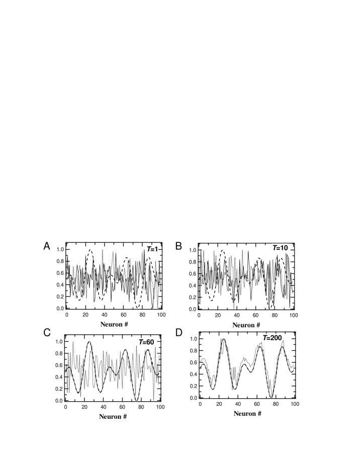
Figure 3: The local field $\textbf{u}=\mbox{\boldmath$\xi$}+\cal{W}\textbf{x}$ (thin full line) and the real part of the first eigenvector of the Jacobian matrix (thin dotted line) converge to the input pattern $\xi$ (thick dashed line) at intermediate-to-long learning epochs. Snapshot are presented at $T=1$ (A, initial conditions), $T=10$ (B), $T=60$ (C) and $T=200$ (D) learning epochs. Each curve plots averages over 50 realizations (standard deviations are omitted for clarity), vectors have been normalized to $[0,1]$ for clarity. All other parameters as in fig. 1

IV Functional viewpoint

Pattern recognition is one of the functional properties of RRNNs. In our terms, a pattern is “learned” when its presentation (or removal) induces a bifurcation . Moreover, this effect must be acquired via learning, selective (i.e. only the presented pattern is learned) and robust (i.e. a noisy version of the learned pattern should lead to an attractor similar to the one reached after presentation of the learned pattern). We now proceed to an analysis of the effect of pattern removal, as a simple indicator of the functional properties of the network. A deeper investigation of the functional properties of the network is out of the scope of the present study and will be the subject of future works.
Label by x (resp. u) the neuron firing rate (resp. local field) obtained when the (time constant) input pattern $\xi$ is applied to the network (see eq. 1) and by $\textbf{x}^{\prime}$ (resp. $\textbf{u}^{\prime}$) the corresponding quantities when $\xi$ is removed ($\mbox{\boldmath$\xi$}=0$). The removal of $\xi$ modifies the attractor structure and the average value of any observable $\phi$ (though the amplitude of this change depends on $\phi$). More precisely call:

$$\Delta^{(T)}\left[\phi\right]=\left\langle\phi(\textbf{x}^{\prime})\right\rangle^{(T)}-\left\langle\phi(\textbf{x})\right\rangle^{(T)}$$ (24)

where $\left\langle\phi(\textbf{x}^{\prime})\right\rangle^{(T)}$ is the (time) average value of $\phi$ without $\xi$ and $\left\langle\phi(\textbf{x})\right\rangle^{(T)}$ the average value in the presence of $\xi$. Two cases can arise.
In the first case, the system is away from a bifurcation point and removal results in a variation of $\Delta^{(T)}\left[\phi\right]$ that remains proportional to $\xi$ provided $\xi$ is sufficiently small (remember here that the present network admits a single attractor at a given learning epoch). Albeit common for non-chaotic dynamics, we emphasize that this statement still holds for chaotic dynamics. This has been rigorously proven for uniformly hyperbolic systems, thanks to the linear response theory developed by Ruelle Ruelle (1999). In the present context, the linear response theory predicts that the variation of the average value of u is given by Cessac and Sepulchre (2006, 2007):

$$\Delta^{(T)}\left[\textbf{u}\right]=-\chi^{(T)}\mbox{\boldmath$\xi$}$$ (25)

where

$$\chi^{(T)}=\sum_{n=0}^{\infty}\left\langle D\textbf{F}^{n}\right\rangle^{(T)}$$ (26)

is a matrix, whose entries can be written:

$$\chi_{ij}^{(T)}={\cal I}+\sum_{n=1}^{+\infty}\sum_{\gamma_{ij}(n)}\prod_{l=1}^{n}W_{k_{l}k_{l-1}}\left\langle\prod_{l=1}^{n}f^{\prime}(u_{k_{l-1}}(l-1))\right\rangle^{(T)}$$ (27)

where the sum $\sum_{\gamma_{ij}(n)}$ holds on every possible path $\gamma_{ij}(n)$ of length $n$, connecting neuron $k_{0}=j$ to neuron $k_{n}=i$, in $n$ steps.
Note therefore that $\Delta^{(T)}\left[\textbf{u}\right]=-\mbox{\boldmath$\xi$}-M^{(T)}\mbox{\boldmath$\xi$}$ where the matrix $M^{(T)}=\sum_{n=1}^{\infty}\left\langle D\textbf{F}^{n}\right\rangle^{(T)}$ integrates dynamical effects. A slight variation of $u_{i}$ at $t=0$ implies a reorganization of the dynamics which results in a complex formula for the variation of $\left\langle\textbf{u}\right\rangle^{(T)}$, even if the dominant term is $\xi$, as expected. More precisely, as emphasized several times above, one remarks that each path in the sum $\sum_{\gamma_{ij}(n)}$ is weighted by the product of a topological contribution depending only on the weights $W_{ij}$ and on a dynamical contribution. The weight of a path $\gamma_{ij}$ depends on the average value of $\left\langle\prod_{l=1}^{n}f^{\prime}(u_{k_{l-1}}(l-1))\right\rangle^{(T)}$ thus on correlations between the state of saturation of the units $k_{0},\dots,k_{n-1}$ at times $0,\dots,n-1$.
Eq. 25 shows how the effects of pattern removal are complex when dealing with a chaotic dynamics. However, the situation is much easier mathematically in the simplest case where dynamics have converged to a stable fixed point $\textbf{u}^{\ast(T)}$ (resp. $\textbf{x}^{\ast(T)}$). In this case, eq. (25) reduces to:

$$\Delta^{(T)}\left[\textbf{u}\right]=-\sum_{n=0}^{\infty}\left({\cal W}^{(T)}\Lambda(\textbf{u}^{\ast})\right)^{n}\mbox{\boldmath$\xi$}$$ (28)

Calling $\lambda_{k},{\bf v}_{k}$ the eigenvalues and eigenvectors of ${\cal W}^{(T)}\Lambda(\textbf{u}^{\ast(T)})$, ordered such that $|\lambda_{N}|\leq|\lambda_{N-1}|\leq|\lambda_{1}|<1$ one obtains:

$$\Delta^{(T)}\left[\textbf{u}\right]=-\sum_{k=1}^{N}\frac{\left({\bf v}_{k},\mbox{\boldmath$\xi$}\right)}{1-\lambda_{k}}{\bf v}_{k}$$ (29)

where $\left(\;,\;\right)$ denotes the usual scalar product. Actually, this result can easily be found without using linear response, by a simple Taylor expansion (see appendix E). The response is then proportional to $\xi$ but becomes arbitrary large when $\lambda_{1}$ tends to $1$ and provided that $\left({\bf v}_{1},\mbox{\boldmath$\xi$}\right)>0$. This analysis can be formally extended to the general case (i.e. including chaos, eq. 26) but is delicate enough to deserve a treatment by its own and will be the scope of a forthcoming paper. Here, we simply want to make the following argument. From the analysis above, we expect pattern removal to have a maximal effect at “the edge of chaos”, namely when the (average) value of the spectral radius of $D\textbf{F}_{\textbf{x}}$ is close to $1$. As mentioned above, the effects are however more or less prominent according to the choice of the observable $\phi$. We empirically found that the effects were particularly prominent with the following quantity:

$$\Delta^{(T)}[\Lambda]=\frac{1}{N}\sqrt{\sum_{i=1}^{N}\left(\left\langle\Lambda_{ii}(\textbf{u})\right\rangle^{(T)}-\left\langle\Lambda_{ii}(\textbf{u}^{\prime})\right\rangle^{(T)}\right)^{2}}$$ (30)

Indeed, $\Lambda_{ii}=f^{\prime}(u_{i})$ is maximal when the local field of $i$ falls in the central pseudo-linear part of the transfer function, hence where neuron $i$ is the most sensitive to its input. Hence $\Delta^{(T)}[\Lambda]$ measures how neuron excitability is modified when the pattern is removed. The evolution of $\Delta^{(T)}[\Lambda]$ during learning following rule eq.(5) is shown on fig. 4 (full lines) for two values of the passive forgetting rate $\lambda$. $\Delta^{(T)}[\Lambda]$ is found to increase to a maximum at early learning epochs, while it vanishes afterwards. Interestingly, comparison with the decay of the leading eigenvalue of the Jacobian matrix, $\mu_{1}$ (dotted lines) shows that the maximal values of $\Delta^{(T)}[\Lambda]$ are obtained when $|\mu_{1}|=|\lambda_{1}|$ is close to $1$. Hence, these numerical simulations confirm that sensitivity to pattern removal is maximal when the leading eigenvalue is close to $1$. Therefore, “Hebb-like” learning drives the global dynamics through a bifurcation, in the neighborhood of which sensitivity to the input pattern is maximal. This property may be crucial regarding memory properties of RRNNs, which must be able to detect, through their collective response, whether a learned pattern is present or absent. This property is obtained at the frontier where the strange attractor begins to destabilize ($|\mu_{1}|=1$), hence at the so-called “edge of chaos”.

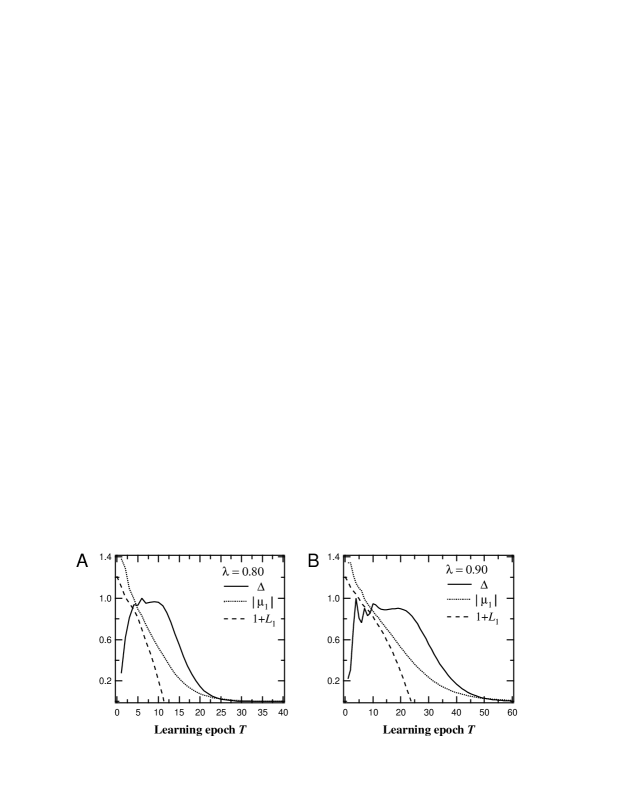
Figure 4: The network sensitivity to the input pattern is maximal close to a bifurcation. The evolution of the average value for the spectral radius of $D\textbf{F}_{\textbf{x}}^{(T)}$ during learning (dotted line) is plotted together with the sensitivity measure $\Delta^{(T)}[\Lambda]$ (full line) for $\lambda=0.80$ (A) or $0.90$ (B). The panels also display the corresponding evolution of the largest Lyapunov exponent $L_{1}$, plotted as $1.0+L_{1}$ for obvious comparison purpose (dashed line). The values of $\Delta^{(T)}[\Lambda]$ are normalized to the $[0-1]$ range for comparison purposes. Each value is an average over 50 realizations (standard deviations are omitted for clarity). All other parameters were as in fig. 1

We showed in section III.1 that the Hebbian learning rules studied here contract the spectral radius of $D\textbf{F}_{\textbf{x}},\forall\textbf{x},$ so that the latter crosses the value $1$ at some learning epoch. Thus, $1$ is ensured to be an eigenvalue of $D\textbf{F}_{\textbf{x}}$ at some point . The evolution of $v_{1}$, the eigenvector associated to the leading eigenvalue of the Jacobian matrix $\mu_{1}$, is less obvious. We plot on fig. 3 (dotted lines) the evolution of its real part during numerical simulations (actually, its imaginary part vanishes after just a couple of learning epochs). It is clear from numerical simulations that the possibility of a vanishing projection of the input pattern $\xi$ (thick dashed line) on $v_{1}$ can be ruled out (the two vectors are not orthogonal). The tendency is even opposite, i.e. $v_{1}$ is found to align on the input pattern at long learning epochs ($T\gtrsim 100$; note that we were not able to find a satisfactory explanation for this alignment).

V Discussion

The coupled dynamical system studied in the present paper (eqs.(1) and (2)) is based on several simplifying assumptions that allowed the rigorous mathematical study we have presented. However, many of the results we obtain remain valid when some of these assumptions are relaxed to improve biological realism. Here, we give a brief overview of the related arguments. As already stated in the introduction, we do not pretend to encompass the spectrum of complexity and richness of biological learning and plasticity rules Kim and Linden (2007). However, the present study focuses on the major type of synaptic plasticity (i.e Hebbian plasticity), which is generally considered as the principal cellular basis of behavioral learning and memory.
The learning rule we study here eq.(2) includes a term that allows passive forgetting ($\lambda<1$). This possibility is supported by a body of experimental data that shows that synaptic weights decay exponentially toward their baseline after LTP, in the absence of subsequent homo- or hetero-synaptic LTD, with time constants from seconds to days  Abraham et al. (1994); Brager et al. (2003); Abraham et al. (2002). A plausible molecular mechanism for this passive behavior has been recently proposed, which relies on the operation of kinase and phosphatase cycles that are systematically implicated in learning and memory Delord et al. (2007). Our theoretical results predict that learning-induced reduction of dynamics complexity can still arise in the limit case of $\lambda=1$. Indeed, numerical simulations of Hebbian learning rules devoid of passive forgetting (i.e. with $\lambda=1$) have clearly evidenced a reduction of the attractor complexity during learning Berry and Quoy (2006); Siri et al. (2006). In this case, the reduction of the attractor complexity is provoked by an increase of the average saturation level of the neurons, in agreement with our present analytical results. As a matter of fact, the question is not so much to know what exactly is the value of $\lambda$ in real neural networks, but how the characteristic time scale $\frac{1}{|\log(\lambda)|}$ compares to other time scales in the system.
Another assumption of the generic Hebbian rule we study is that $\Gamma_{ij}=0$ whenever the presynaptic neuron is silent. As already mentioned section II.1, an interpretation of this assumption is that this learning rule excludes heterosynaptic LTD. To assess the impact of this form of synaptic depression in the model, we ran numerical simulations using a variant of eq.(5) in which the Heavyside term (that forbids heterosynaptic LTD) was omitted. The results of these simulations (not shown) were in agreement with all the analytical results supported here, including those on spectral radius contraction. In agreement with these numerical simulations, our analytical results on the contraction of the spectral radius are expected to remain valid when heterosynaptic LTD is accounted for, but this would require extending the model definition and further mathematical developments that are out of the scope of the present study.
The effects of Hebbian learning were studied here in a completely connected, one population (i.e. each neuron can project both excitatory and inhibitory synapses) chaotic network. While this hypothesis allows a rigorous mathematical treatment, it is clearly a strong idealization of biological neural networks. However, we have tested the analytical predictions obtained here with numerical simulations of a chaotic recurrent neural network with connectivity mimicking cortical micro-circuitry, i.e. sparse connectivity and distinct excitatory and inhibitory neuron populations. These simulations unambiguously demonstrated that our analytical results are still valid in these more realistic conditions Siri et al. (2007).
From a functional point of view, we have shown that the sensitivity to the learned pattern is maximal at the edge of chaos. Starting from chaotic dynamics, this regime is reached at intermediate learning epochs. However, longer learning times result in poorer dynamical regimes (e.g. fixed points) and the loss of sensitivity to the learned pattern. Additional plasticity mechanisms like synaptic scaling  Turrigiano et al. (1998) or intrinsic plasticity ref  Daoudal and Debanne (2003) may constitute interesting biological processes to maintain the network in the vicinity of the edge of chaos and preserve a state of high sensitivity to the learned pattern. Such possibilities are currently under investigation in our group.

Appendix A Definitions.

Dealing with chaotic systems, one is faced with the necessity to defining indicators measuring dynamical complexity. There are basically two families of indicators: one is based on topological properties (e.g. topological entropy), the other is based on statistical properties (e.g. Lyapunov exponents or Kolmogorov-Sinai entropy). The latter family can easily be accessed numerically or experimentally by time averages of relevant observables along typical trajectories of the dynamical system. However, to this aim, one has to assume a strong ergodic property: the time average of observables, along trajectories corresponding to initial conditions drawn at random with respect to a probability distribution having a density (with respect to the Lebesgue measure), is constant (it does not depend on the initial condition). This property is far from being evident. Actually, we are not able to prove it in the present context. On mathematical grounds, it corresponds to the following assumption.

Assumption 1

Call $\mu_{L}$ is the Lebesgue measure on $[0,1]^{N}$ and let $\textbf{F}^{\ast t}\mu_{L}$ the image of $\mu_{L}$ under $\textbf{F}^{t}$. We assume that the following limit exists:

$$\rho^{(T)}=\lim_{\tau\to\infty}\frac{1}{\tau}\sum_{t=1}^{\tau}\textbf{F}^{\ast t}\mu_{L}$$ (31)

where the probability measure $\rho^{(T)}$ is called “the Sinai-Ruelle-Bowen (SRB) measure at learning epoch $T$” Sinai (1972); Ruelle (1978); Bowen (1975). Under this assumption the following holds. Let $\phi:[0,1]^{N}\to{\sf I\!R}^{N}$ be some suitable (measurable) function. Then the time average:

$$\bar{\phi}[{\textbf{x}^{(T)}}(0)]\stackrel{{\scriptstyle\rm def}}{{=}}\lim_{\tau\to\infty}\frac{1}{\tau}\sum_{t=1}^{\tau}\phi({{\textbf{x}^{(T)}}(t)}),$$ (32)

where $\textbf{x}(t)=\textbf{F}^{t}(\textbf{x})$, is equal to the ensemble average:

$$\left<\phi\right>^{(T)}\stackrel{{\scriptstyle\rm def}}{{=}}\int_{[0,1]^{N}}\phi(\textbf{x})\rho^{(T)}(d\textbf{x}),$$ (33)

for Lebesgue-almost every initial condition ${\textbf{x}^{(T)}}(0)$.

In other words, time average and ensemble average are identical on practical grounds. The use of $\rho^{(T)}$ is required to prove the mathematical results below while time average is what we use for numerical simulations.

Note that in doing so, we have constructed a family of probability distributions $\rho^{(T)}$ that depends on the learning epoch $T$. $\rho^{(T)}$ provides statistical information about the attractor structure. A prominent example is the maximal Lyapunov exponent. Let $\textbf{x}\in[0,1]^{N}$, ${\bf v}\in{\sf I\!R}^{N}$ and $\rho$ be an SRB measure. Then, the largest Lyapunov exponent is given by:

$$L_{1}^{(T)}=\lim_{t\to\infty}\lim_{\|{\bf v}\|\to 0}\frac{1}{t}\log\left(\frac{\|D\textbf{F}^{t}_{\textbf{x}}{\bf v}\|}{\|{\bf v}\|}\right)$$ (34)

Its value is constant for $\rho^{(T)}$ almost every x. (Note indeed that the LHS does not depend on x, while the RHS does. This is a direct consequence of the assumption that $\rho^{(T)}$ is an SRB measure).

Appendix B Asymptotic behaviors

In the specific learning rule eq.(5) used in our numerical simulations, $\Gamma_{ij}=m_{i}m_{j}H(m_{j})$. Thus

$$\|\Gamma\| = \mathrm{sup}_{x}\frac{\|\Gamma\textbf{x}\|}{\|\textbf{x}\|}$$ (35)

$$= \mathrm{sup}_{x}\frac{\|\mathbf{m}\left[\mathbf{m}H(\mathbf{m})\right]^{+}\textbf{x}\|}{\|\textbf{x}\|}$$ (36)

$$\leq \|\mathbf{m}\|\|\left[\mathbf{m}H(\mathbf{m})\right]^{+}\|$$ (37)

$$\leq \left(\sum_{i=1}^{N}m_{i}^{2}\right)^{1/2}\left(\sum_{j=1,m_{j}>0}^{N}m_{j}^{2}\right)^{1/2}$$ (38)

$$\leq \sqrt{N}\sqrt{N}\phi^{1/2}$$ (39)

$$\leq N\sqrt{\phi}$$ (40)

where $\left[{\bf v}\right]^{+}$ denotes the transpose of vector ${\bf v}$, $\sum_{j=1,m_{j}>0}$ denotes a sum restricted to the active neurons and $\phi$ is the fraction of active neurons. Hence

$$\|\Gamma^{(T)}\|\leq N\sqrt{\phi^{(T)}}$$ (41)

If (as observed in our numerical simulations) $\phi^{(T)}$ tends to a stationary value $\phi^{(\infty)}$ then

$$\|\Gamma^{(T)}\|\leq N\sqrt{\phi^{(\infty)}}$$ (42)

Hence $\Gamma$ is bounded in the specific case of eq.(5) by a constant $N\sqrt{\phi^{(\infty)}}$.

More generally, $\|\Gamma\|$ is bounded provided that the function $h$ in (3) is bounded as well.

Appendix C Proof of theorem 1

Let ${\bf v},\textbf{x}\in{\sf I\!R}^{N}$. Denote by $\textbf{x}(t)=\textbf{F}^{t}(\textbf{x})$, and ${\bf v}(t)=D\textbf{F}_{\textbf{x}(t)}.D\textbf{F}^{t-1}_{\textbf{x}}.{\bf v}$, ${\bf v}(0)={\bf v}$. From the chain rule:

$$\frac{\|D\textbf{F}_{\textbf{x}}^{t}{\bf v}\|}{\|{\bf v}\|}=\frac{\|D\textbf{F}_{\textbf{x}(t)}{\bf v}(t-1)\|}{\|{\bf v}(t-1)\|}\frac{\|{\bf v}(t-1)\|}{\|{\bf v}\|}$$

$$=\frac{\|D\textbf{F}_{\textbf{x}(t)}{\bf v}(t-1)\|}{\|{\bf v}(t-1)\|}\frac{\|D\textbf{F}_{\textbf{x}(t-1)}{\bf v}(t-2)\|}{\|{\bf v}(t-2)\|}\dots\frac{\|D\textbf{F}_{\textbf{x}(1)}{\bf v}\|}{\|{\bf v}\|}$$

Therefore:

$$L_{1}^{(T)}=\lim_{t\to\infty}\lim_{\|{\bf v}\|\to 0}\frac{1}{t}\sum_{n=1}^{t}\log\left(\frac{\|D\textbf{F}_{\textbf{x}(n)}{\bf v}(n-1)\|}{\|{\bf v}(n-1)\|}\right).$$

Since $\|A{\bf v}\|\leq\|A\|\|{\bf v}\|$ :

$$L_{1}^{(T)}\leq\lim_{t\to\infty}\frac{1}{t}\sum_{n=1}^{t}\log\left(\|D\textbf{F}_{\textbf{x}(n)}\|\right)=\left<\log\left(\|D\textbf{F}_{\textbf{x}}\|\right)\right>^{(T)}\ \rho^{(T)}-\mbox{almost surely}.$$

But since $D\textbf{F}_{\textbf{x}}=\Lambda(\textbf{u}){{\cal W}}$, we have $\|D\textbf{F}_{\textbf{x}}\|\leq\|{{\cal W}}\|\|\Lambda(\textbf{u})\|\leq\|{{\cal W}}\|\max_{i}(f^{\prime}(u_{i})$.

Appendix D Local fields

Fix x and the time epoch $T$. Set $\textbf{u}={\cal W}^{(T)}\textbf{x}+\mbox{\boldmath$\xi$}$. The average of u, $\left\langle\textbf{u}\right\rangle^{(T)}$ is defined either by the time average (32) or by the ensemble average (33). However, since ${\cal W}^{(T)}$ is constant during a given learning epoch one has:

$$\left\langle\textbf{u}\right\rangle^{(T)}={\cal W}^{(T)}\left\langle\textbf{x}\right\rangle^{(T)}+\mbox{\boldmath$\xi$},\quad\forall T.$$ (43)

Therefore:

$$\left\langle\textbf{u}\right\rangle^{(T+1)}={\cal W}^{(T+1)}\left\langle\textbf{x}\right\rangle^{(T+1)}+\mbox{\boldmath$\xi$}=(\lambda{\cal W}^{(T)}+\frac{\alpha}{N}\Gamma^{(T)})(\left\langle\textbf{x}\right\rangle^{(T)}+\delta\rho^{(T+1)}(\textbf{x}))+\mbox{\boldmath$\xi$},$$

where $\delta\rho^{(T+1)}(\textbf{x})\stackrel{{\scriptstyle\rm def}}{{=}}\left\langle\textbf{x}\right\rangle^{(T+1)}-\left\langle\textbf{x}\right\rangle^{(T)}$ is the difference of the average value of x between learning epochs $T+1$ and $T$.

Thus:

$$\left\langle\textbf{u}\right\rangle^{(T+1)}=\lambda\left\langle\textbf{u}\right\rangle^{(T)}+(1-\lambda)\mbox{\boldmath$\xi$}+\lambda{\cal W}^{(T)}\delta\rho^{(T+1)}(\textbf{x})+\frac{\alpha}{N}\Gamma^{(T)}\left\langle\textbf{x}\right\rangle^{(T+1)},$$

and by recurrence:

$$\left\langle\textbf{u}\right\rangle^{(T+1)}=\lambda^{T}\left\langle\textbf{u}\right\rangle^{(1)}+(1-\lambda^{T})\mbox{\boldmath$\xi$}+\lambda\sum_{n=1}^{T}\lambda^{T-n}{\cal W}^{(n)}\delta\rho^{(n+1)}(\textbf{x})+\frac{\alpha}{N}\sum_{n=1}^{T}\lambda^{T-n}\Gamma^{(n)}\left\langle\textbf{x}\right\rangle^{(n+1)}$$ (44)

Appendix E Proof of eq.(29)

Call $\textbf{u}^{\ast(T)}$ ($\textbf{u}^{{}^{\prime}\ast(T)}$) the fixed point (for the variable u) with (without) $\xi$. We have:

$$\textbf{u}^{{}^{\prime}\ast(T)}={\cal W}\textbf{F}(\textbf{u}^{{}^{\prime}\ast(T)})$$

and:

$$\textbf{u}^{\ast(T)}={\cal W}\textbf{F}(\textbf{u}^{\ast(T)})+\mbox{\boldmath$\xi$}$$

Therefore:

$$\textbf{u}^{{}^{\prime}\ast(T)}-\textbf{u}^{\ast(T)}=\delta\textbf{u}^{(T)}={\cal W}\left[\textbf{F}(\textbf{u}^{\ast(T)}+\delta\textbf{u}^{(T)})-\textbf{F}(\textbf{u}^{\ast(T)})\right]-\mbox{\boldmath$\xi$}.$$

A series expansion yields, to the linear order:

$$({\cal I}-{\cal W}\Lambda(\textbf{u}^{(T)}))\delta\textbf{u}^{(T)}=-\mbox{\boldmath$\xi$}$$

Decomposing on the eigenbasis ${\bf v}_{k}$ of ${\cal W}\Lambda(\textbf{u}^{(T)})$ we obtain:

$$(1-\lambda_{k})(\delta\textbf{u}^{(T)},{\bf v}_{k})=-(\mbox{\boldmath$\xi$},{\bf v}_{k})$$ (45)

which corresponds to eq. (29) provided $|\lambda_{k}|<1$ (ensuring that the matrix ${\cal I}-{\cal W}\Lambda(\textbf{u}^{(T)})$ is invertible).

Appendix F Jacobian matrix and feedback loops background

Assume that we slightly perturb at time $t$ the state of neuron $j$ with a small perturbation (e.g. $x_{j}(t)\to x_{j}(t)+\delta_{j}(t)$). Then the effect of this change on neuron $i$, at time $t+1$ is given by $x_{i}(t+1)=f\left(\sum_{k=1}^{N}W_{ik}x_{k}(t)+\xi_{i}+W_{ij}\delta_{j}(t)\right)$. One can perform a Taylor expansion of this expression in powers of $W_{ij}\delta_{j}(t)$. To the linear order the effect is given by $f^{\prime}(u_{i}(t))W_{ij}\delta_{j}(t)$. To each Jacobian matrix $D\textbf{F}_{\textbf{x}}$ one can associate a graph, called “the graph of linear influences”. such that there is an oriented edge $j\rightarrow i\quad\mathrm{iff}\quad\frac{\partial f(u_{i})}{\partial x_{j}}\neq 0$. The edge is positive if $\frac{\partial f(u_{i})}{\partial x_{j}}>0$ and negative if $\frac{\partial f(u_{i})}{\partial x_{j}}<0$. An important remark is that this graph depends on the current state x, contrarily to the weights matrix which is a constant inside a given learning epoch. This has important consequences. Indeed, in our case since $\frac{\partial F_{i}}{\partial x_{j}}=f^{\prime}(u_{i})W_{ij}$, the edge $j\to i$ in the graph of linear influences can be very small even if the synaptic weight $W_{ij}$ is large. It suffices that $|u_{i}|$ be large. This effect, due to the saturation of the transfer function $f$, is prominent in the subsequent studies.
We have now the following situation: “above” (in the tangent bundle) each point x, there is graph. This graph contains circuits or feedback loops. If $e$ is an edge, denote by $o(e)$ the origin of the edge and $t(e)$ its end. Then a circuit is a sequence of edges $e_{1},...,e_{k}$ such that $o(e_{i+1})=t(e_{i})$, $\forall i=1...k-1$, and $t(e_{k})=o(e_{1})$. Such a circuit is positive (negative) if the product of its edges is positive (negative). A positive circuit basically yields (to the linear order) a positive feedback that induces an increase of the activity of the neurons in this circuit. Obviously, there is no exponential increase since rapidly nonlinear terms will saturate this effect. It is thus expected that positive loops enhance stability.

A particularly prominent example of this is well known in the framework of continuous time neural networks models and also in genetic networks. It is provided by so-called “cooperative systems”. A dynamical system is called cooperative if $\frac{\partial f(u_{i})}{\partial x_{j}}({\textbf{x}})\geq 0,\forall i\neq j$. Therefore, in this case, all edges are positive edges, whatever the state of the neural network and all circuits are positive. Cooperative systems preserve the following partial order ${\bf x}\leq{\bf y}\Leftrightarrow x_{i}\leq y_{i},\ i=1\dots N$. Thus ${\bf{x}(0)}\leq{\bf{y}(0)}\Rightarrow{\bf{x}(t)}\leq{\bf{y}(t)},\ \forall t>0$ (this corresponds to the positive feedback discussed above). From these inequalities, Hirsch Hirsch (1989) proved that for a two dimensional cooperative dynamical system, any bounded trajectory converges to a fixed point. In larger dimension, one needs moreover a technical condition on the Jacobian matrix: it must be irreducible. Then Hirsch proved that the $\omega$-limit set of almost every bounded trajectory is made of fixed points. Note that this result holds when $f$ is nonlinear.

On the opposite, negative loops usually generate oscillations. For example, the second Thomas conjecture Thomas (1981), proved by Gouzé Gouzé (1998) under the hypothesis that the sign of the Jacobian matrix elements do not depend on the state, states that “A negative loop is a necessary condition for a stable periodic behavior”. In our model, negative loop generate oscillations provided that the nonlinearity $g$ is sufficiently large. This can be easily figured out by considering a system with 2 neurons. A necessary condition to have a Hopf bifurcation giving rise to oscillations is $W_{12}W_{21}<0$, but the bifurcation occurs only when $g$ is large enough.

References

- Abraham et al. (1994) Abraham, B., W.C. Christe, B. Logan, P. Lawlor, , and M. Dragunow, 1994, Proc. Natl. Acad. Sci. USA 91, 10049.
- Abraham et al. (2002) Abraham, W., B. Logan, J. Greenwood, and M. Dragunow, 2002, J. Neurosci. 22, 9626.
- Abraham and Bear (1996) Abraham, W. C., and M. F. Bear, 1996, Trends Neurosci. 19, 126.
- Atay. et al. (2006) Atay., F., T. Biyikoglu, and J. Jost, 2006, Physica. D .
- Atay et al. (2006) Atay, F., T. Biyikouglu, and J. Jost, 2006, Physica D 224, 35.
- Barahona and Pecora (2002) Barahona, M., and L. Pecora, 2002, Phys. Rev. Lett. 89, 054101.
- Bear and Abraham (1996) Bear, M., and W. Abraham, 1996, Annu. Rev. Neurosci. 19, 437.
- Berry and Quoy (2006) Berry, H., and M. Quoy, 2006, Adaptive Behavior 14, 129.
- Boccaletti et al. (2006) Boccaletti, S., V. Latora, Y. Moreno, M. Chavez, and D. U. Hwang, 2006, Physics Reports 424, 175.
- Bowen (1975) Bowen, R., 1975, Equilibrium states and the ergodic theory of Anosov diffeomorphisms (Berlin: Springer-Verlag), volume 470.
- Brager et al. (2003) Brager, D., X. Cai, and S. Thompson, 2003, Nature Neurosci. 6, 551.
- Cessac (1994) Cessac, B., 1994, J. of Physics A 27, 927.
- Cessac (1995) Cessac, B., 1995, J. de Physique 5, 409.
- Cessac and Samuelides (2007) Cessac, B., and M. Samuelides, 2007, EPJ Special topics: Topics in Dynamical Neural Networks 142(1), 7.
- Cessac and Sepulchre (2004) Cessac, B., and J. Sepulchre, 2004, Phys. Rev. E 70, 056111.
- Cessac and Sepulchre (2006) Cessac, B., and J. Sepulchre, 2006, Chaos 16, 013104.
- Cessac and Sepulchre (2007) Cessac, B., and J. Sepulchre, 2007, Physica D 225(1), 13.
- Chung (1997) Chung, F. R. K., 1997, Spectral Graph Theory (CBMS Regional Conference Series in Mathematics).
- Daoudal and Debanne (2003) Daoudal, G., and D. Debanne, 2003, Learn. Mem. 10, 456.
- Dauce et al. (1998) Dauce, E., M. Quoy, B. Cessac, B. Doyon, and M. Samuelides, 1998, Neural Networks 11, 521.
- Daucé et al. (2002) Daucé, E., M. Quoy, and B. Doyon, 2002, Biol. Cybern. 87, 185.
- Delord et al. (2007) Delord, B., H. Berry, E. Guigon, and S. Genet, 2007, PLoS Computational Biology 3(6), e124.
- Doyon et al. (1993) Doyon, B., B. Cessac, M. Quoy, and M. Samuelides, 1993, Int. Journ. of Bif. and Chaos 3(2), 279.
- Freeman (1987) Freeman, W., 1987, Biol. Cyber. 56, 139.
- Freeman et al. (1988) Freeman, W., Y. Yao, and B. Burke, 1988, Neur. Networks 1, 277.
- Gaspard (1998) Gaspard, P., 1998, Chaos, scattering and statistical mechanics (Cambridge University Press).
- Girko (1984) Girko, V., 1984, Theor. Prob. Appl 29, 694.
- Gouzé (1998) Gouzé, J., 1998, Journ. Biol. Syst. 6(1), 11.
- Grinstein and Linsker (2005) Grinstein, G., and R. Linsker, 2005, PNAS 28(102), 9948.
- Hasegawa (2005) Hasegawa, H., 2005, Phys. Rev. E. 72, 056139.
- Hebb (1948) Hebb, D., 1948, The Organization of Behaviour (John Wiley & Sons, New-York).
- Hirsch (1989) Hirsch, M., 1989, Neur. Networks 2, 331.
- Hong et al. (2002) Hong, H., B. Kim, M. Choi, and H. Park, 2002, Phys. Rev. E 65, 067105.
- Hoppensteadt and Izhikevich (1997) Hoppensteadt, F., and E. Izhikevich, 1997, Weakly Connected Neural Networks (Springer Verlag).
- Jaeger and Haas (2004) Jaeger, H., and H. Haas, 2004, Science , 78.
- Kim and Linden (2007) Kim, S., and D. Linden, 2007, Neuron 56, 582.
- Lago-Fernández et al. (200) Lago-Fernández, L. F., R. Huerta, F. Corbacho, and J. A. Sigüenza, 200, Phys. Rev. Lett. 84, 2758.
- Langton (1990) Langton, C., 1990, Physica D. 42.
- Nishikawa et al. (2003) Nishikawa, T., A. E. Motter, Y. C. Lai, and F. C. Hoppensteadt, 2003, Phys. Rev. Lett. 91.
- Ruelle (1978) Ruelle, D., 1978, Thermodynamic formalism (Reading, Massachusetts: Addison-Wesley).
- Ruelle (1999) Ruelle, D., 1999, Journ. Stat. Phys. 95, 393.
- Sinai (1972) Sinai, Y. G., 1972, Lect. Notes.in Math. 27(4), 21.
- Siri et al. (2006) Siri, B., H. Berry, B. Cessac, B. Delord, and M. Quoy, 2006, in International Conference on Complex Systems (Boston).
- Siri et al. (2007) Siri, B., M. Quoy, B. Cessac, B. Delord, and H. Berry, 2007, Journal of Physiology (Paris) 101(1–3), 138.
- Thomas (1981) Thomas, R., 1981, On the relation between the logical structure of systems and their ability to generate multiple steady states or sustained oscillations (Springer-Verlag in Synergetics), chapter Numerical methods in the study of critical phenomena, pp. 180–193.
- Tsuda (2001) Tsuda, I., 2001, Behav. Brain Sc. 24, 793.
- Turrigiano et al. (1998) Turrigiano, G., K. Leslie, N. Desai, L. Rutherford, and S. Nelson, 1998, Nature 391, 892.
- Volchenkov and Blanchard (2007) Volchenkov, D., and P. Blanchard, 2007, arXiv:0710.3566v1.