HD-THEP-07-12 24 May 2007

Strongly warped regions, also known as throats, are a common feature of the type IIB string theory landscape. If one of the throats is heated during cosmological evolution, the energy is subsequently transferred to other throats or to massless fields in the unwarped bulk of the Calabi-Yau orientifold. This energy transfer proceeds either by Hawking radiation from the black hole horizon in the heated throat or, at later times, by the decay of throat-localized Kaluza-Klein states. In both cases, we calculate in a 10d setup the energy transfer rate (respectively decay rate) as a function of the AdS scales of the throats and of their relative distance. Compared to existing results based on 5d models, we find a significant suppression of the energy transfer rates if the size of the embedding Calabi-Yau orientifold is much larger than the AdS radii of the throats. This effect can be partially compensated by a small distance between the throats. These results are relevant, e.g., for the analysis of reheating after brane inflation. Our calculation employs the dual gauge theory picture in which each throat is described by a strongly coupled 4d gauge theory, the degrees of freedom of which are localized at a certain position in the compact space.

1 Introduction

Strongly warped regions or throats are a common feature of the landscape of type IIB string theory. More specifically, local geometries which are similar to the Klebanov-Strassler throat [1] arise naturally in flux compactifications [2] (see also [3]) and the distribution of vacua favours geometries with dynamically generated large hierarchies [4]. Under certain assumptions, this can even be turned into a prediction for the statistical distribution of multi-throat configurations [5].

Multi-throat compactifications have been considered earlier [6, 7] on the basis of the simpler Randall-Sundrum model [8], which realizes the essential features of the Klebanov-Strassler throat in a 5d geometry. Cosmological implications of the energy transfer between throats have been studied by a number of authors [9, 10, 11, 12, 14, 13, 15]. An important motivation for the analysis of cosmologies with heated throats comes from the possibility of realizing brane inflation in the strongly warped region of the compact manifold [16].

In the present paper, we focus on the energy transfer between different throats in a given type IIB compactification. If one of the throats is heated during cosmological evolution, the energy is subsequently transferred to other throats or to massless fields in the unwarped bulk of the Calabi-Yau orientifold. This energy transfer proceeds in two ways. If the temperature in a given throat is high enough, it develops a black hole horizon [17, 18] and energy is lost by Hawking radiation. When the temperature drops below a critical temperature $T_{c}$, a finite throat undergoes a phase transition during which the black hole horizon is replaced by the infrared cutoff region of the throat [19, 18, 20]. Subsequently, the throat sector contains a non-relativistic gas of Kaluza-Klein (KK) modes which decay to other throats in the Calabi-Yau orientifold.

In both cases, we calculate the energy transfer rate (respectively decay rate) as a function of the AdS scales of the throats and of their relative distance. For the decay rate, we also demonstrate how to determine its dependence on angular quantum numbers of the decaying KK modes. Moreover, we extend the analysis of [6] to a genuine 10d setup (for earlier related work see [14, 13]). To this end, we consider two AdS${}_{5}\times$S⁵ throats embedded in a 6-dimensional torus. This is a simplified model, but we argue that our results remain parametrically correct also for more general geometries. As compared to [6], we find a significant suppression of the energy transfer rates if the size of the embedding Calabi-Yau orientifold is much larger than the AdS radii of the throats. This effect can be partially compensated by a small distance between the throats. These results are relevant, e.g., for the analysis of reheating after brane inflation.

It has been shown in [21, 22] that the absorption cross sections for scalars and transversely polarized gravitons by an AdS${}_{5}\times$S⁵ throat agree with those by a stack of $N$ D3-branes (for appropriate $N$). The fact that this agreement is exact in spite of the use of leading-order perturbation theory in the strongly coupled regime on the gauge theory side is explained by a non-renormalization theorem [29]. Motivated by these results, we employ the dual gauge theory picture in which each throat is described by the world-volume gauge theory on the corresponding stack of D3-branes. The world-volume theories on different D3-brane stacks are coupled by the supergravity fields in the embedding manifold. The decay and energy transfer rates then follow from the appropriate quantum-field-theory tree-level diagrams. This calculation is considerably simpler than the corresponding analysis in the gravity picture, where one has to solve multi-dimensional tunneling problems.

We will use the above equivalence of the gravity and gauge theory picture also for non-zero temperature, where the non-renormalization theorem is violated. However, as we will show, this only leads to ${\cal O}(1)$ uncertainties. The same is true for the generalization to the Klebanov-Strassler (approximate AdS${}_{5}\times$T^1,1) throat. Given that we are anyway ignorant about the detailed geometry of the bulk space and of the specific throats which may appear in realistic models, we can tolerate this uncertainty.

We emphasize that, although we refer to throats and the corresponding large-$N$ D-brane stacks throughout the text, our results also apply to stacks of fewer branes. This may be useful for the analysis of the cosmology of a standard model which resides on D-branes in the Calabi-Yau orientifold and heats up the surrounding throats.

Our paper is organized as follows. In Sect. 2, we derive the energy loss of a heated throat to another throat which is separated from the first one by a certain distance $A$ (cf. Fig. 1). This calculation is performed by modelling both throats by stacks of D3-branes and replacing the compact space by a torus. It is then straightforward to derive the energy transfer rate by summing over the contributions of bulk KK modes coupling to both throats. The resulting parametric behaviour $\sim 1/A^{8}$ of the leading term remains valid for more general 6d compact spaces and for more complicated throat geometries.

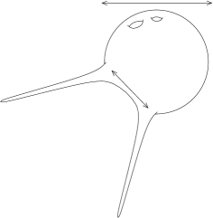
Figure 1: Two throats with radii $R_{1}$ and $R_{2}$ separated by a distance $A$ inside a Calabi-Yau orientifold of total size $L$.

Sect. 3 describes an analogous calculation for the decay rate of KK modes localized in one throat to fields in a distant throat. In the gauge theory picture, the decaying KK modes are represented by glueballs. Thus, we first derive the effective vertex for the coupling of these glueballs to bulk fields. After that, the calculation proceeds analogously to that in the previous section. Finally, we compare certain limiting cases of our result with calculations in the gravity picture and with formulae from the literature.

Our conclusions are given in Sect. 4, where we also outline possible applications of our results. A relevant integral is evaluated in the Appendix.

2 Energy transfer between two throats

Let us consider a compactification manifold containing two throats, one of which is heated to a certain temperature $T$. An interesting quantity for cosmology is the rate of energy transfer to the other throat. In the following, we will determine this rate using the description of the throats in terms of D-brane stacks. In this picture, a heated throat corresponds to a heated world-volume gauge theory. The world-volume theories on the two brane stacks are coupled by the supergravity fields in the embedding space. Thus, energy transfer between the two throats is, in this picture, due to processes of the type shown in Fig. 2, where fields in the thermal plasma on one brane stack scatter into fields on the other brane stack.

Figure 2: Feynman diagram for the scattering of fields on one brane stack into fields on another brane stack.

We will perform the corresponding calculation for a simple example – two semi-infinite AdS${}_{5}\times$S⁵ throats embedded in a 6-dimensional torus of uniform size $L$. These throats are the near-horizon geometries of black 3-branes, which in turn correspond to stacks of D3-branes (see e.g. [3, 23]). For each throat, the S⁵ radius $R$ is related to the D-brane number $N$ by

$$R^{4}=\frac{\kappa_{10}N}{2\pi^{5/2}}\,.$$ (1)

As it stands, this is not a consistent compactification since negative-charge objects are needed to absorb the flux of the branes. However, in the course of our calculation we will argue that including these and other objects (e.g. further D-branes) as well as using a different embedding manifold and a different throat geometry only leads to $\mathcal{O}(1)$ corrections.

We will restrict our calculation to the mediation by the dilaton, the Ramond-Ramond scalar and the graviton polarized parallel to the branes. In the gravity picture these three fields satisfy the same wave equation [22]. Correspondingly, in the gauge theory picture their effect in mediating energy transfer is parametrically the same. Hence, we can further restrict our calculation to one of the three fields, which we take to be the dilaton. In particular, we will not consider the effect of fermions living in the embedding manifold. In fact, in [24] the absorption cross section of dilatinos by 3-branes was calculated and found to agree with the result for the dilaton. Therefore, we expect the fermions to give parametrically the same contribution as the fields that we consider.

The (low-energy) world-volume theory on $N$ parallel D3-branes is $\smash{\mathcal{N}=4}$ U($N$) super Yang-Mills. Its field content is given by the field strength $F_{\alpha\beta}$ in the adjoint representation, six adjoint scalars $X^{i}$ corresponding to the positions of the branes, and fermionic superpartners. The coupling between the dilaton and the field strength follows from the standard 10d supergravity action with a stack of D3-branes (see e.g. [25])

$$S=\frac{1}{2\kappa_{10}^{2}}\int d^{10}x\sqrt{g}\left[{\cal R}-\frac{1}{2}(\partial\phi)^{2}+\cdots\right]+\int d^{4}x\left[-\frac{1}{4}e^{-\phi}\mbox{tr}F_{\alpha\beta}^{2}+\cdots\right]\,,$$ (2)

where, here and below, we work in the 10d Einstein frame. We ignore couplings to fermions, since they are proportional to the fermionic equations of motion and thus give no contributions to S-matrix elements [22]. Direct couplings between the dilaton $\phi$ and the scalars $X^{i}$ are absent. Canonically normalizing the dilaton kinetic term and allowing for brane fluctuations, we get [21]

$$S\supset\frac{\kappa_{10}}{2^{3/2}}\left[\int\!d^{4}x\,\phi(x,\langle\vec{X}\rangle)\,\operatorname{tr}F_{\alpha\beta}^{2}+\sum_{l}\int\!d^{4}x\frac{\kappa_{10}^{l/2}}{l!\pi^{l/4}}\left(\partial_{i_{1}}\cdots\partial_{i_{l}}\phi\right)\operatorname{tr}\left(X^{i_{1}}\cdots X^{i_{l}}\,F_{\alpha\beta}^{2}\right)\right]\!,$$ (3)

where $\smash{\langle\vec{X}\rangle}$ is the position of the brane stack. The $X^{i}$ are also defined such that their kinetic terms are canonically normalized. As can be seen from Eq. (3), couplings involving the $X^{i}$ as well as $F_{\alpha\beta}$ are suppressed by extra factors of $\smash{\kappa_{10}^{l/2}}$ and can therefore be ignored.

2.1 Energy loss rate to flat 10d space

Before we proceed, we should check whether a calculation in terms of weakly coupled gauge fields is a good approximation in the strongly coupled regime of the gauge theory. At zero temperature, this is adequate due to the non-renormalization theorem derived in [29]. However, the gauge theory is at finite temperature, which breaks supersymmetry. With supersymmetry being broken, the non-renormalization theorem from [29] cannot be expected to hold and it is not immediately clear why to trust our calculation. Therefore, we analyse a simple example in both the gauge theory and the gravity picture and compare the results. Namely, we consider a heated stack of D3-branes in flat 10d space which is dual to a non-extremal black 3-brane and calculate the energy loss rate in both pictures.

We model the heated, strongly-coupled gauge theory on the D3-brane stack by a thermal plasma of free fields. In principle, one would have to use finite temperature field theory for the calculation of the energy loss rate. However, as we are only interested in the correct order of magnitude, we can perform a zero-temperature calculation using a thermal particle distribution in the initial state. Following from Eq. (3), the cross section for scattering of two gauge bosons into one dilaton is

$$\sigma\sim\kappa_{10}^{2}\,s^{3}$$ (4)

up to $\mathcal{O}(1)$ prefactors, where $\smash{\sqrt{s}}$ is the energy of the gauge bosons in the center of mass frame. From Eq. (4), we can calculate the rate of energy loss per world-volume of the branes induced by this scattering process. This is done by thermally averaging the product of cross section and lost energy, in analogy to the standard calculations of reaction rates in a hot plasma [26, 27]:

$$\dot{\rho}=\frac{1}{2}\int d^{3}k_{1}\,d^{3}k_{2}\;f(\omega_{1})\,f(\omega_{2})\,\sigma v\,(\omega_{1}+\omega_{2})\,.$$ (5)

Here

$$f(\omega)=\frac{1}{4\pi^{3}(e^{\omega/T}-1)}$$ (6)

is the distribution function for the gauge bosons, $v$ is the relative velocity of the colliding particles, and $T$ is the temperature of the heated gauge theory. Inserting Eq. (4) into Eq. (5), we get the energy loss rate due to scattering of one gauge boson species. To get the total energy loss rate, we have to sum over all species and polarizations. In a U($N$) gauge theory there are $N^{2}$ gauge bosons. Thus, there is an extra factor of $2N^{2}$ coming from the summation. Using Eq. (1) and neglecting prefactors of order one coming from the integration in Eq. (5), we get

$$\dot{\rho}\sim R^{8}\,T^{13},$$ (7)

where $R$ is the AdS scale of the corresponding black 3-brane.

Energy loss from the non-extremal black 3-brane is due to Hawking radiation emitted by its black hole horizon. The corresponding rate per brane world-volume $\dot{\rho}$ is given by a generalization of the Hawking formula (see e.g. [25]). If we restrict ourselves to the dilaton, we get

$$\dot{\rho}=\int\frac{d^{9}k}{(2\pi)^{9}}\,\frac{v\,\omega\,\sigma_{T}(\omega)}{e^{\omega/T}-1},$$ (8)

where $v$ is the velocity of the emitted particles and $T$ is the Hawking temperature of the horizon. The absorption cross section $\sigma_{T}(\omega)$ of a dilaton by a non-extremal black 3-brane was calculated in [30]. The result is $\sigma_{T}(\omega)=\sigma_{0}(\omega)\,f(\omega/T)$, where $\omega$ is the energy of the incident dilaton, $f$ is some function of the dimensionless ratio $\omega/T$, and $\sigma_{0}(\omega)\sim\omega^{3}R^{8}$ is the absorption cross section by an extremal black 3-brane with AdS scale $R$ which was already determined in [21]. Inserting $\sigma_{T}(\omega)$ and performing the integral, we get

$$\dot{\rho}\sim R^{8}\,T^{13}.$$ (9)

Here we have neglected prefactors of order one which come in particular from the integration over $f(\omega/T)$.

Both results for the energy loss rate, Eqs. (7) and (9), agree up to $\mathcal{O}(1)$ factors. Accordingly, a weak-coupling calculation in the gauge theory picture gives the right order of magnitude. The crucial ingredient is the fact that the absorption cross section $\sigma_{T}$ of a dilaton by a non-extremal black 3-brane differs from the zero-temperature absorption cross section $\sigma_{0}$ only by a function of $\lambda\equiv\omega/T$. By gauge/gravity duality, this means that the gauge boson-dilaton vertex is corrected by a function of $\lambda$ at non-zero temperature. Accordingly, the cross section for the process in Fig. 2 that we will calculate assuming weak coupling and zero temperature has to be corrected by a function of $\lambda$. However, inserting the corrected cross section into Eq. (5) and performing the integral will just give a different ${\cal O}(1)$ prefactor, which we ignore anyway.

2.2 Energy transfer rate to a different throat

Let us now calculate the cross section for the process in Fig. 2. To this end, we need the KK expansion of the dilaton in a 6d torus,

$$\phi(x,\langle\vec{X}\rangle)=\sum_{\vec{n}\in\mathbb{Z}^{6}}\frac{1}{L^{3}}\,e^{2\pi i\vec{n}\langle\vec{X}\rangle/L}\,\Phi_{\vec{n}}(x),$$ (10)

where $L$ is the size of the torus and the expression is already evaluated at the position $\smash{\langle\vec{X}\rangle}$ of one brane stack. The mass of the $\vec{n}$th KK mode is $\smash{m_{\vec{n}}=2\pi|\vec{n}|/L}$. Inserting Eq. (10) into Eq. (3) and using $\smash{\kappa_{10}=M_{10}^{-4}}$, one sees that the vertex for the $\vec{n}$th KK mode in Fig. 2 is

$$\sim\frac{s}{M_{10}^{4}\,L^{3}}\,e^{2\pi i\vec{n}\langle\vec{X}\rangle/L}.$$ (11)

Here the energy in the center of mass frame of the gauge bosons is denoted by $\smash{\sqrt{s}}$. Let $\smash{\langle\vec{X_{1}}\rangle}$ and $\smash{\langle\vec{X_{2}}\rangle}$ be the positions of the two brane stacks inside the $T^{6}$. If we denote the relative distance of the stacks by $\smash{\vec{A}\equiv\langle\vec{X_{2}}\rangle-\langle\vec{X_{1}}\rangle}$ and introduce the shorthand $\vec{a}\equiv 2\pi\vec{A}/L$, the matrix element corresponding to the process in Fig. 2 is given by

$$\mathcal{M}\,\sim\,\frac{s^{2}}{M_{10}^{8}\,L^{6}}\,\sum_{\vec{n}\in\mathbb{Z}^{6}}\,\frac{e^{i\vec{n}\vec{a}}}{s-m_{\vec{n}}^{2}+i\epsilon}.$$ (12)

We have ignored prefactors of order one. For phenomenological purposes, we can safely assume $\smash{\sqrt{s}<L^{-1}}$. Namely, since the energy $\smash{\sqrt{s}}$ of the colliding gauge bosons is determined by the temperature $T$ of the heated gauge theory, this corresponds to $\smash{T<L^{-1}}$. If this were not the case, the gauge theory would heat up the compact manifold and the geometrical picture would be lost. Following from $\smash{\sqrt{s}<L^{-1}}$, one has $s<m_{n}^{2}$ for $n>0$ and the contribution of the energy $\smash{\sqrt{s}}$ in the propagator can be neglected for all but the zero mode. Thus, Eq. (12) simplifies to

$$\mathcal{M}\,\sim\,\frac{s^{2}}{M_{10}^{8}\,L^{4}}\,\sideset{}{{}^{\prime}}{\sum}_{\vec{n}\in\mathbb{Z}^{6}}\,\frac{e^{i\vec{n}\vec{a}}}{\vec{n}^{2}}+\frac{s}{M_{10}^{8}\,L^{6}},$$ (13)

where the prime denotes exclusion of $\smash{\vec{n}=\vec{0}}$ in the sum. Since the 4d Planck scale is determined by $M_{4}^{2}\simeq M_{10}^{8}L^{6}$, the last term in Eq. (13) simply reflects the fact that the zero mode interacts with gravitational strength. The sum, which would be UV divergent in absence of the exponential factor, is dominated by terms with large $\smash{\vec{n}}$. It can therefore be approximated by an integral:

$$\int d^{6}n\,\frac{e^{i\vec{n}\vec{a}}}{\vec{n}^{2}}\sim\frac{1}{a^{4}}.$$ (14)

The r.h. side of Eq. (14) results from the fact that the exponential function oscillates quickly for $|\smash{\vec{n}|\gtrsim a^{-1}}$ ($\smash{a\equiv|\vec{a}|}$), effectively cutting off the integral. More precisely, we evaluate a similar but more general integral, which we will need in Sect. 3.2, in the Appendix. Equation (14) follows from this integral in a particular limit, which is displayed in Eq. (45).

Inserting Eq. (14) into Eq. (13), we find

$$\mathcal{M}\,\sim\,\frac{s^{2}}{M_{10}^{8}\,A^{4}}+\frac{s}{M_{10}^{8}\,L^{6}}\,,$$ (15)

where $\smash{A\equiv|\vec{A}|}$. For an order-of-magnitude calculation, we can neglect the interference term in $\smash{|\mathcal{M}|^{2}}$. The cross section for the process in Fig. 2 then reads

$$\sigma\,\sim\,\frac{s^{3}}{M_{10}^{16}A^{8}}+\frac{s}{M_{10}^{16}L^{12}}\qquad\text{for}\qquad\sqrt{s}<L^{-1}\,.$$ (16)

Inserting this cross section into Eq. (5), we get the energy loss rate due to scattering of one particle species into another particle species. To get the total energy loss rate, we have to sum over all initial and final state species and polarizations. Let us denote with $N_{1}$ and $N_{2}$ the number of colors of the heated gauge theory and the gauge theory that is being heated, respectively. The summation then gives extra factors of $2N_{1}^{2}$ and $2N_{2}^{2}$ and we get, again neglecting prefactors of order one coming from the integration in Eq. (5),

$$\dot{\rho}\sim\frac{N_{1}^{2}N_{2}^{2}}{M_{10}^{16}A^{8}}\,T^{13}+\frac{N_{1}^{2}N_{2}^{2}}{M_{10}^{16}L^{12}}\,T^{9}.$$ (17)

Using Eq. (1), this can be written in a slightly more compact form. Denoting by $R_{1}$ and $R_{2}$ the AdS scales of the corresponding throats, we arrive at the main result of this section:

$$\dot{\rho}\sim\frac{R_{1}^{8}R_{2}^{8}}{A^{8}}\,T^{13}+\frac{R_{1}^{8}R_{2}^{8}}{L^{12}}\,T^{9}.$$ (18)

An apparent limitation of our analysis is the assumption of a simple toroidal geometry for the embedding space. This assumption was used to determine the spectrum and the couplings of higher KK modes (which determine the first term in Eqs. (13) and (18)). By contrast, the coupling of the zero mode (which determines the second term in Eqs. (13) and (18)), depends only on the size of the embedding manifold and not on its geometry. To see the relative importance of the terms more clearly, we rewrite Eq. (18) as

$$\dot{\rho}\sim\frac{R_{1}^{8}R_{2}^{8}}{A^{8}}\,T^{13}\left(1+\left(\frac{A}{L}\right)^{8}\left(L\,T\right)^{-4}\right).$$ (19)

If the throat-to-throat distance is large, $A\sim L$, the second term dominates (recall that $LT<1$) and the precise geometry is irrelevant. By contrast, for small throat separation, $\smash{A\ll L(LT)^{1/2}}$, the contribution of the KK modes is dominant. In this case, the precise geometry of the embedding manifold may in principle be relevant. However, it is then natural to assume that the curvature scale in the region between the throats is smaller than $1/A$. Furthermore, as we have already pointed out above, the sum in Eq. (13) is dominated by contributions with $|\vec{n}|\sim L/A$, corresponding to masses $\smash{m_{\vec{n}}\sim A^{-1}}$. Such modes are only sensitive to the geometry at distance scales $A$ in the vicinity of the two throats, which we just argued to be approximately flat. Thus, the order of magnitude of our result will remain correct in most relevant cases, even if the overall geometry is very different from that of a torus.

In particular, we see that O-planes and further D-brane stacks will not change our result as long as they are not too close to the two throats. Moreover, we can apply our result to situations with one Klebanov-Strassler throat and one AdS${}_{5}\times$S⁵ throat or with two Klebanov-Strassler throats as long as the curvature scale of the space in between the two throats is not much larger than $1/A$.

In order for the calculation in terms of gauge fields to be justified, the temperature of the heated throat has to be larger than its IR/confinement scale. One can then easily see from the gravity picture that the finite length of the Klebanov-Strassler throats will not change the result qualitatively. This is obvious for the heated throat since the black hole horizon hides the IR region. For the throat to which the energy is transferred, the argument is as follows: In the gravity picture, energy transfer is due to Hawking radiation, which is emitted by the heated throat and subsequently absorbed by the other throat. But only the geometry in the UV region of the throat is important for the absorption by (or, equivalently, the tunneling into) that throat.

3 Decay of KK modes between two throats

Another interesting quantity for cosmology is the rate with which KK modes localized in one throat decay to a different throat. This question has already received significant attention in the literature (see [6, 9, 10, 11, 12, 14, 13, 15]), mainly in the context of reheating after brane-antibrane inflation. However, in all cases the calculations were done in the gravity picture, whereas we will again (mainly) exploit the gauge theory point of view. This will allow us to incorporate easily the dependence on the throat radii and the distance between the throats. We compare the results from the literature with ours in Sect. 3.3.

3.1 The glueball decay vertex

We want to calculate the decay rate of glueballs on one brane stack into two gauge fields on another brane stack. As in Sect. 2, we perform the calculation for two D3-brane stacks in a 6-dimensional torus of uniform size $L$. As before, we can argue that our result provides the right order of magnitude also for more general geometries. The Feynman diagram for the process is shown in Fig. 4. Due to the non-renormalization theorem described in the introduction, we do not have to care whether the decay products will arrange into one or more glueballs. The vertex for this part of the diagram is simply the one already derived in Eq. (11). However, the other vertex between a dilaton and a glueball can not so easily be read off from the Lagrangian. Therefore, we make use of the gravity picture to calculate the decay rate in a simpler situation. From this we will determine the vertex by demanding that this decay rate agree with the gauge theory picture.

Figure 3: Feynman diagram for the decay of a glueball in one throat into fields in another throat.

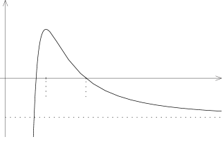
Figure 4: Potential in the effective Schrödinger equation for the dilaton in a throat.

Namely, we consider a dilaton localized in a single AdS${}_{5}\times$S⁵ throat which is embedded into flat 10d space. This is the geometry of an extremal black 3-brane, the metric being given by [31]

$$ds^{2} = f(r)^{-1/2}\,\left(-dt^{2}+dx_{1}^{2}+dx_{2}^{2}+dx_{3}^{2}\right)+f(r)^{1/2}\,\left(dr^{2}+r^{2}d\Omega_{5}^{2}\right)$$ (20)

$$\text{with}\qquad f(r)=1+\frac{R^{4}}{r^{4}}.$$

In the near-horizon region, for $\smash{r\ll R}$, the warp factor reduces to $f(r)\simeq R^{4}/r^{4}$ and the geometry is asymptotically AdS${}_{5}\times$S⁵. Far from the horizon, for $r\gg R$, the warp factor is $f(r)\simeq 1$ and the geometry is asymptotically flat 10d space. In this situation, the AdS/CFT conjecture is based on taking the near-horizon limit $r\rightarrow 0$ and $\alpha^{\prime}\rightarrow 0$, while keeping $r/\alpha^{\prime}$ fixed. This effectively reduces the geometry to the AdS${}_{5}\times$S⁵ part. In the equivalent description by a stack of D3-branes in flat space, interactions between supergravity and the world-volume theory vanish in this limit. This can be seen, e.g., from Eq. (3), since $\alpha^{\prime}\rightarrow 0$ implies $\kappa_{10}\sim g_{s}\alpha^{\prime 2}\rightarrow 0$ at finite $g_{s}$. One then identifies states in the world-volume gauge theory with eigenmodes of supergravity on AdS${}_{5}\times$S⁵.

In our considerations, however, we want to retain the asymptotically flat part of the geometry. What were previously the eigenmodes on AdS${}_{5}\times$S⁵ will then become part of the spectrum of excitations in the full geometry, including excitations outside of the throat region. This reflects the fact that, since we do not set $\alpha^{\prime}$ to zero, the gauge theory will interact with the supergravity fields in the embedding space.

Such nonvanishing interactions lead to the decay of gauge theory states, to which we refer as glueballs, into supergravity fields. This glueball decay has a simple counterpart on the gravity side. Namely, excitations in the gauge theory correspond to excitations in the throat region. The state dual to the glueball will therefore be a wave packet which is localized in the throat. Due to the different time evolution of its constituent modes, this wave packet will decohere after a certain time (see [15]). Hence, excitations will show up in the asymptotically flat region as well, which is the analogue of glueball decay.

We will now determine the decay rate of a dilaton localized in the throat into flat 10d space. To this end, we will assume the throat to be sharply cut off somewhere in the IR. Such an AdS${}_{5}\times$S⁵ throat with an IR cutoff might not exist as a solution to supergravity, but it can serve as a simple toy model capturing the relevant information. Later on we will show how to extend our results to realistic finite throats such as the Klebanov-Strassler throat [1]. On the gauge theory side, the cutoff corresponds to a deformation by a relevant operator, in which case the gauge theory has a discrete set of glueball states.

The wave equation for the dilaton is just the Laplace equation in the background geometry:

$$\partial_{M}\left(\sqrt{g}g^{MN}\partial_{N}\phi\right)=0.$$ (21)

Using Eq. (20), one gets

$$\left[r^{-5}\frac{d}{dr}\,r^{5}\,\frac{d}{dr}+m^{2}+\frac{m^{2}R^{4}}{r^{4}}-\frac{l(l+4)}{r^{2}}\right]\phi(r)=0,$$ (22)

where $l(l+4)$ is the eigenvalue of the Laplacian on S⁵ and $m^{2}$ is the eigenvalue of the 4d d’Alembertian. We will call $m$ the mass of the excitation. Choosing a new radial coordinate $\smash{z\equiv R^{2}/r}$ and introducing a redefined field $\smash{\tilde{\phi}\equiv z^{-3/2}\phi}$, we arrive at

$$\frac{d^{2}}{dz^{2}}\,\tilde{\phi}(z)+\left(m^{2}-\frac{15/4+l(l+4)}{z^{2}}+\frac{m^{2}R^{4}}{z^{4}}\right)\,\tilde{\phi}(z)=0.$$ (23)

This has the form of a Schrödinger equation, the potential being given by the term in brackets. A schematic plot of this potential is shown in Fig. 4. As one can see, a wave coming from the near-horizon region ($z\rightarrow\infty$ corresponding to $r\rightarrow 0$) has to tunnel through an effective barrier to reach the asymptotically flat region ($z\rightarrow 0$ corresponding to $r\rightarrow\infty$). The tunneling probability $\mathcal{P}$ has been calculated in [21] (see also [14]) for masses $\smash{m\ll R^{-1}}$,

$$\mathcal{P}\sim\,\left(mR\right)^{8+4l}\,,$$ (24)

where we again neglect prefactors of order one.

Although this result has been derived for a throat which is infinite in the IR direction, we can still use it for a finite throat, as long as the mass $m$ of the wave is not too small. For a throat which is cut off in the IR at $z=z_{\rm\text{\tiny IR}}$, masses are quantized in units of $m_{\rm\text{\tiny IR}}\equiv\smash{z_{\rm\text{\tiny IR}}^{-1}}$ such that $m_{n}\sim n\,m_{\rm\text{\tiny IR}}$ with $n$ an integer. The result of Eq. (24) can then be trusted as long as the wave function is not completely dominated by the unknown IR cutoff region. This will be the case if $n$ is sufficiently larger than 1.

The wave packet describing the glueball can be decomposed into a set of modes moving in the IR direction and in the UV direction. If the barrier on the UV side were impenetrable, the modes would be reflected entirely on the UV and IR side. However, since a small fraction of the incoming flux is able to penetrate the barrier, the wave leaks out of the throat. The incoming and outgoing fluxes at the barrier, $j_{\text{in}}$ and $j_{\text{out}}$, determine the tunneling probability $\mathcal{P}$ and the decay rate $\Gamma$:

$$\mathcal{P}=1-j_{\text{out}}/j_{\text{in}}\quad,\quad\Gamma=j_{\text{in}}\mathcal{P}.$$ (25)

Thus, a wave packet localized in the throat will decohere.

To determine $\Gamma$, we need solutions to Eq. (23) describing waves which are reflected back and forth between the UV barrier and the IR end of the throat. From these we can calculate the incoming flux $j_{\text{in}}$. We restrict ourselves to the case $\smash{m\ll R^{-1}}$. In particular, this means that $z_{\rm\text{\tiny IR}}\gg R$, where $z=R$ corresponds to the beginning of the throat region (cf. Eq. (20)). For $\smash{z\gg m^{-1}\gg R}$, we can neglect the last two terms in the potential, keeping only the constant term $m^{2}$. In this limit, the solution is simply given by plane waves:

$$\tilde{\phi}\simeq A\,\cos{mz}+B\,\sin{mz}.$$ (26)

The approximation is valid for $\smash{z_{\rm\text{\tiny IR}}\geq z\gg m^{-1}}\sim z_{\rm\text{\tiny IR}}/n$. If $n$ is not too small, the mode is well approximated by a plane wave in a large portion of the throat. Deviations from this form for $z\lesssim z_{\rm\text{\tiny IR}}/n$ are due to reflection at and tunneling through the effective barrier.

To calculate $j_{\text{in}}$ from Eq. (26), we have to determine the normalization of the solution in physical terms. As a simplification, we consider a complex scalar and a plane wave moving around an $S^{1}$ parametrized by $z\in[0,z_{\rm\text{\tiny IR}})$. Going to the rest frame with respect to momenta parallel to the brane and reinstating time dependence, we have

$$\tilde{\phi}=\mathcal{N}\,e^{im(z+t)}$$ (27)

for the plane wave moving towards the UV barrier. To determine the normalization constant $\mathcal{N}$, we use the standard charge density for a Klein-Gordon particle, $\smash{j^{0}=\operatorname{Im}(\tilde{\phi}^{*}\partial_{t}\,\tilde{\phi})}$. It has to be normalized according to

$$1=\int_{0}^{z_{\rm\text{\tiny IR}}}dz\,j^{0}\;\;\Rightarrow\;\;\mathcal{N}=\frac{1}{\sqrt{mz_{\rm\text{\tiny IR}}}}.$$ (28)

The flux is then given by $j_{\text{in}}=j^{z}=\operatorname{Im}(\tilde{\phi}^{*}\partial_{z}\,\tilde{\phi})$. Using the solution of Eq. (27) with the normalization of Eq. (28), we find

$$j_{\text{in}}=\frac{1}{z_{\rm\text{\tiny IR}}}=m_{\rm\text{\tiny IR}}.$$ (29)

Using this result and Eq. (24), the decay rate of a glueball follows from Eq. (25) as

$$\Gamma\sim m_{\rm\text{\tiny IR}}(mR)^{8+4l}.$$ (30)

Now that we have the decay rate in the gravity picture, we need to define a vertex $V$ in the gauge theory picture which reproduces this result. We model the coupling by a term

$${\cal L_{\rm 10d}}\,\,\supset\,\,V\,\delta^{(6)}(\vec{X}-\langle\vec{X}\rangle)\,\phi(x,\langle\vec{X}\rangle)\,{\cal G}(x)$$ (31)

in the 10d Lagrangian, where $\mathcal{G}$ denotes the glueball state with canonically normalized 4d kinetic term. Compactifying the 6 dimensions perpendicular to the brane on a torus of size $L$ for the moment and using the KK mode decomposition of Eq. (10), we get the effective 4d Lagrangian

$$\mathcal{L}_{\rm 4d}\,\supset\,\sum_{\vec{n}\in\mathbb{Z}^{6}}\left(-\frac{1}{2}\partial_{\mu}\Phi_{\vec{n}}\,\partial^{\mu}\Phi_{\vec{n}}-\frac{1}{2}m_{\vec{n}}^{2}\,\Phi_{\vec{n}}^{2}+e^{2\pi i\vec{n}\langle\vec{X}\rangle/L}\,\frac{V}{L^{3}}\,\Phi_{\vec{n}}(x)\,\mathcal{G}(x)\right)\,.$$ (32)

From this, the total decay rate of a glueball into KK modes of the dilaton follows:

$$\Gamma=\frac{1}{2\omega_{i}}\frac{1}{L^{6}}\sum_{\vec{n}\in\mathbb{Z}^{6}}\int\frac{d^{3}p_{f}}{(2\pi)^{3}}\,\frac{1}{2\omega_{f}}\,(2\pi)^{4}\,\delta^{(4)}(p_{f}-p_{i})\,|V|^{2}.$$ (33)

In this formula, $p_{f}=p_{f_{\parallel}}$ is a 4-vector characterizing the momentum of the final-state dilaton parallel to the brane, while $\omega_{i}$ and $\omega_{f}$ are the energies of the initial and final state. The 4-momentum of the decaying glueball is denoted by $p_{i}$. Introducing the dilaton momentum in the compact dimensions as $\smash{\vec{p}_{f_{\perp}}=2\pi\,\vec{n}/L}$, we can replace the sum by an integral when we go back to $L\rightarrow\infty$:

$$\frac{1}{L^{6}}\,\sum_{\vec{n}\in\mathbb{Z}^{6}}\;\longrightarrow\;\int\frac{d^{6}p_{f_{\perp}}}{(2\pi)^{6}}\,.$$ (34)

The decay rate of a glueball into a dilaton is then given by

$$\Gamma=\frac{1}{2\omega_{i}}\int\frac{d^{6}p_{f_{\perp}}}{(2\pi)^{6}}\frac{d^{3}p_{f_{\parallel}}}{(2\pi)^{3}}\,\frac{1}{2\omega_{f}}\,(2\pi)^{4}\,\delta^{(4)}(p_{f_{\parallel}}-p_{i})\,|V|^{2}\,.$$ (35)

Since the dilaton is massless, $\smash{\omega_{f}=\sqrt{|\vec{p}_{f_{\perp}}|^{2}+|\vec{p}_{f_{\parallel}}|^{2}}}$. Going to the rest frame of the glueball, $\smash{\vec{p_{i}}}=0$, and performing the momentum integrations, we arrive at

$$\Gamma=\frac{1}{2\omega_{i}}\int\frac{d^{6}p_{f_{\perp}}}{(2\pi)^{6}}\,\frac{1}{2\omega_{f}}\,(2\pi)\,\delta(\omega_{f}-\omega_{i})\,|V|^{2}\sim\omega_{i}^{3}\,|V|^{2}\,,$$ (36)

where we have used $\smash{\omega_{f}=|\vec{p}_{f_{\perp}}|}$ and neglected prefactors of order one. In its rest frame, $\omega_{i}$ is simply the mass $m$ of the glueball. Comparing with Eq. (30), we get

$$V\sim\sqrt{m_{\rm\text{\tiny IR}}m}\,\,\,m^{2+2l}R^{4+2l}.$$ (37)

3.2 Decay rate calculation in the gauge theory picture

With the effective vertex $V$ at hand, calculating the decay rate of one glueball into gauge fields living on a different brane stack is straightforward. Following from Eqs. (32) and (37), the vertex between a glueball and a KK mode of the dilaton is

$$\frac{V}{L^{3}}\,e^{2\pi i\vec{n}\langle\vec{X}\rangle/L}.$$ (38)

The other vertex in the diagram is still given by Eq. (11). Summing over all intermediate KK modes, we arrive at an expression very similar to Eq. (12):

$$\mathcal{M}\,\sim\,\frac{\sqrt{m_{\rm\text{\tiny IR}}m}\,(mR)^{4+2l}}{M_{10}^{4}\,L^{6}}\,\sum_{\vec{n}\in\mathbb{Z}^{6}}\,\frac{e^{i\vec{n}\vec{a}}}{m^{2}-m_{\vec{n}}^{2}+i\epsilon}.$$ (39)

Compared to Eq. (12), the only difference is the prefactor and the substitution of the energy $\smash{\sqrt{s}}$ of the colliding gauge bosons by the mass $m$ of the glueball.

We will analyse Eq. (39) in two different regimes, namely for $m^{-1}>L$ and for $m^{-1}\ll~{}L$. The former case is the most interesting one from a phenomenological viewpoint. As we argued in Sect. 2, we can assume that the reheating temperature $T_{\text{RH}}$ in early cosmology is smaller than $L^{-1}$. Accordingly, the mass $m$ of any relic KK modes is also restricted by $m<L^{-1}$. The latter case, on the other hand, can be easily analysed in the gravity picture as well. We will perform this cross-check in Sect. 3.3.

For $m^{-1}>L$, we can make the same simplifications as in Eq. (13) and use Eq. (14) for the sum. The decay rate of a glueball into a pair of gauge bosons follows from the standard 4d formula:

$$\Gamma\sim m^{-1}|{\cal M}|^{2}\,.$$ (40)

To get the total decay rate, we have to sum over the $N^{2}$ final state gauge bosons. If we denote by $R_{1}$ and $R_{2}$ the AdS scale of the throat containing the initial and the final state, respectively, we find

$$\Gamma\sim\frac{R_{1}^{8+4l}R_{2}^{8}}{A^{8}}\,m_{\rm\text{\tiny IR}}\,m^{8+4l}+\frac{R_{1}^{8+4l}R_{2}^{8}}{L^{12}}\,m_{\rm\text{\tiny IR}}\,m^{4+4l}.$$ (41)

Although the derivation of this decay rate assumed two AdS${}_{5}\times$S⁵ throats and a torus as embedding manifold, it can also be applied to more general geometries, according to the discussion in Sect. 2. However, for different throat geometries the dependence on the eigenvalues of the angular Laplacian is of course different. These eigenvalues entered the discussion through the tunneling probability Eq. (24), from which we determined the dilaton-glueball vertex in Eq. (37). For the example of a Klebanov-Strassler throat [1], let us outline how to determine the dilaton-glueball vertex for more general throat geometries. Away from the bottom of the throat at $r=r_{s}$, the warp factor of a Klebanov-Strassler throat is well approximated by

$$A(r)=1+\frac{R^{4}\,\ln(r/r_{s})}{r^{4}}.$$ (42)

The effective AdS scale $R$ depends on the number of fractional D3-branes at the conifold singularity. The metric is still given by Eq. (20) away from $r=r_{s}$ if one also replaces the line element $d\Omega_{5}^{2}$ of a sphere by the line element of $T^{1,1}$. For $R\gg r\gg r_{s}$, which defines the throat region, the warp factor is approximately $A\simeq R^{4}\ln(r/r_{s})/r^{4}$. For $r\gg R$, where the geometry is asymptotically a cone over $T^{1,1}$, we have $A\simeq 1$. Near $r=r_{s}$, the geometry differs considerably from Eqs. (42) and (20) and the throat is cut off by the Klebanov-Strassler region. For an order of magnitude estimate, one can neglect the logarithmic $r$ dependence of the warp factor away from $r=r_{s}$ and approximate the Klebanov-Strassler region by a sharp cut off [32]. Thus, the tunneling probability from the throat into the conical region can be (approximately) calculated from the effective Schrödinger equation, Eq. (23). The dependence on the eigenvalues of the Laplacian on $T^{1,1}$ enters through the potential, where they replace the corresponding eigenvalues $l(l+4)$ on an $S^{5}$. Moreover, for an AdS warp factor and a sharp cut off, the incoming flux is given by Eq. (29), as before. From Eq. (25), one can then determine the decay rate and match the vertex such that this decay rate is reproduced.

Let us now consider the case $m^{-1}\ll L$. We will also assume $A\ll L$ for simplicity. Recalling that $\smash{m_{\vec{n}}=2\pi|\vec{n}|/L}$ and $\vec{a}=2\pi\vec{A}/L$, we can approximate the sum in Eq. (39) by an integral,

$$\frac{1}{L^{6}}\,\sum_{\vec{n}\in\mathbb{Z}^{6}}\,\frac{e^{2\pi i\vec{A}\,\vec{n}/L}}{m^{2}-(2\pi)^{2}\vec{n}^{2}/L^{2}+i\epsilon}\;\;\;\longrightarrow\;\;\;\int\frac{d^{6}\rho}{(2\pi)^{6}}\,\frac{e^{i\vec{A}\,\vec{\rho}}}{m^{2}-\vec{\rho}^{2}+i\epsilon},$$ (43)

where $\vec{\rho}\equiv 2\pi\,\vec{n}/L$. The resulting expression is just the propagator of a massless particle in a mixed, energy-configuration-space representation, with the ‘energy’ $m$ characterizing the invariant 4-momentum. This is of course expected in the large $L$ limit, where the torus goes over to flat space and the infinite KK tower is replaced by the underlying higher-dimensional dilaton field. The integral is evaluated in the Appendix, the outcome being

$$\int\frac{d^{6}\rho}{(2\pi)^{6}}\,\frac{e^{i\vec{A}\,\vec{\rho}}}{m^{2}-\vec{\rho}^{2}+i\epsilon}\sim\frac{m^{2}}{A^{2}}\,H_{2}^{+}(mA),$$ (44)

where $H_{2}^{+}(x)=J_{2}(x)+i\,Y_{2}(x)$ is a Hankel function and we have neglected prefactors of order one. Using the asymptotic forms of the Bessel functions for large and small arguments, Eq. (44) can be simplified as follows:

$$\frac{m^{2}}{A^{2}}\,H_{2}^{+}(mA)\sim\begin{cases}\frac{m^{3/2}}{A^{5/2}}\,e^{i\,mA}&\text{for }m^{-1}\ll A\\ \frac{1}{A^{4}}&\text{for }m^{-1}\gg A\,.\end{cases}$$ (45)

Inserting these results in Eq. (39), we get the matrix elements $\mathcal{M}$ for these two cases. The corresponding partial decay rates follow from Eq. (40). Summing over all final state species, we find

$$\Gamma\sim\begin{cases}\frac{R_{1}^{8+4l}R_{2}^{8}}{A^{5}}\,m_{\rm\text{\tiny IR}}\,m^{11+4l}&\text{for }m^{-1}\ll A\\ \frac{R_{1}^{8+4l}R_{2}^{8}}{A^{8}}\,m_{\rm\text{\tiny IR}}\,m^{8+4l}&\text{for }m^{-1}\gg A\end{cases}.$$ (46)

Again, the same discussion as before applies concerning the extension to more realistic geometries. As a consistency check, we should examine, whether the appropriate limiting cases of Eqs. (41) and (46) coincide. The regions of validity of the two calculations have a common border for $A\ll m^{-1}\sim L$. Indeed, for this choice of parameters the first term in Eq. (41) dominates and the result agrees with the second line of Eq. (46).

3.3 Some calculations in the gravity picture

As in the sections before, we consider two AdS${}_{5}\times$S⁵ throats embedded in a 6-dimensional torus of uniform size $L$. The geometry is that of a multi-centered black 3-brane, the metric being

$$ds^{2}=A^{-1/2}\,\left(-dt^{2}+dx_{1}^{2}+dx_{2}^{2}+dx_{3}^{2}\right)+A^{1/2}\,\left(dx_{4}^{2}+\cdots+dx_{9}^{2}\right)$$ (47)

with

$$A(\vec{x}_{\perp})=1+\sum_{\vec{n}\in\mathbb{Z}^{6}}\left(\frac{R_{1}^{4}}{|\vec{x}_{\perp}-\vec{A}_{1}+\vec{n}L|^{4}}+\frac{R_{2}^{4}}{|\vec{x}_{\perp}-\vec{A}_{2}+\vec{n}L|^{4}}\right).$$ (48)

The positions of the two throats are denoted by $\vec{A}_{1}$ and $\vec{A}_{2}$, their AdS scales by $R_{1}$ and $R_{2}$. The vector $\smash{\vec{x}_{\perp}}$ refers to the coordinates $x_{4},\dots,x_{9}$ in the torus. The sum in the warp factor $\smash{A(\vec{x}_{\perp})}$ is due to mirror effects in the torus. Again, this is not a consistent compactfication. Including O-planes, for example, would give extra contributions to the warp factor (see [3]). We try to calculate the transition of a dilaton between different throat regions, which is the gravity counterpart to the gauge theory calculation in Sects. 3.1 and 3.2. The equation of motion for the dilaton is given in Eq. (21). Inserting Eq. (47) in Eq. (21) and using $\smash{\sqrt{g}=A^{1/2}}$, one gets

$$\partial_{n}\,\partial^{n}\,\phi+A(\vec{x}_{\perp})\,\partial_{\mu}\,\partial^{\mu}\,\phi=0.$$ (49)

The indices $\mu$ and $n$ run from 0 to 3 and from 4 to 9, respectively. Using the 4d Klein-Gordon equation, one arrives at

$$\partial_{n}\,\partial^{n}\,\phi+A(\vec{x}_{\perp})\,\,m^{2}\,\phi=0,$$ (50)

where $m$ is the kinetic energy perpendicular to the branes. Like Eq. (23), this has the form of a Schrödinger equation. Contrary to Eq. (23), however, there is no potential barrier separating the throat region and asymptotically flat space, since the potential $\smash{V=-m^{2}A(\vec{x}_{\perp})}$ is strictly negative. The difference comes from using cartesian coordinates perpendicular to the branes in Eq. (47) rather than spherical coordinates in Eq. (20). Still, a wave in the throat region, moving away from the horizon, is reflected to a large part before entering asymptotically flat space. In cartesian coordinates, however, this is due to the steepness of the potential well.

To determine the transition probability $\mathcal{P}$ of a dilaton between two throat regions, one has to solve Eq. (50) with appropriate boundary conditions. Then $\mathcal{P}$ is the ratio of incoming flux in one throat and outgoing flux in the other throat. In general, the corresponding calculation is difficult. However, if the torus is very large ($L\rightarrow\infty$) and the throats are sufficiently far apart ($A\gg\smash{m^{-1}}$), the problem effectively splits into two simpler calculations. Namely, the latter condition means that the de Broglie wavelength of the particle is small compared to the distance of the throats. A transition between two throats can then be described as a two-step process. For simplicity, we take the initial state in the first throat to be an s-wave. Only a small fraction of the outgoing flux reaches the asymptotically flat region, the probability being (cf. Eq. (24) for $l=0$)

$$\mathcal{P}_{1}\sim\left(mR_{1}\right)^{8}.$$ (51)

In between the two throats, one has a free spherical wave, approximating a plane wave near the second throat. The absorption cross section (per brane world-volume) for such a plane wave was calculated in [21]. Neglecting prefactors of order one, it reads

$$\sigma_{2}\sim m^{3}R_{2}^{8}.$$ (52)

Near the second throat, the incoming flux will be diluted by a factor of $\smash{A^{-5}}$, since the free spherical wave is expanding in 6-dimensional flat space. The absorption probability by the second throat thus is

$$\mathcal{P}_{2}\sim\frac{\sigma_{2}}{A^{5}}\sim\frac{m^{3}R_{2}^{8}}{A^{5}}.$$ (53)

The transition probability between the two throats is just the product $\mathcal{P}_{1}\mathcal{P}_{2}$. If we denote by $m_{\rm\text{\tiny IR}}$ the mass gap in the first throat, using Eqs. (25) and (29) the decay rate from the gravity calculation follows as

$$\Gamma\sim\frac{R_{1}^{8}R_{2}^{8}}{A^{5}}\,m^{11}m_{\rm\text{\tiny IR}}.$$ (54)

This is precisely what we found in Eq. (46) for $A\gg m^{-1}$ and $l=0$. The crucial ingredient is the $A^{-5}$ dependence. That it agrees in both calculations is, however, not too surprising. In the gauge theory calculation, it came from the propagator in a mixed energy-configuration-space representation (cf. Eq. (43)). The same is of course true in the above gravity calculation, although we have not stated it explicitly.

There is yet another situation where the decay rate between two throats is comparatively easy to obtain. Let us consider only one throat for the moment. We do not need to specify the precise form, but will assume that it is finite and reasonably well approximated by a slice of AdS₅ times some compact manifold $\mathcal{M}$. The prime example certainly is a Klebanov-Strassler throat, whose interpretation as a stabilized Randall-Sundrum model was given in [32]. Let us denote by $R_{1}$ the (approximate) AdS scale of the throat and by $L$ the size of the embedding manifold, whose precise geometry is again not important. One has $L\gtrsim R_{1}$, since otherwise the throat could not be glued into the manifold. If the embedding manifold is of minimal size, $L\sim R_{1}$, KK modes with masses $\smash{m_{n}\ll R_{1}^{-1}}$ cannot resolve its precise geometry. We can then describe the embedding manifold by the Planck brane in a Randall-Sundrum model. Let us consider the Kaluza-Klein expansion of the graviton in the throat. If we restrict ourselves to an s-wave with respect to the compact manifold $\mathcal{M}$ multiplying the slice of AdS₅, we can take the action from [33] obtained in the context of Randall-Sundrum phenomenology:

$$S=\int d^{4}x\;\sum_{n}\left(-\frac{1}{2}\partial_{\alpha}h_{\mu\nu}^{(n)}\,\partial^{\alpha}h^{\mu\nu(n)}-\frac{1}{2}\,m_{n}^{2}\,h_{\mu\nu}^{(n)}\,h^{\mu\nu(n)}+\frac{1}{\sqrt{2}}\frac{g_{n}}{\sqrt{M_{5}^{3}R_{1}}}\,h^{(n)}_{\mu\nu}\,T^{\mu\nu}\right).$$ (55)

The effective 5d Planck scale $M_{5}$ is determined by $M_{5}^{3}\sim M_{10}^{8}R_{1}^{5}$. We have included the coupling of the KK modes $\smash{h_{\mu\nu}^{(n)}}$ to the energy-momentum tensor $\smash{T^{\mu\nu}}$ on the Planck brane, which we will need in a moment. For KK modes with $\smash{m_{n}\ll R_{1}^{-1}}$, the masses are determined by

$$J_{1}(m_{n}/m_{\rm\text{\tiny IR}})\simeq 0\;\Rightarrow\;m_{n}\simeq\left(n+\frac{1}{4}\right)\pi\,m_{\rm\text{\tiny IR}},$$ (56)

where $\smash{m_{\rm\text{\tiny IR}}=z_{\rm\text{\tiny IR}}^{-1}}$ is the inverse conformal length of the throat (cf. Sect. 3.1) and we have used the asymptotic form for large arguments of the Bessel function $J_{1}$. This is consistent for $n$ somewhat larger than 1. The coupling constants $g_{n}$ were calculated in [33], the result being

$$g_{n}=\left(\left(\frac{Y_{1}(m_{n}R_{1})}{Y_{1}(m_{n}/m_{\rm\text{\tiny IR}})}\right)^{2}-1\right)^{-1/2}\simeq\;\sqrt{\frac{\pi}{2}}\,\sqrt{m_{n}m_{\rm\text{\tiny IR}}}\,R_{1}.$$ (57)

In the last step we have used the asymptotic forms for the Bessel function $Y_{1}$.

Let us return to the case of two throats and consider another throat in the embedding manifold. We take the throat to be AdS${}_{5}\times$S⁵ such that it can be equally well described by a stack of D3-branes. Again, its AdS scale $R_{2}$ cannot be larger than $L$, and since we have assumed $L\sim R_{1}$, one has $R_{1}\gtrsim R_{2}$. The corresponding number $N_{2}$ of D3-branes follows from Eq. (1) as $N_{2}\sim M_{10}^{4}R_{2}^{4}$. Now, when viewed from the first throat, the gauge theory on the stack of $N_{2}$ D3-branes resides on the Planck brane. Therefore, the graviton KK modes in this throat couple directly to the energy-momentum tensor of the gauge theory. Using the last term in Eq. (55), the decay of these KK modes into the other throat can be calculated as a decay into gauge fields. By the standard formula, the decay rate of a KK mode with mass $m_{n}$ into one species of gauge fields is

$$\Gamma\sim\frac{g_{n}^{2}}{M_{10}^{8}R_{1}^{6}}\,m_{n}^{3}.$$ (58)

There are $N_{2}^{2}$ gauge fields in the adjoint representation of U($N_{2}$). Summing and using Eqs. (57) and (1), the total decay rate follows:

$$\Gamma\sim\frac{R_{2}^{8}}{R_{1}^{4}}\,m_{n}^{4}\,m_{\rm\text{\tiny IR}}.$$ (59)

This result should be compared with Eq. (41) from the pure gauge theory calculation. The distance $A$ between the two throats cannot be smaller than their AdS scales $R_{1}$ and $R_{2}$. Since we have also assumed $L\sim R_{1}$ and $\smash{m_{n}\ll R_{1}^{-1}}$, the second term in Eq. (41) is dominant. Using $l=0$ for the s-wave that we have considered and $L\sim R_{1}$, we get the same result as Eq. (59), including the factor of $m_{\rm\text{\tiny IR}}$!

The above process is just the reverse of the energy loss by the heated Planck brane considered, e.g., in [27, 28]. Our calculation can also be viewed as a rephrasing, using partly the gauge theory picture and partly the gravity picture, of the tunneling calculation performed in [6]. In these papers, the decay rate of graviton KK modes between two throats was calculated in a 5d model with two AdS₅ slices which are glued together at a common Planck brane, assuming equal AdS scales $R_{1}=R_{2}$. However, besides giving the corrections due to different AdS scales, from the above derivation it is maybe more evident why the result is correct also in a genuine 10d setup.

The decay rate $\smash{\Gamma\sim(mR)^{4}\,m_{\rm\text{\tiny IR}}}$ from [6] was used in a number of papers [9, 10, 11, 12] in the context of reheating after brane-antibrane inflation. Moreover, [15] contains a careful analysis in a 5d model of effects related to the finite length of realistic throats. In this paper, the global KK modes in the two-throat system are determined. Tunneling of KK modes is then viewed as the decoherence of wave packets, which are set up in one throat. We have used this picture in Sect. 3.1.

Tunneling in a compact 10d setup with throats was considered in [13, 14]. For the case $m^{-1}>L$, a decay rate of $\smash{\Gamma\sim(mR)^{16}\,m_{\rm\text{\tiny IR}}}$ was derived, assuming that the particle has to tunnel through two barriers described by the potential in Eq. (23). We see a conceptual problem with this approach since we do not know how to justify a 1-dimensional quantum-mechanical picture (this 1 dimension being the radial coordinate) in the two-throat case. But even if we accept this description for the moment, there are further issues related to the two-barriers assumption: The barriers extend to values of $r\sim m^{-1}$ as can be seen from Fig. 4. Since $m^{-1}\gg R$ and $r$ measures the physical distance for $r\gg R$ (cf. Eq. (20)), the width of each barrier is given by $m^{-1}$. This just reflects the fact that a particle with mass $m$ has a de Broglie wavelength of $m^{-1}$. Accordingly, the particle has to tunnel through two entire barriers only if the distance $A$ between the two throats is $\sim 2m^{-1}$. Indeed, from Eq. (41) for $l=0$ and since $L>A$, we get a decay rate of $\smash{\Gamma\sim(mR)^{16}\,m_{\rm\text{\tiny IR}}}$ in this case, in agreement with [13, 14]. However, if $A$ is smaller than $\sim 2m^{-1}$, the particle has to tunnel through a smaller barrier. Correspondingly, the decay rate becomes larger, as can be seen from Eq. (41).

The case $m^{-1}\lesssim L$ (without assuming $m^{-1}\ll L$) was also considered in [13, 14]. It was found that the decay rate can be much larger than $\smash{\Gamma\sim(mR)^{16}\,m_{\rm\text{\tiny IR}}}$ if a certain resonance condition is fulfilled. We have not determined the decay rate for this case and therefore have no result to compare with. It would be interesting, though, to evaluate Eq. (39) for $m^{-1}\lesssim L$ and to see whether one can reproduce the results from [13, 14] as well as their resonance condition.

4 Conclusions and Outlook

We have determined the energy loss rate $\dot{\rho}$ of a throat which is heated to a certain temperature as well as the decay rate $\Gamma$ of single KK modes localized in a given throat. As a simplified setup we have chosen a 6-dimensional torus with two AdS${}_{5}\times$S⁵ throats. However, as we have argued in Sect. 2, our results stay parametrically correct for more general embedding manifolds and throat geometries. Especially, they are applicable for two Klebanov-Strassler throats if the curvature of the space connecting them is not larger than the inverse distance.

In earlier investigations [6, 9, 10, 11, 12, 14, 13, 15] of the decay of KK modes between throats, the decay/tunneling rate was determined from solving wave equations in a given gravity background. Most results were derived for the simple model of two AdS₅ slices, glued together at a common Planck brane. As we have explained in Sect. 3.3, this calculation is difficult to perform in a genuine 10d setup. Inspired by [21], we instead chose the dual gauge theory picture for our calculations. Namely, each AdS${}_{5}\times$S⁵ throat can be equally well described by a corresponding stack of D3-branes. Both brane stacks are coupled by the supergravity fields in the embedding space. The energy transfer rate from a heated throat then follows from simple tree-level quantum-field-theory processes. For the decay rate of throat-localized KK modes which are dual to glueballs, we first had to determine the glueball-supergravity vertex. To this end, we have calculated the decay rate of throat-localized KK modes into flat 10d space in the gravity picture. Then, we have determined the glueball-supergravity vertex by demanding that the decay rate following from this vertex give the same result. We have also presented some cross-checks from the gravity picture in Sect. 3.3.

From our analysis, we were able to determine the dependence of the energy transfer and decay rates on the distance $A$ between two throats as well as on the size $L$ of the embedding manifold. For example, this is relevant for the analysis of reheating after brane-antibrane inflation. In such models, one often considers inflation occurring in one throat, whereas the standard model branes reside at the bottom of another, longer throat. In that way, the generation of the right level of density fluctuations is reconciled with a solution of the gauge hierarchy problem à la Randall-Sundrum. For a viable reheating of the standard model sector, it is crucial that the energy from brane-antibrane annihilation is transferred efficiently into the standard model throat. This question was analysed in [9, 10, 11, 12, 14]. We find that, as long as the embedding manifold is not of minimal size, the energy transfer rate Eq. (18) is considerably lower than the rates previously derived in [9, 10, 11, 12]. Given our results, it will be interesting to reconsider reheating after brane-antibrane inflation.

Our results remain applicable if one deals with a small stack of D3-branes. An interesting setup is the following: Consider that the standard model resides on some D-branes in a given Calabi-Yau orientifold. Since they are a common feature of flux compactifications, such a manifold will typically contain several throats [5]. Modelling the standard model branes by a small stack of D3-branes, we can estimate the rate of energy loss to the throats in early cosmology from Eq. (18). According to Eq. (1), with $N$ being small, we just have to replace one factor of $\smash{R^{8}}$ by the corresponding power of the 10d Planck scale, $\smash{M_{10}^{-8}}$. The throat sectors, which are heated up in that way, may provide interesting dark matter candidates [10, 14]. Later in cosmological evolution, throat-localized KK modes may decay back to the standard model. The corresponding rate can be estimated from Eq. (41), again replacing $\smash{R_{2}^{8}}$ by $\smash{M_{10}^{-8}}$. The decay rate strongly depends on the angular momentum of the throat-localized KK modes. We have given this dependence explicitly for the angular momentum with respect to an S⁵ in an AdS${}_{5}\times$S⁵ throat. Moreover, we have outlined how to determine this dependence for other manifolds, e.g. the (approximate) T^1,1 in a Klebanov-Strassler throat. Depending on the cosmological epoch, the decaying KK modes may influence the abundances of light elements or lead to diffuse gamma-ray background radiation, both effects being strongly constrained by observations (see e.g. [36]). Along these lines it may even be possible to impose certain phenomenological constraints on multi-throat compactifications.

More generally, one may discuss several cosmological scenarios where reheating takes place either in the standard model sector or in a throat (as is the case after brane-antibrane inflation) and the standard model resides either at the bottom of a throat or somewhere in (the rest of) the Calabi-Yau orientifold. The energy transfer and decay rates that we have calculated can then be used in a set of Boltzmann equations to determine the evolution of energy densities of the standard model and throat sectors. We leave these interesting applications for future work.

Acknowledgements:         We would like to thank J. Braun, F. Brümmer, X. Chen, D. Dietrich, L. Kofman and M. Trapletti for helpful comments and discussions.

Appendix: Evaluation of the propagator

In Eq. (43), we had to evaluate the following propagator in a mixed, energy-configuration-space representation:

$$\int\frac{d^{6}\rho}{(2\pi)^{6}}\,\frac{e^{i\vec{A}\,\vec{\rho}}}{m^{2}-\vec{\rho}^{2}+i\epsilon}.$$ (60)

We perform the integral for imaginary values $m\rightarrow e^{i\pi/2}m$ and use analytic continuation. The integral changes into

$$-\int\frac{d^{6}\rho}{(2\pi)^{6}}\,\frac{e^{i\vec{A}\,\vec{\rho}}}{m^{2}+\vec{\rho}^{2}}.$$ (61)

We can then employ the identity $\smash{c^{-1}=\int_{0}^{\infty}d\tau e^{-c\tau}}$ for $\operatorname{Re}{c}>0$ and get

$$\begin{split}&\frac{-1}{(2\pi)^{6}}\int_{0}^{\infty}d\tau\int d^{6}\rho\;\;e^{i\vec{A}\,\vec{\rho}}\,e^{-(m^{2}+\vec{\rho}^{2})\tau}\\ =&\frac{-1}{(2\pi)^{6}}\int_{0}^{\infty}d\tau\,\left(\left[\int d\rho_{1}\;e^{iA_{1}\,\rho_{1}}\,e^{-\rho_{1}^{2}\tau}\right]\cdots\left[\int d\rho_{6}\;e^{iA_{6}\,\rho_{6}}\,e^{-\rho_{6}^{2}\tau}\right]e^{-m^{2}\tau}\right)\\ =&\frac{-1}{(4\pi)^{3}}\int_{0}^{\infty}d\tau\;\frac{1}{\tau^{3}}\,e^{-A^{2}/4\tau}\,e^{-m^{2}\tau}.\end{split}$$ (62)

We have used that $A^{2}=A_{1}^{2}+\cdots+A_{6}^{2}$. According to Eq. 3.471.9 in [37], this integral can be evaluated in terms of the modified Bessel function $K_{-2}\equiv K_{2}$, which yields

$$\frac{-1}{(2\pi)^{3}}\frac{m^{2}}{A^{2}}\,K_{2}(mA).$$ (63)

Following from Eq. 9.6.4 in [38], $K_{2}$ is related to the Hankel function $H_{2}^{+}=J_{2}+iY_{2}$. The above expression can be written as

$$\frac{i}{(4\pi)^{2}}\frac{m^{2}}{A^{2}}\,H^{+}_{2}(e^{i\pi/2}mA).$$ (64)

The Hankel function has a branch cut along the negative real axis. Therefore, one can analytically continue back to real values $m\rightarrow e^{-i\pi/2}m$, which gives

$$\frac{-i}{(4\pi)^{2}}\frac{m^{2}}{A^{2}}\,H^{+}_{2}(mA).$$ (65)

References

- [1] I. R. Klebanov and M. J. Strassler, “Supergravity and a confining gauge theory: Duality cascades and chiSB-resolution of naked singularities,” JHEP 0008 (2000) 052 [arXiv:hep-th/0007191].
- [2] S. B. Giddings, S. Kachru and J. Polchinski, “Hierarchies from fluxes in string compactifications,” Phys. Rev. D 66 (2002) 106006 [arXiv:hep-th/0105097].
- [3] H. L. Verlinde, “Holography and compactification,” Nucl. Phys. B 580, 264 (2000) [arXiv:hep-th/9906182].
-
[4]
F. Denef and M. R. Douglas, “Distributions of
flux vacua,” JHEP 0405, 072 (2004) [arXiv:hep-th/0404116];
A. Giryavets, S. Kachru and P. K. Tripathy, “On the taxonomy of flux vacua,” JHEP 0408 (2004) 002 [arXiv:hep-th/0404243];
J. P. Conlon and F. Quevedo, “On the explicit construction and statistics of Calabi-Yau flux vacua,” JHEP 0410 (2004) 039 [arXiv:hep-th/0409215];
T. Eguchi and Y. Tachikawa, “Distribution of flux vacua around singular points in Calabi-Yau moduli space,” JHEP 0601 (2006) 100 [arXiv:hep-th/0510061]. -
[5]
A. Hebecker and J. March-Russell, “The
ubiquitous throat,”
arXiv:hep-th/0607120. -
[6]
S. Dimopoulos, S. Kachru, N. Kaloper,
A. E. Lawrence and E. Silverstein, “Generating small numbers by
tunneling in multi-throat compactifications,” Int. J. Mod. Phys. A 19 (2004) 2657 [arXiv:hep-th/0106128];
S. Dimopoulos, S. Kachru, N. Kaloper, A. E. Lawrence and E. Silverstein, “Small numbers from tunneling between brane throats,” Phys. Rev. D 64 (2001) 121702 [arXiv:hep-th/0104239]. - [7] G. Cacciapaglia, C. Csaki, C. Grojean and J. Terning, “Field theory on multi-throat backgrounds,” Phys. Rev. D 74 (2006) 045019 [arXiv:hep-ph/0604218].
- [8] L. Randall and R. Sundrum, “A large mass hierarchy from a small extra dimension,” Phys. Rev. Lett. 83 (1999) 3370 [arXiv:hep-ph/9905221] and “An alternative to compactification,” Phys. Rev. Lett. 83 (1999) 4690 [arXiv:hep-th/9906064].
- [9] N. Barnaby, C. P. Burgess and J. M. Cline, “Warped reheating in brane-antibrane inflation,” JCAP 0504 (2005) 007 [arXiv:hep-th/0412040].
- [10] L. Kofman and P. Yi, “Reheating the universe after string theory inflation,” Phys. Rev. D 72 (2005) 106001 [arXiv:hep-th/0507257].
- [11] A. R. Frey, A. Mazumdar and R. Myers, “Stringy effects during inflation and reheating,” Phys. Rev. D 73 (2006) 026003 [arXiv:hep-th/0508139].
- [12] D. Chialva, G. Shiu and B. Underwood, “Warped reheating in multi-throat brane inflation,” JHEP 0601 (2006) 014 [arXiv:hep-th/0508229].
- [13] H. Firouzjahi and S. H. Tye, “The shape of gravity in a warped deformed conifold,” JHEP 0601, 136 (2006) [arXiv:hep-th/0512076].
- [14] X. Chen and S. H. Tye, “Heating in brane inflation and hidden dark matter,” JCAP 0606, 011 (2006) [arXiv:hep-th/0602136].
- [15] P. Langfelder, “On tunnelling in two-throat warped reheating,” JHEP 0606 (2006) 063 [arXiv:hep-th/0602296].
-
[16]
S. Kachru, R. Kallosh, A. Linde,
J. M. Maldacena, L. McAllister and S. P. Trivedi, “Towards
inflation in string theory,” JCAP 0310 (2003) 013
[arXiv:hep-th/0308055]. -
[17]
S. S. Gubser, I. R. Klebanov and A. W. Peet, “Entropy
and Temperature of Black 3-Branes,” Phys. Rev. D 54, 3915
(1996) [arXiv:hep-th/9602135];
E. Witten, “Anti-de Sitter space, thermal phase transition, and confinement in gauge theories,” Adv. Theor. Math. Phys. 2 (1998) 505 [arXiv:hep-th/9803131]. - [18] S. S. Gubser, C. P. Herzog, I. R. Klebanov and A. A. Tseytlin, “Restoration of chiral symmetry: A supergravity perspective,” JHEP 0105, 028 (2001) [arXiv:hep-th/0102172].
- [19] N. Arkani-Hamed, M. Porrati and L. Randall, “Holography and phenomenology,” JHEP 0108 (2001) 017 [arXiv:hep-th/0012148].
- [20] P. Creminelli, A. Nicolis and R. Rattazzi, “Holography and the electroweak phase transition,” JHEP 0203 (2002) 051 [arXiv:hep-th/0107141].
- [21] I. R. Klebanov, “World-volume approach to absorption by non-dilatonic branes,” Nucl. Phys. B 496 (1997) 231 [arXiv:hep-th/9702076].
- [22] S. S. Gubser, I. R. Klebanov and A. A. Tseytlin, “String theory and classical absorption by three-branes,” Nucl. Phys. B 499 (1997) 217 [arXiv:hep-th/9703040].
- [23] C. S. Chan, P. L. Paul and H. L. Verlinde, “A note on warped string compactification,” Nucl. Phys. B 581 (2000) 156 [arXiv:hep-th/0003236].
- [24] K. Hosomichi, “Absorption of fermions by D3-branes,” JHEP 9806 (1998) 009 [arXiv:hep-th/9806010].
- [25] O. Aharony, S. S. Gubser, J. M. Maldacena, H. Ooguri and Y. Oz, “Large N field theories, string theory and gravity,” Phys. Rept. 323 (2000) 183 [arXiv:hep-th/9905111].
-
[26]
M. Srednicki, R. Watkins and K. A. Olive, “Calculations
of relic densities in the early universe,” Nucl. Phys. B 310 (1988) 693;
E. W. Kolb and M. S. Turner, “The Early Universe” Redwood City, USA: Addison-Wesley (1990) 547 p. (Frontiers in physics, 69). - [27] A. Hebecker and J. March-Russell, “Randall-Sundrum II cosmology, AdS/CFT, and the bulk black hole,” Nucl. Phys. B 608, 375 (2001) [arXiv:hep-ph/0103214].
-
[28]
D. Langlois, L. Sorbo and
M. Rodriguez-Martinez, “Cosmology of a brane radiating gravitons
into the extra dimension,” Phys. Rev. Lett. 89 (2002)
171301 [arXiv:hep-th/0206146];
D. Langlois and L. Sorbo, “Bulk gravitons from a cosmological brane,” Phys. Rev. D 68 (2003) 084006 [arXiv:hep-th/0306281]. - [29] S. S. Gubser and I. R. Klebanov, “Absorption by branes and Schwinger terms in the world volume theory,” Phys. Lett. B 413 (1997) 41 [arXiv:hep-th/9708005].
-
[30]
Y. Satoh, “Propagation of scalars in
non-extremal black hole and black p-brane geometries,” Phys. Rev. D 58 (1998) 044004 [arXiv:hep-th/9801125];
S. Musiri and G. Siopsis, “Temperature of D3-branes off extremality,” Phys. Lett. B 504 (2001) 314 [arXiv:hep-th/0003284];
J. F. Vazquez-Poritz, “Absorption by nonextremal D3-branes,”
arXiv:hep-th/0007202;
G. Policastro and A. Starinets, “On the absorption by near-extremal black branes,” Nucl. Phys. B 610 (2001) 117 [arXiv:hep-th/0104065];
J. A. Garcia and A. Guijosa, “Threebrane absorption and emission from a brane-antibrane system,” JHEP 0409 (2004) 027 [arXiv:hep-th/0407075]. - [31] G. T. Horowitz and A. Strominger, “Black strings and P-branes,” Nucl. Phys. B 360 (1991) 197.
- [32] F. Brümmer, A. Hebecker and E. Trincherini, “The throat as a Randall-Sundrum model with Goldberger-Wise stabilization,” Nucl. Phys. B 738 (2006) 283 [arXiv:hep-th/0510113].
- [33] D. J. H. Chung, L. L. Everett and H. Davoudiasl, “Experimental probes of the Randall-Sundrum infinite extra dimension,” Phys. Rev. D 64 (2001) 065002 [arXiv:hep-ph/0010103].
- [34] G. W. Gibbons and S. W. Hawking, “Action Integrals And Partition Functions In Quantum Gravity,” Phys. Rev. D 15 (1977) 2752.
- [35] H. A. Chamblin and H. S. Reall, “Dynamic dilatonic domain walls,” Nucl. Phys. B 562 (1999) 133 [arXiv:hep-th/9903225].
-
[36]
J. R. Ellis, G. B. Gelmini, J. L. Lopez, D. V. Nanopoulos
and S. Sarkar, “Astrophysical Constraints On Massive Unstable
Neutral Relic Particles,” Nucl. Phys. B 373 (1992) 399.
G. D. Kribs and I. Z. Rothstein, “Bounds on long-lived relics from diffuse gamma ray observations,” Phys. Rev. D 55 (1997) 4435 [Erratum-ibid. D 56 (1997) 1822] [arXiv:hep-ph/9610468].
R. H. Cyburt, J. R. Ellis, B. D. Fields and K. A. Olive, “Updated nucleosynthesis constraints on unstable relic particles,” Phys. Rev. D 67 (2003) 103521 [arXiv:astro-ph/0211258]. - [37] I. S. Gradshteyn, I. M. Ryzhik and A. Jeffrey (ed.), “Table of Integrals, Series, and Products” (Fifth edition) San Diego, USA: Academic Press (1994) 1204 p.
- [38] M. Abramowitz and I. A. Stegun (eds.), “Handbook of Mathematical Functions” New York USA: Dover Publ. (1965) 1064 p. (National Bureau of Standards Applied Mathematics Series - 55).