Dynamics of interacting Brownian particles: a diagrammatic formulation

Abstract

We present a diagrammatic formulation of a theory for the time dependence of density fluctuations in equilibrium systems of interacting Brownian particles. To facilitate derivation of the diagrammatic expansion we introduce a basis that consists of orthogonalized many-particle density fluctuations. We obtain an exact hierarchy of equations of motion for time-dependent correlations of orthogonalized density fluctuations. To simplify this hierarchy we neglect contributions to the vertices from higher-order cluster expansion terms. An iterative solution of the resulting equations can be represented by diagrams with three and four-leg vertices. We analyze the structure of the diagrammatic series for the time-dependent density correlation function and obtain a diagrammatic interpretation of reducible and irreducible memory functions. The one-loop self-consistent approximation for the latter function coincides with mode-coupling approximation for Brownian systems that was derived previously using a projection operator approach.

I Introduction

There has been a lot of interest in recent years in the dynamics of interacting Brownian particles th ; review . The reason for this interest is twofold. First, experiments have provided a wealth of information about the motion of individual colloidal particles expts . A system of interacting Brownian particles is the simplest model of a colloidal suspension. Second, interacting Brownian particles constitute the simplest model system on which one can test techniques and approximations of non-equilibrium statistical mechanics. It is a simpler model system than a simple fluid for both fundamental reasons (irreversibility is built in) and technical reasons (particles have fewer degrees of freedom due to the overdamped character of their motion).

In this paper we present a diagrammatic approach to the description of time-dependent density fluctuations in equilibrium systems of interacting Brownian particles (here an equilibrium system means a stable or a metastable (e.g. supercooled) equilibrium system). The original inspiration for this work was a series of three papers H1 ; H2 ; H3 by Hans Andersen in which a general framework of a diagrammatic approach to the dynamics of fluctuations in equilibrium simple fluids was presented. An important feature of Andersen’s approach was adoption of a specific set of basis functions, termed Boley Boley basis. As lucidly explained in Ref. H2 , one of the advantages of this set of basis functions is an enormous simplification of the initial condition for the whole hierarchy of equations for time-dependent correlation functions Opp . Additional motivation for our work comes from renewed interest field1 ; field2 ; field3 ; field4 in developing field theories for systems of strongly interacting particles and in using these theories to generate approximate self-consistent approaches to the dynamics of these systems. Such field theories usually lead to diagrammatic series for so-called response and correlation functions. Our work might be the first step in a reverse procedure: constructing a field theory from a diagrammatic approach. Also, our approach provides a very simple derivation of the mode-coupling theory Goetze that has been extensively used to describe colloidal systems. This theory has been previously derived using a projection operator approach SL . More recent, field-theoretical derivations have either been found unsatisfactory KM or are quite involved field2 ; field3 . Finally, new techniques have recently been developed for strongly correlated many-body quantum systems that allow one to numerically integrate diagramMC and approximately analyze diagramapproxsum whole diagrammatic series. It is hoped that these methods could be adopted to classical many-body systems and, in particular, that they could be used to evaluate diagrammatic series presented in this paper.

Our diagrammatic approach to the dynamics of equilibrium systems of interacting Brownian particles is similar to that developed by Andersen H1 ; H2 ; H3 for simple fluids. In spite of the fact that a Brownian system is simpler than a simple fluid, in the present problem it is advantageous to introduce two different sets of basis functions. As a consequence, a general structure that leads to the emergence of so-called irreducible memory function appears naturally in the diagrammatic expansion. Our approach uses one important aspect of Andersen’s work: in Ref. H1 the existence of a basis of orthogonalized many-particle phase-space density fluctuations was established. We use a consequence of this result: we assume the existence of a basis consisting of orthogonalized many-particle density fluctuations in the Fourier space. We also assume the existence of a second, closely-related orthogonalized basis of many-particle self-density fluctuations in the Fourier space. The latter basis was used previously in the description of self-diffusion in Brownian systems SLeg ; Gauss . Our main, formal result is a hierarchy of equations for time-dependent correlations of the orthogonalized many-particle densities. An important feature of this hierarchy is that all the interactions are renormalized: they are expressed in terms of equilibrium correlation functions. To simplify the structure of the hierarchy, we neglect the contributions to the terms describing inter-particle interactions (i.e. vertices) coming from higher-order cluster expansion terms. An iterative solution of the simplified hierarchy can be interpreted in terms of diagrams. After some simplifications we obtain an expansion in terms of diagrams consisting of lines corresponding to free diffusion and three-, and four-leg vertices. We analyze the structure of the diagrammatic expression for the density correlation function and show that so-called irreducible memory function appears in a very natural way. Finally, we present a diagrammatic derivation of the standard, Götze-like Goetze ; SL mode-coupling approximation.

The paper is organized as follows. In Sec. II, we introduce two sets of basis functions. In Sec. III, we derive exact, formal equations of motion for time-dependent correlations of orthogonalized many-particle densities and in Sec. IV, we simplify these equations by neglecting contributions to the vertices from higher order cluster expansion terms. Sec. V is devoted to the derivation of diagrammatic representation: first, the approximate equations of motion are re-written as integral equations; then, the iterative solution of the latter equations is interpreted in terms of labeled diagrams; finally, a series expansion in terms of labeled diagrams is rewritten in terms of unlabeled diagrams. In Sec. VI, we analyze the series expansion and present diagrammatic expressions for so-called memory and irreducible memory functions. In Sec. VII, we show that a self-consistent one-loop approximation for the irreducible memory function is equivalent to the mode-coupling approximation. We close in Sec. VIII with a discussion of our results, a comparison with other approaches, and an outline of future research.

II Basis functions: orthogonalized many-particle densities

We consider a system of $N$ interacting Brownian particles in volume $V$. The average density is $n=N/V$. The brackets $\left<...\right>$ indicate a canonical ensemble average at temperature $T$. In Secs. II and III, we consider a large but finite system and in Sec. IV, we take the thermodynamic limit, $N\to\infty,V\to\infty,N/V=n=const.$

We start by introducing a set of Fourier transforms of many-particle densities,

$$N_{k}(\mathbf{k}_{1},...,\mathbf{k}_{k})=\sum_{i_{1}\neq...\neq i_{k}=1}^{N}e^{-i\mathbf{k}_{1}\cdot\mathbf{r}_{i_{1}}-...-i\mathbf{k}_{k}\cdot\mathbf{r}_{i_{k}}}.$$ (1)

Here $k>0$ and $\mathbf{r}_{i}$, $i=1,...,N$ denote positions of the particles. For simplicity, we will henceforth use term many-particle densities for the Fourier transforms of these densities. Also, we will sometimes use abbreviated notation. Hence $N_{k}(\mathbf{k}_{1},\mathbf{k}_{2},...,\mathbf{k}_{k})$ may be written as $N_{k}(1,2,...,k)$ or even as $N_{k}$. Also, sum over wavevectors, $\sum_{\mathbf{k}_{1},...,\mathbf{k}_{k}}$ may be written as $\sum_{1,...,k}$. It should be noted that densities $N_{k}$ are symmetric functions of their arguments.

Following Andersen H1 , we introduce orthogonalized many-particle densities using the language of a Hilbert space. The densities are mapped onto vectors,

$$N_{k}(\mathbf{k}_{1},...,\mathbf{k}_{k})\leftrightarrow\left|N_{k}(\mathbf{k}_{1},...,\mathbf{k}_{k})\right>,$$ (2)

and the scalar product is defined as

$$\left<N_{k}|N_{l}\right>=\left<N_{k}N_{l}^{*}\right>,$$ (3)

where the asterisk denotes complex conjugation.

To define a set of vectors corresponding to the orthogonalized many-particle densities we start from the 0-particle density,

$$\left|n_{0}\right>\leftrightarrow n_{0}\equiv N.$$ (4)

Next, we introduce a projection operator $\mathcal{P}_{0}$ onto a subspace spanned by $\left|n_{0}\right>$, and define $\left|n_{1}\right>$ as the part of $\left|N_{1}\right>$ that is orthogonal to $\left|n_{0}\right>$,

$$\left.|n_{1}\right>\equiv\left(1-\mathcal{P}_{0}\right)\left.|N_{1}\right>.$$ (5)

Having introduced $\left|n_{1}\right>$ we can define a projection operator $\mathcal{P}_{1}$ onto a subspace spanned by it. This allows us to define $\left|n_{2}\right>$ as the part of $\left|N_{2}\right>$ that is orthogonal to $\left|n_{0}\right>$ and $\left|n_{1}\right>$,

$$\left|n_{2}\right>\equiv\left(1-\mathcal{P}_{0}-\mathcal{P}_{1}\right)\left|N_{2}\right>.$$ (6)

Higher-order orthogonalized many-particle densities can be introduced by continuing this recursive procedure. The orthogonalized densities are symmetric functions of their arguments. The set of the orthogonalized densities constitutes the Boley Boley basis for the present problem.

It should be emphasized that the orthogonalization procedure described above implicitly assumes the existence of the projection operators H1 . The simplest, trivial example is that of $\mathcal{P}_{1}$. We can write $\mathcal{P}_{1}$ as

$$\mathcal{P}_{1}=\sum_{1,2}\left|n_{1}(1)\right>K_{1}(1;2)\left<n_{1}(2)\right|$$ (7)

where $K_{1}$ is the inverse of the $F_{1}(1;2)=\left<n_{1}(1)|n_{1}(2)\right>\equiv\left<n_{1}(1)n_{1}^{*}(2)\right>$,

$$\sum_{\mathbf{k}_{3}}\left<n_{1}(\mathbf{k}_{1})n_{1}^{*}(\mathbf{k}_{3})\right>K_{1}(\mathbf{k}_{3},\mathbf{k}_{2})=\delta_{\mathbf{k}_{1},\mathbf{k}_{2}}.$$ (8)

One notes immediately that $\left<n_{1}(\mathbf{k}_{1})n_{1}^{*}(\mathbf{k}_{3})\right>=NS(k_{1})\delta_{\mathbf{k}_{1},\mathbf{k}_{3}}$, where $S(k)$ is the static structure factor, and thus $K_{1}(\mathbf{k}_{3};\mathbf{k}_{2})=(1/(NS(k_{2})))\delta_{\mathbf{k}_{3},\mathbf{k}_{2}}$.

In general, we can formally write

$$\mathcal{P}_{k} = \frac{1}{(k!)^{2}}\sum_{1,...,k,1^{\prime},...,k^{\prime}}\left|n_{k}(1,..,k)\right>K_{k}(1,..,k;1^{\prime},...,k^{\prime})$$ (9)

$$\times\left<n_{k}(1^{\prime},...,k^{\prime})\right|.$$

Here $K_{k}$ is the inverse of $F_{k}(1,...,k;1^{\prime},...,k^{\prime})$,

$$F_{k}(1,...,k;1^{\prime},...,k^{\prime}) = \left<n_{l}(1,...,k)|n_{k}(1^{\prime},...,k^{\prime})\right>$$ (10)

$$\equiv \left<n_{k}(1,...,k)n_{k}^{*}(1^{\prime},...,k^{\prime})\right>,\;\;\;$$

$$\frac{1}{k!}\sum_{1^{\prime\prime},...,k^{\prime\prime}}\left<n_{k}(1,...,k)n_{k}^{*}(1^{\prime\prime},...,k^{\prime\prime})\right>$$ (11)

$$\times K_{l}(1^{\prime\prime},...,k^{\prime\prime};1^{\prime},...,k^{\prime})=I_{l}(1,...,k;1^{\prime},...,k^{\prime}).\;\;\;$$

In Eq. (11) $I_{k}(1,...,k;1^{\prime},...,k^{\prime})$ is an identity defined as

$$I_{l}(1,...,k;1^{\prime},...,k^{\prime})=\sum_{\wp(1^{\prime},...,k^{\prime})}\delta_{1,1^{\prime}}...\delta_{k,k^{\prime}},$$ (12)

where $\wp(1^{\prime},...,k^{\prime})$ denotes a permutation of the arguments $1^{\prime},...,k^{\prime}$, and the sum is over $k!$ distinct permutations.

The question of the existence of functions $K_{k}$ is related to the question of the existence of similar functions that was discussed and answered affirmatively in Sec. 3 of Ref. H1 (a careful reader will have by now noticed that we partially follow notation introduced in that paper). The only, minor difference is that the functions considered in this work are Fourier transforms of the many-particle densities in position space whereas the functions considered in Ref. H1 are many-particle densities in phase-space.

It will become clear in the next section that in addition to the set of densities $n_{k}$, it is advantageous to introduce another set of orthogonalized densities. This set of densities was implicitly used in investigations of self-diffusion in Brownian systems SLeg ; Gauss .

We start with the self-density,

$$N^{s}_{1}(\mathbf{k}_{1})=e^{-i\mathbf{k}_{1}\cdot\mathbf{r}_{1}}.$$ (13)

$N_{1}^{s}$ depends on the particle number 1; note that there is nothing special about selecting this particular particle and any other particle can be used in its place.

Next, we define analogous many-particle self-densities,

$$N^{s}_{k}(\mathbf{k}_{1},...,\mathbf{k}_{k})=\sum_{i_{1}\neq...\neq i_{k-1}=2}^{N}e^{-i\mathbf{k}_{1}\cdot\mathbf{r}_{1}-i\mathbf{k}_{2}\cdot\mathbf{r}_{i_{1}}-...-i\mathbf{k}_{k}\cdot\mathbf{r}_{i_{k-1}}},$$ (14)

and associated vectors in the Hilbert space,

$$N_{k}^{s}(\mathbf{k}_{1},...,\mathbf{k}_{k})\leftrightarrow\left|N_{k}^{s}(\mathbf{k}_{1},...,\mathbf{k}_{k})\right>,$$ (15)

It should be noted that self-densities $N^{s}_{k}(1,2,...,k)$ are symmetric functions of their $k-1$ last arguments.

Finally, we perform a recursive orthogonalization. To make this procedure similar to that used for many-particle densities we start with the 0-particle self-density,

$$\left|n_{0}^{s}\right>\leftrightarrow n_{0}^{s}\equiv 1,$$ (16)

and then we define the 1-particle self-density,

$$\left.|n_{1}^{s}\right>\equiv\left(1-\mathcal{P}_{0}^{s}\right)\left.|N_{1}^{s}\right>,$$ (17)

where $\mathcal{P}_{0}^{s}$ is a projection operator on a subspace spanned by $\left|n_{0}^{s}\right>$. Next, we introduce a projection operator $\mathcal{P}_{1}^{s}$ onto a subspace spanned by $\left|n_{1}^{s}\right>$ and we define $\left|n_{2}^{s}\right>$ as the part of $\left|N_{2}^{s}\right>$ that is orthogonal to $\left|n_{0}^{s}\right>$ and $\left|n_{1}^{s}\right>$,

$$\left|n_{2}^{s}\right>\equiv\left(1-\mathcal{P}_{0}^{s}-\mathcal{P}_{1}^{s}\right)\left.|N_{2}^{s}\right>.$$ (18)

Again, higher-order orthogonalized self-densities can be introduced by continuing this procedure.

As before, the orthogonalization procedure relies upon the existence of projection operators $\mathcal{P}_{l}^{s}$. Formally we can write them as

$$\mathcal{P}_{k}^{s} = \frac{1}{((k-1)!)^{2}}\sum_{1,...,k,1^{\prime},...,k^{\prime}}\left|n_{k}^{s}(1,..,k)\right>$$ (19)

$$\times K_{k}^{s}(1,..,k;1^{\prime},...,k^{\prime})\left<n_{k}^{s}(1^{\prime},...,k^{\prime})\right|$$

Here $K_{k}^{s}$ is the inverse of the $F_{k}^{s}(1,...,k;1^{\prime},...,k^{\prime})$,

$$F_{k}^{s}(1,...,k;1^{\prime},...,k^{\prime}) = \left<n_{k}^{s}(1,...,k)|n_{k}^{s}(1^{\prime},...,k^{\prime})\right>$$ (20)

$$\equiv \left<n_{k}^{s}(1,...,k)n_{k}^{s*}(1^{\prime},...,k^{\prime})\right>,\;\;\;$$

$$\frac{1}{(k-1)!}\sum_{1^{\prime\prime},...,k^{\prime\prime}}\left<n_{k}^{s}(1,...,k)n_{k}^{s*}(1^{\prime\prime},...,k^{\prime\prime})\right>$$ (21)

$$\times K_{k}^{s}(1^{\prime\prime},...,k^{\prime\prime};1^{\prime},...,k^{\prime})=I_{k}^{s}(1,...,k;1^{\prime},...,k^{\prime}).\;\;\;$$

In Eq. (21) $I_{k}^{s}(1,...,k;1^{\prime},...,k^{\prime})$ is an identity defined as

$$I_{k}^{s}(1,...,k;1^{\prime},...,k^{\prime})=\sum_{\wp(2^{\prime},...,k^{\prime})}\delta_{1,1^{\prime}}...\delta_{k,k^{\prime}}$$ (22)

where $\wp(2^{\prime},...,k^{\prime})$ denotes a permutation of the arguments $2^{\prime},...,k^{\prime}$, and the sum in Eq. (22) is over $(k-1)!$ distinct permutations.

The question of the existence of projection operators $\mathcal{P}_{k}^{s}$ is equivalent to that of the existence of functions $K_{k}^{s}$. Here, we assume here that these functions exists and we leave the proof of this fact for a future study (such a proof probably can be done following the analysis presented in the Appendix B of Ref. H1 ).

It should be noted that the bases $\left|n_{k}\right>$ and $\left|n_{k}^{s}\right>$ are not independent. For example,

$$\left<n_{1}^{s}(\mathbf{k}_{1})|n_{1}(\mathbf{k}_{2})\right>=S(k_{1})\delta_{\mathbf{k}_{1},\mathbf{k}_{2}}.$$ (23)

However, it is easy to see that

$$\left<n_{k}^{s}|n_{l}\right>=0\;\;\;\mathrm{for}\;\;\;k<l.$$ (24)

III Exact, formal equations of motion

We start with a formal expression for the time-dependent correlation function of a $k$-particle density at time $t$ and an $l$-particle density at time $0$,

$$\left<N_{k}\exp\left(\Omega t\right)N_{l}^{*}\right>.$$ (25)

Here $\Omega$ denotes the Smoluchowski operator,

$$\Omega=D_{0}\sum_{i=1}^{N}\nabla_{i}\cdot\left(\nabla_{i}-\beta\mathbf{F}_{i}\right),$$ (26)

where $D_{0}$ is the diffusion coefficient of an isolated Brownian particle, $\nabla_{i}$ denotes a partial derivative with respect to $\mathbf{r}_{i}$,

$$\nabla_{i}=\frac{\partial}{\partial\mathbf{r}_{i}},$$ (27)

$\beta=1/(k_{B}T)$ with $k_{B}$ being the Boltzmann constant, and $\mathbf{F}_{i}$ denotes a force acting on particle $i$,

$$\mathbf{F}_{i}=\sum_{j\neq i}\mathbf{F}_{ij}=-\sum_{j\neq i}\nabla_{i}V(r_{ij}).$$ (28)

with $V(r)$ being the inter-particle potential. Finally, in expression (25) the equilibrium distribution stands to the right of the quantity being averaged and the Smoluchowski operator, and all other operators act on it as well as on everything else (unless parentheses indicate otherwise).

The orthogonalized many-particle densities $n_{k}$ are linear combinations of densities $N_{k}$ and thus we can easily define the following time-dependent correlation functions,

$$\left<n_{k}\exp\left(\Omega t\right)n_{l}^{*}\right>.$$ (29)

As emphasized in Ref. H2 , the advantage of dealing with time-dependent correlation functions (29) is that the initial condition is diagonal, i.e.

$$\left<n_{k}n_{l}^{*}\right>=0\;\;\;\mathrm{if}\;\;\;k\neq l.$$ (30)

Another advantage of using functions (29) is that in equations of motion for $\left<n_{k}\exp\left(\Omega t\right)n_{l}^{*}\right>$ bare interactions (i.e. forces $\mathbf{F}_{i}$, $i=1,...,N$) are automatically renormalized by equilibrium correlation functions.

To derive a hierarchy of equations of motion for correlation functions (29) we follow Andersen H2 and ascribe the time-dependence to vectors $\left|n_{k}\right>$. Explicitly, $\left|n_{k}(t)\right>$ is defined as the vector associated with

$$n_{k}(\mathbf{k}_{1},...,\mathbf{k}_{k};t)\equiv\exp\left(\Omega^{\dagger}t\right)n_{k}(\mathbf{k}_{1},...,\mathbf{k}_{k})$$ (31)

where $\Omega^{\dagger}$ denotes the adjoint Smoluchowski operator,

$$\Omega^{\dagger}=D_{0}\sum_{i=1}^{N}\left(\nabla_{i}+\beta\mathbf{F}_{i}\right)\cdot\nabla_{i}.$$ (32)

It should be emphasized that the adjoint operator $\Omega^{\dagger}$ acts only on the densities.

We decompose the time derivative of $\left|n_{k}(t)\right>$ into a linear combination of $\left|n_{l}(t)\right>$,

$$\frac{\partial}{\partial t}\left|n_{k}(1,..,k;t)\right>\equiv\left|\Omega^{\dagger}n_{k}(1,...,k;t)\right>$$ (33)

$$=\sum_{l=0}^{\infty}\frac{1}{l!}\sum_{1,...,l}Q_{kl}(1,...,k;1,...,l)\left|n_{l}(1,...,l;t)\right>.$$

The formulas for the coefficients $Q_{kl}$ can be obtained in a number of ways (see, e.g., Ref. H2 ). The result is

$$Q_{kl}(1,...,k;1,...,l) = \frac{1}{l!}\sum_{1^{\prime},...,l^{\prime}}\left<n_{k}(1,...,k)\Omega n_{l}^{*}(1^{\prime},...,l^{\prime})\right>$$ (34)

$$\times K_{l}(1^{\prime},...,l^{\prime};1,...,l).$$

Next, we analyze matrix elements of the Smoluchowski operator, $\left<n_{k}\Omega n_{l}^{*}\right>$. Since all the particles are the same and the equilibrium distribution is symmetric with respect to the particle exchange, we can re-write matrix element $\left<n_{k}\Omega n_{l}^{*}\right>$ in the following way

$$\left<n_{k}(\mathbf{k}_{1},...,\mathbf{k}_{k})\Omega n_{l}^{*}(\mathbf{q}_{1},...,\mathbf{q}_{l})\right>=$$ (35)

$$-D_{0}N\left<\left(\nabla_{1}n_{k}(\mathbf{k}_{1},...,\mathbf{k}_{k})\right)\cdot\left(\nabla_{1}n_{l}^{*}(\mathbf{q}_{1},...,\mathbf{q}_{l})\right)\right>,\;\;\;$$

where, as emphasized by the parentheses, derivatives $\nabla_{1}$ act only on the densities.

It is clear that $\nabla_{1}n_{k}(\mathbf{k}_{1},...,\mathbf{k}_{k})$ is a linear combination of $n_{m}^{s}(\mathbf{q}_{1},...,\mathbf{q}_{m})$ with $m\leq k$. This allows us to insert projection operators $\mathcal{P}_{m}^{s}$ into expression (35) for matrix element $\left<n_{k}\Omega n_{l}^{*}\right>$,

$$\left<n_{k}(\mathbf{k}_{1},...,\mathbf{k}_{k})\Omega n_{l}^{*}(\mathbf{q}_{1},...,\mathbf{q}_{l})\right>=-D_{0}N$$

$$\times\sum_{m=0}^{\mathrm{min}(k,l)}\left<\left(\nabla_{1}n_{k}(\mathbf{k}_{1},...,\mathbf{k}_{k})\right)\mathcal{P}_{m}^{s}\cdot\left(\nabla_{1}n_{l}^{*}(\mathbf{q}_{1},...,\mathbf{q}_{l})\right)\right>.$$

Finally, if $k\geq m$ then, unless $k=m$ or $k=m+1$,

$$\left<\left(\nabla_{1}n_{k}(\mathbf{k}_{1},...,\mathbf{k}_{k})\right)n_{m}^{s*}(\mathbf{q}_{1},...,\mathbf{q}_{m})\right>=0.$$ (37)

Eq. (37) follows from integrating $\left<\left(\nabla_{1}n_{k}\right)n_{m}^{s*}\right>$ by parts and then using the fact that $n_{k}$ is orthogonal to all $n_{l}^{s}$ for $k>l$. As a consequence of Eq. (37), the only non-vanishing matrix elements of the Smoluchowski operator are $\left<n_{k}\Omega n_{k+1}^{*}\right>$, $\left<n_{k+1}\Omega n_{k}^{*}\right>$ and $\left<n_{k}\Omega n_{k}^{*}\right>$:

$$\left<n_{k}(\mathbf{k}_{1},...,\mathbf{k}_{k})\Omega n_{k+1}^{*}(\mathbf{q}_{1},...,\mathbf{q}_{k+1})\right>=$$ (38)

$$iD_{0}N\sum_{i=1}^{k}\mathbf{k}_{i}\cdot\left<n_{k}^{s}(\mathbf{k}_{i},\mathbf{k}_{2},...,\mathbf{k}_{i-1},\mathbf{k}_{i+1},...,\mathbf{k}_{k})\left(\nabla_{1}n_{k+1}^{*}(\mathbf{q}_{1},...,\mathbf{q}_{k+1})\right)\right>,$$

$$\left<n_{k}(\mathbf{k}_{1},...,\mathbf{k}_{k+1})\Omega n_{k}^{*}(\mathbf{q}_{1},...,\mathbf{q}_{k})\right>=$$ (39)

$$-iD_{0}N\sum_{i=1}^{k}\left<\left(\nabla_{1}n_{k+1}(\mathbf{k}_{1},...,\mathbf{k}_{k+1})\right)n_{k}^{s*}(\mathbf{q}_{i},\mathbf{q}_{2},...,\mathbf{q}_{i-1},\mathbf{q}_{i+1},...,\mathbf{q}_{k})\right>\cdot\mathbf{q}_{i},$$

$$\left<n_{k}(\mathbf{k}_{1},...,\mathbf{k}_{k})\Omega n_{k}^{*}(\mathbf{q}_{1},...,\mathbf{q}_{k})\right>=$$ (40)

$$-D_{0}N\sum_{i,j=1}^{k}\mathbf{k}_{i}\cdot\mathbf{q}_{j}\left<n_{k}^{s}(\mathbf{k}_{i},\mathbf{k}_{2},...,\mathbf{k}_{i-1},\mathbf{k}_{i+1},...,\mathbf{k}_{k})n_{k}^{s*}(\mathbf{q}_{j},\mathbf{q}_{2},...,\mathbf{q}_{j-1},\mathbf{q}_{j+1},...,\mathbf{q}_{k})\right>$$

$$-D_{0}N\left<\left(\nabla_{1}n_{k}(\mathbf{k}_{1},...,\mathbf{k}_{k})\right)\mathcal{P}_{k-1}^{s}\left(\nabla_{1}n_{k}^{*}(\mathbf{q}_{1},...,\mathbf{q}_{k})\right)\right>.$$

One should note that the diagonal matrix element $\left<n_{k}\Omega n_{k}^{*}\right>$ consists of two different parts. This decomposition, which appears here in a very natural way, will lead to the emergence of an irreducible memory function.

To derive the formulas for coefficients $Q_{kl}$, we contract the expressions for matrix elements $\left<n_{k}\Omega n_{l}^{*}\right>$ with functions $K_{l}$. It is obvious that the only non-vanishing coefficients $Q_{kl}$ are $Q_{kk+1}$, $Q_{k+1k}$ and $Q_{kk}$.

We are now in a position to write down a hierarchy of equations of motion for vectors $\left|n_{k}(1,...,k;t)\right>$, $k\geq 1$. This hierarchy could be a starting point for a theory for time-dependent many-particle density correlations. In this paper we are only concerned with the time-dependent single-particle density correlation function, $\left<n_{1}(1;t)n_{1}^{*}(1^{\prime})\right>$. Thus, rather than presenting the most general hierarchy, we write down an equation of motion for $\left<n_{1}(1;t)n_{1}^{*}(1^{\prime})\right>$,

$$\frac{\partial}{\partial t}\left<n_{1}(1;t)n_{1}^{*}(1^{\prime})\right>=\sum_{1^{\prime\prime}}Q_{11}(1;1^{\prime\prime})\left<n_{1}(1^{\prime\prime};t)n_{1}^{*}(1^{\prime})\right>$$ (41)

$$+\frac{1}{2!}\sum_{1^{\prime\prime},2^{\prime\prime}}Q_{12}(1;1^{\prime\prime},2^{\prime\prime})\left<n_{2}(1^{\prime\prime},2^{\prime\prime};t)n_{1}^{*}(1^{\prime})\right>,$$

and a hierarchy of equations of motion for functions that couple to $\left<n_{1}(1;t)n_{1}^{*}(1^{\prime})\right>$, i.e. time-dependent many-particle correlations $\left<n_{k}(1,...,k;t)n_{1}^{*}(1^{\prime})\right>$, $k>1$,

$$\frac{\partial}{\partial t}\left<n_{k}(1,...,k;t)n_{1}^{*}(1^{\prime})\right>=$$ (42)

$$\frac{1}{(k-1)!}\sum_{1^{\prime\prime},...,(k-1)^{\prime\prime}}Q_{kk-1}(1,...,k;1^{\prime\prime},...,(k-1)^{\prime\prime})\left<n_{k-1}(1^{\prime\prime},...,(k-1)^{\prime\prime};t)n_{1}^{*}(1^{\prime})\right>$$

$$+ \frac{1}{k!}\sum_{1^{\prime\prime},...,k^{\prime\prime}}Q_{kk}(1,...,k;1^{\prime\prime},...,k^{\prime\prime})\left<n_{k}(1^{\prime\prime},...,k^{\prime\prime};t)n_{1}^{*}(1^{\prime})\right>$$

$$+ \frac{1}{(k+1)!}\sum_{1^{\prime\prime},...,(k+1)^{\prime\prime}}Q_{kk+1}(1,...,k;1^{\prime\prime},...,(k+1)^{\prime\prime})\left<n_{k+1}(1^{\prime\prime},...,(k+1)^{\prime\prime};t)n_{1}^{*}(1^{\prime})\right>.\;\;\;$$

The hierarchy (41–42) is the main formal result of this paper. One could now follow Andersen H2 and use Eqs. (41–42) as a starting point for a formally exact diagrammatic approach. Here, we follow a different route: first we approximate vertices $Q_{kl}$ and then we formulate a diagrammatic approach.

Before introducing approximations, let us comment on general structure of Eqs. (41–42). First, a given correlation function $\left<n_{k}(t)n_{1}^{*}\right>$ couples, via equations of motion, to $\left<n_{k-1}(t)n_{1}^{*}\right>$ (except for $k=1$) and $\left<n_{k+1}(t)n_{1}^{*}\right>$. Second, the initial condition for this hierarchy is very simple,

$$\left<n_{k}(t=0)n_{1}^{*}\right>=0\;\;\;\mathrm{if}\;\;\;k>1.$$ (43)

Thus, in a hierarchy of integral equations that is equivalent to Eqs. (41–42), and in an iterative solution of this hierarchy, there are no terms related to $t=0$ correlations except for $\left<n_{1}(t=0)n_{1}^{*}\right>\equiv\left<n_{1}n_{1}^{*}\right>$. Third, it can easily be shown that the vertices $Q_{kl}$ can be expressed in terms of equilibrium correlation functions. Thus, bare interactions present in a hierarchy of equations of motion for correlation functions $\left<N_{k}(t)N_{l}\right>$ have been renormalized H2 . In particular, within a simple approximation discussed in the next section, the bare force is replaced by a derivative of a direct correlation function.

IV Approximate equations of motion: lowest order cluster expansion terms

Vertices $Q_{kl}$ that enter into the exact, formal equations of motion (41–42) can be expressed in terms of equilibrium correlation functions. In general, exact expressions for higher order vertices include higher order correlation functions, i.e. correlation functions beyond the pair correlation function $g_{2}(r)$. Such higher order correlation functions are not readily available and are usually approximated and/or neglected once formal expressions for time-dependent functions of interest have been derived. Here, we follow an alternative route: we approximate vertices $Q_{kl}$ before deriving a diagrammatic expansion.

A complete cluster expansion of vertices $Q_{kl}$ can be performed following Sec. II and Appendix A of Ref. H3 . We only give expressions for the lowest order terms in the complete cluster expansion. To get these terms it is sufficient to retain only the lowest order terms in the cluster expansions of the matrix elements (38-40) and of functions $K_{l}$. The analysis is straightforward albeit the intermediate formulas are rather long. We need the lowest order cluster expansion terms for $\left<n_{k}^{s}\left(\nabla_{1}n_{k+1}^{*}\right)\right>$ (and its complex conjugate), $\left<n_{k}^{s}n_{k}^{s*}\right>$ and $K_{k}$. Including only the lowest order cluster expansion terms, the first quantity is given by the following expression

$$\left<n_{k}^{s}(\mathbf{k}_{i},\mathbf{k}_{2},...,\mathbf{k}_{k})\left(\nabla_{1}n_{k+1}^{*}(\mathbf{q}_{1},...,\mathbf{q}_{k+1})\right)\right>=$$ (44)

$$\sum_{l>j=1}^{k+1}\sum_{\wp(\mathbf{q}_{1},...,\mathbf{q}_{k+1}[\mathbf{q}_{j},\mathbf{q}_{l}])}\left<n_{1}^{s}(\mathbf{k}_{i})\left(\nabla_{1}n_{2}^{*}(\mathbf{q}_{j},\mathbf{q}_{l})\right)\right>$$

$$\times\left<\prod_{m=1\atop m\neq i}^{k}n_{1}(\mathbf{k}_{m})\prod_{n=1\atop j\neq n\neq l}^{k+1}n_{1}^{*}(\mathbf{q}_{n})\right>^{fac}.$$

Here the notation $\mathbf{q}_{1},...,\mathbf{q}_{k+1}[\mathbf{q}_{j},\mathbf{q}_{l}]$ means remove $\mathbf{q}_{j}$ and $\mathbf{q}_{l}$ from the preceding list and thus $\wp(\mathbf{q}_{1},...,\mathbf{q}_{k+1}[\mathbf{q}_{j},\mathbf{q}_{l}])$ denotes a permutation of wavevectors $\mathbf{q}_{i}$, $1\leq i\leq k+1$, $i\neq j$ and $i\neq l$. Finally, in Eq. (44) the following shorthand notation is used,

$$\left<n_{1}(\mathbf{k}_{1})...n_{1}(\mathbf{k}_{k})n_{1}^{*}(\mathbf{q}_{1})...n_{1}^{*}(\mathbf{q}_{k})\right>^{fac}\equiv$$ (45)

$$\left<n_{1}(\mathbf{k}_{1})n_{1}^{*}(\mathbf{q}_{1})\right>...\left<n_{1}(\mathbf{k}_{k})n_{1}^{*}(\mathbf{q}_{k})\right>.$$

The second quantity, $\left<n_{k}^{s}n_{k}^{s*}\right>$, is given by

$$\left<n_{k}^{s}(\mathbf{k}_{i},\mathbf{k}_{2},...,\mathbf{k}_{i-1},\mathbf{k}_{i+1},...,\mathbf{k}_{k})\right.$$ (46)

$$\times\left.n_{k}^{s*}(\mathbf{q}_{j},\mathbf{q}_{2},...,\mathbf{q}_{j-1},\mathbf{q}_{j+1},...,\mathbf{q}_{k})\right>=$$

$$\sum_{\wp(\mathbf{q}_{1},...,\mathbf{q}_{k}[\mathbf{q}_{j}])}\left<n_{1}^{s}(\mathbf{k}_{i})n_{1}^{s*}(\mathbf{q}_{j})\right>$$

$$\times\left<\prod_{m=1\atop m\neq i}^{k}n_{1}(\mathbf{k}_{m})\prod_{n=1\atop n\neq j}^{k}n_{1}^{*}(\mathbf{q}_{n})\right>^{fac},$$

where the notation $\mathbf{q}_{1},...,\mathbf{q}_{k+1}[\mathbf{q}_{j}]$ means remove $\mathbf{q}_{j}$ from the preceding list. Finally, including only the lowest order cluster expansion terms, $K_{l}$ has the following simple form

$$K_{k}(\mathbf{k}_{1},...,\mathbf{k}_{k};\mathbf{q}_{1},...,\mathbf{q}_{k})=$$ (47)

$$\sum_{\wp(\mathbf{q}_{1},...,\mathbf{q}_{k})}K_{1}(\mathbf{k}_{1};\mathbf{q}_{1})...K_{1}(\mathbf{k}_{k};\mathbf{q}_{k}).$$

We substitute expressions (46-47) into the formulas for vertices $Q_{kk+1}$, $Q_{k+1k}$, and $Q_{kk}$ and, after some calculations, we obtain

$$Q_{kk+1}(\mathbf{k}_{1},...,\mathbf{k}_{k};\mathbf{q}_{1},...,\mathbf{q}_{k+1}) = iD_{0}N\sum_{i=1}^{k}\sum_{l>j=1}^{k+1}\sum_{\mathbf{q}^{\prime}_{j},\mathbf{q}^{\prime}_{l}}\mathbf{k}_{i}\cdot\left<n_{1}^{s}(\mathbf{k}_{i})\left(\nabla_{1}n_{2}^{*}(\mathbf{q}^{\prime}_{j},\mathbf{q}^{\prime}_{l})\right)\right>$$

$$\times K_{1}(\mathbf{q}^{\prime}_{j};\mathbf{q}_{j})K_{1}(\mathbf{q}^{\prime}_{l};\mathbf{q}_{l})I_{k-1}(\mathbf{k}_{1},...,\mathbf{k}_{k}[\mathbf{k}_{i}]|\mathbf{q}_{1},...,\mathbf{q}_{k+1}[\mathbf{q}_{j},\mathbf{q}_{l}]),$$

$$Q_{k+1k}(\mathbf{k}_{1},...,\mathbf{k}_{k+1};\mathbf{q}_{1},...,\mathbf{q}_{k}) = -iD_{0}N\sum_{j>i=1}^{k+1}\sum_{l=1}^{k}\sum_{\mathbf{q}^{\prime}_{l}}\left<\left(\nabla_{1}n_{2}(\mathbf{k}_{i},\mathbf{k}_{j})\right)n_{1}^{s*}(\mathbf{q}^{\prime}_{l})\right>\cdot\mathbf{q}^{\prime}_{l}$$ (49)

$$\times K_{1}(\mathbf{q}^{\prime}_{l};\mathbf{q}_{l})I_{k-1}(\mathbf{k}_{1},...,\mathbf{k}_{k+1}[\mathbf{k}_{i},\mathbf{k}_{j}]|\mathbf{q}_{1},...,\mathbf{q}_{k}[\mathbf{q}_{l}]),$$

$$Q_{kk}(\mathbf{k}_{1},...,\mathbf{k}_{k};\mathbf{q}_{1},...,\mathbf{q}_{k})=$$

$$-D_{0}N\sum_{i,j=1}^{k}\sum_{\mathbf{q}^{\prime}_{j}}\mathbf{k}_{i}\cdot\mathbf{q}^{\prime}_{j}\left<n_{1}^{s}(\mathbf{k}_{i})n_{1}^{s*}(\mathbf{q}^{\prime}_{j})\right>K_{1}(\mathbf{q}^{\prime}_{j};\mathbf{q}_{j})I_{k-1}(\mathbf{k}_{1},...,\mathbf{k}_{k}[\mathbf{k}_{i}]|\mathbf{q}_{1},...,\mathbf{q}_{k}[\mathbf{q}_{j}])$$

$$-D_{0}N\sum_{j>i=1}^{k}\sum_{m>l=1}^{k}\sum_{\wp(\mathbf{q}_{1},...,\mathbf{q}_{k}[\mathbf{q}_{l},\mathbf{q}_{m}])}\sum_{\mathbf{q}^{\prime\prime}_{l},\mathbf{q}^{\prime\prime}_{m}}\sum_{\mathbf{q}^{\prime}_{1}}\left<\left(\nabla_{1}n_{2}(\mathbf{k}_{i},\mathbf{k}_{j})\right)n^{s*}_{1}(\mathbf{q}^{\prime}_{1})\right>$$

$$\times\left<n^{s}_{1}(\mathbf{q}^{\prime}_{1})\left(\nabla_{1}n_{2}^{*}(\mathbf{q}^{\prime\prime}_{l},\mathbf{q}^{\prime\prime}_{m})\right)\right>K_{1}(\mathbf{q}^{\prime\prime}_{l};\mathbf{q}_{l})K_{1}(\mathbf{q}^{\prime\prime}_{m};\mathbf{q}_{m})I_{k-2}(\mathbf{k}_{1},...,\mathbf{k}_{k}[\mathbf{k}_{i},\mathbf{k}_{j}]|\mathbf{q}_{1},...,\mathbf{q}_{k}[\mathbf{q}_{l},\mathbf{q}_{m}]).$$

The right-hand-sides of expressions (IV-IV) involve two-particle correlation function (more precisely, its Fourier transform, i.e. the static structure factor) and function $\left<n_{1}^{s}\left(\nabla_{1}n_{2}^{*}\right)\right>$. The exact expression for the latter function involves a three-particle correlation function. As is customary Goetze ; SL , we use the convolution approximation for the three-particle contribution to $\left<n_{1}^{s}\left(\nabla_{1}n_{2}^{*}\right)\right>$, and in this way we obtain

$$\left<n_{1}^{s}(\mathbf{k}_{1})\left(\nabla_{1}n_{2}^{*}(\mathbf{q}_{1},\mathbf{q}_{2})\right)\right>$$

$$=-in\delta_{\mathbf{k}_{1},\mathbf{q}_{1}+\mathbf{q}_{2}}\left(c(q_{1})\mathbf{q}_{1}+c(q_{2})\mathbf{q}_{2}\right)S(q_{1})S(q_{2}),$$ (51)

where $c(k)$ is the direct correlation function, $c(k)=(1-1/S(k))/n$.

Substituting expressions (IV-IV) together with approximation (IV) into the formal, exact hierarchy (41–42) we get an approximate hierarchy in which all the vertices are expressed in terms of the static structure factor and the direct correlation function. Before we write down this hierarchy, we take the thermodynamic limit and replace summations over wavevectors by integrals,

$$\frac{1}{V}\sum_{\mathbf{q}}\to\int\frac{d\mathbf{q}}{(2\pi)^{3}},$$ (52)

Kronecker $\delta$s by delta functions,

$$V\delta_{\mathbf{k}\mathbf{q}}\to(2\pi)^{3}\delta(\mathbf{k}-\mathbf{q}),$$ (53)

and identities involving Kronecker $\delta$s by ones involving delta functions,

$$V^{k}I_{k}(1,...,k|1^{\prime},...,k^{\prime})\to\mathcal{I}_{k}(1,...,k|1^{\prime},...,k^{\prime})\equiv$$ (54)

$$\sum_{\wp(1^{\prime},...,k^{\prime})}(2\pi)^{3}\delta(1-1^{\prime})...(2\pi)^{3}\delta(k-k^{\prime}).$$

Also, we introduce the following short-hand notation

$$\mathcal{V}_{12}(\mathbf{k}_{1};\mathbf{k}_{2},\mathbf{k}_{3}) = D_{0}(2\pi)^{3}\delta(\mathbf{k}_{1}-\mathbf{k}_{2}-\mathbf{k}_{3})$$ (55)

$$\times\mathbf{k}_{1}\cdot\left(c(k_{2})\mathbf{k}_{2}+c(k_{3})\mathbf{k}_{3}\right)$$

$$\mathcal{V}_{21}(\mathbf{k}_{1},\mathbf{k}_{2};\mathbf{k}_{3}) = nD_{0}(2\pi)^{3}\delta(\mathbf{k}_{1}+\mathbf{k}_{2}-\mathbf{k}_{3})S(k_{1})S(k_{2})$$ (56)

$$\times \left(c(k_{1})\mathbf{k}_{1}+c(k_{2})\mathbf{k}_{2}\right)\cdot\mathbf{k}_{3}S(k_{3})^{-1}$$

$$\mathcal{V}_{22}(\mathbf{k}_{1},\mathbf{k}_{2};\mathbf{k}_{3},\mathbf{k}_{4})=$$ (57)

$$nD_{0}(2\pi)^{3}S(k_{1})S(k_{2})\delta(\mathbf{k}_{1}+\mathbf{k}_{2}-\mathbf{k}_{3}-\mathbf{k}_{4})$$

$$\times \left(c(k_{1})\mathbf{k}_{1}+c(k_{2})\mathbf{k}_{2}\right)\cdot\left(c(k_{3})\mathbf{k}_{3}+c(k_{4})\mathbf{k}_{4}\right).$$

The final result of this section is the following equation of motion for the density correlation function

$$\frac{\partial}{\partial t}\left<n_{1}(\mathbf{k}_{1};t)n_{1}^{*}(\mathbf{q})\right>=-\frac{D_{0}k_{1}^{2}}{S(k_{1})}\left<n_{1}(\mathbf{k}_{1};t)n_{1}^{*}(\mathbf{q})\right>$$

$$+\frac{1}{2!}\int\frac{d\mathbf{q}_{1}d\mathbf{q}_{2}}{(2\pi)^{6}}\mathcal{V}_{12}(\mathbf{k}_{1};\mathbf{q}_{1},\mathbf{q}_{2})\left<n_{2}(\mathbf{q}_{1},\mathbf{q}_{2};t)n_{1}^{*}(\mathbf{q})\right>,\;\;\;\;\;\;$$ (58)

and a hierarchy of equations for functions $\left<n_{k}(t)n_{1}^{*}\right>$, $k>1$,

$$\frac{\partial}{\partial t}\left<n_{k}(\mathbf{k}_{1},...,\mathbf{k}_{k};t)n_{1}^{*}(\mathbf{q})\right>=$$ (59)

$$\frac{1}{(k-1)!}\sum_{j>i=1}^{k}\sum_{l=1}^{k-1}\int\frac{d\mathbf{q}_{1}...d\mathbf{q}_{k-1}}{(2\pi)^{3(k-1)}}\mathcal{V}_{21}(\mathbf{k}_{i},\mathbf{k}_{j};\mathbf{q}_{l})$$

$$\times\mathcal{I}_{k-2}(\mathbf{k}_{1},...,\mathbf{k}_{k}[\mathbf{k}_{i},\mathbf{k}_{j}]|\mathbf{q}_{1},...,\mathbf{q}_{k-1}[\mathbf{q}_{l}])\left<n_{k-1}(\mathbf{q}_{1},...,\mathbf{q}_{k-1};t)n_{1}^{*}(\mathbf{q})\right>$$

$$- \sum_{i=1}^{k}\frac{D_{0}k_{i}^{2}}{S(k_{i})}\left<n_{k}(\mathbf{k}_{1},...,\mathbf{k}_{k};t)n_{1}^{*}(\mathbf{q})\right>$$

$$- \frac{1}{k!}\sum_{j>i=1}^{k}\sum_{m>l=1}^{k}\int\frac{d\mathbf{q}_{1}...d\mathbf{q}_{k}}{(2\pi)^{3k}}\mathcal{V}_{22}(\mathbf{k}_{i},\mathbf{k}_{j};\mathbf{q}_{l},\mathbf{q}_{m})$$

$$\times\mathcal{I}_{k-2}(\mathbf{k}_{1},...,\mathbf{k}_{k}[\mathbf{k}_{i},\mathbf{k}_{j}]|\mathbf{q}_{1},...,\mathbf{q}_{k}[\mathbf{q}_{l},\mathbf{q}_{m}])\left<n_{k}(\mathbf{q}_{1},...,\mathbf{q}_{k};t)n_{1}^{*}(\mathbf{q})\right>$$

$$+ \frac{1}{(k+1)!}\sum_{i=1}^{k}\sum_{l>j=1}^{k+1}\int\frac{d\mathbf{q}...d\mathbf{q}_{k+1}}{(2\pi)^{3(k+1)}}\mathcal{V}_{12}(\mathbf{k}_{i};\mathbf{q}_{j},\mathbf{q}_{l})$$

$$\times\mathcal{I}_{k-1}(\mathbf{k}_{1},...,\mathbf{k}_{k}[\mathbf{k}_{i}]|\mathbf{q}_{1},...,\mathbf{q}_{k+1}[\mathbf{q}_{j},\mathbf{q}_{l}])\left<n_{k+1}(\mathbf{q}_{1},...,\mathbf{q}_{k+1};t)n_{1}^{*}(\mathbf{q})\right>.$$

V Diagrammatic representation

To derive a diagrammatic representation for the time-dependent density correlation function $\left<n_{1}(t)n_{1}\right>$ we replace the hierarchy (IV-59) by a hierarchy of integral equations. Explicitly, for $t>0$, for the density correlation function we get,

$$\left<n_{1}(\mathbf{k}_{1};t)n_{1}^{*}(\mathbf{q})\right> = e^{-\frac{D_{0}k_{1}^{2}t}{S(k_{1})}}\left<n_{1}(\mathbf{k}_{1})n_{1}^{*}(\mathbf{q})\right>$$

$$+\int_{0}^{t}dt^{\prime}e^{-\frac{D_{0}k_{1}^{2}(t-t^{\prime})}{S(k_{1})}}\frac{1}{2!}\int\frac{d\mathbf{q}_{1}d\mathbf{q}_{2}}{(2\pi)^{6}}\mathcal{V}_{12}(\mathbf{k}_{1};\mathbf{q}_{1},\mathbf{q}_{2})\left<n_{2}(\mathbf{q}_{1},\mathbf{q}_{2};t^{\prime})n_{1}^{*}(\mathbf{q})\right>,$$

and for the higher order functions, $\left<n_{k}(t)n_{1}^{*}\right>$, $k>1$, we obtain the following hierarchy

$$\left<n_{k}(\mathbf{k}_{1},...,\mathbf{k}_{k};t)n_{1}^{*}(\mathbf{q})\right>=$$ (61)

$$\frac{1}{(k-1)!}\sum_{j>i=1}^{k}\sum_{l=1}^{k-1}\int_{0}^{t}dt^{\prime}\prod_{m=1}^{k}e^{-\frac{D_{0}k_{m}^{2}(t-t^{\prime})}{S(k_{m})}}\int\frac{d\mathbf{q}_{1}...d\mathbf{q}_{k-1}}{(2\pi)^{3(k-1)}}\mathcal{V}_{21}(\mathbf{k}_{i},\mathbf{k}_{j};\mathbf{q}_{l})$$

$$\times\mathcal{I}_{k-2}(\mathbf{k}_{1},...,\mathbf{k}_{k}[\mathbf{k}_{i},\mathbf{k}_{j}]|\mathbf{q}_{1},...,\mathbf{q}_{k-1}[\mathbf{q}_{l}])\left<n_{k-1}(\mathbf{q}_{1},...,\mathbf{q}_{k-1};t^{\prime})n_{1}^{*}(\mathbf{q})\right>$$

$$- \frac{1}{k!}\sum_{j>i=1}^{k}\sum_{m>l=1}^{k}\int_{0}^{t}dt^{\prime}\prod_{n=1}^{k}e^{-\frac{D_{0}k_{n}^{2}(t-t^{\prime})}{S(k_{n})}}\int\frac{d\mathbf{q}_{1}...d\mathbf{q}_{k}}{(2\pi)^{3k}}\mathcal{V}_{22}(\mathbf{k}_{i},\mathbf{k}_{j};\mathbf{q}_{l},\mathbf{q}_{m})$$

$$\times\mathcal{I}_{k-2}(\mathbf{k}_{1},...,\mathbf{k}_{k}[\mathbf{k}_{i},\mathbf{k}_{j}]|\mathbf{q}_{1},...,\mathbf{q}_{k}[\mathbf{q}_{l},\mathbf{q}_{m}])\left<n_{k}(\mathbf{q}_{1},...,\mathbf{q}_{k};t^{\prime})n_{1}^{*}(\mathbf{q})\right>$$

$$+ \frac{1}{(k+1)!}\sum_{i=1}^{k}\sum_{l>j=1}^{k}\int_{0}^{t}dt^{\prime}\prod_{m=1}^{k}e^{-\frac{D_{0}k_{m}^{2}(t-t^{\prime})}{S(k_{m})}}\int\frac{d\mathbf{q}_{1}...d\mathbf{q}_{k+1}}{(2\pi)^{3(k+1)}}\mathcal{V}_{12}(\mathbf{k}_{i};\mathbf{q}_{j},\mathbf{k}_{l})$$

$$\times\mathcal{I}_{k-1}(\mathbf{k}_{1},...,\mathbf{k}_{k}[\mathbf{k}_{i}]|\mathbf{q}_{1},...,\mathbf{q}_{k+1}[\mathbf{q}_{j},\mathbf{q}_{l}])\left<n_{k+1}(\mathbf{q}_{1},...,\mathbf{q}_{k+1};t^{\prime})n_{1}^{*}(\mathbf{q})\right>.$$

The hierarchy of integral equations (V-61) can be solved with respect to (w.r.t.) the time-dependent density correlation function $\left<n_{1}(t)n_{1}\right>$ by iteration. We can express the latter function in terms of so-called response function $G(k;t)$ that is defined through the following equation

$$\theta(t)\left<n_{1}(\mathbf{k};t)n_{1}^{*}(\mathbf{q})\right>=nG(k;t)S(k)(2\pi)^{3}\delta(\mathbf{k}-\mathbf{q}).$$ (62)

Note that the correlation function $\left<n_{1}(\mathbf{k};t)n_{1}^{*}(\mathbf{q})\right>$ is diagonal in the wavevector space due to the translational invariance. To simplify notation we also introduce bare response function $G_{0}(k;t)$,

$$G_{0}(k;t)=\theta(t)\exp(-D_{0}k^{2}t/S(k)).$$ (63)

Iterating (V-61) a few times we can easily generate the first few terms of the complete infinite series

$$G(k;t)=G_{0}(k;t)$$ (64)

$$+\int dt^{\prime}dt^{\prime\prime}\int\frac{d\mathbf{k}_{1}d\mathbf{k}_{2}d\mathbf{k}_{3}}{2!1!(2\pi)^{9}}G_{0}(k;t-t^{\prime})\mathcal{V}_{12}(\mathbf{k};\mathbf{k}_{1},\mathbf{k}_{2})G_{0}(k_{1};t^{\prime}-t^{\prime\prime})G_{0}(k_{2};t^{\prime}-t^{\prime\prime})\mathcal{V}_{21}(\mathbf{k}_{1},\mathbf{k}_{2};\mathbf{k}_{3})G_{0}(k_{3};t^{\prime\prime})$$

$$-\int dt^{\prime}dt^{\prime\prime}dt^{\prime\prime\prime}\int\frac{d\mathbf{k}_{1}d\mathbf{k}_{2}d\mathbf{k}_{3}d\mathbf{k}_{4}d\mathbf{k}_{5}}{2!2!1!(2\pi)^{15}}G_{0}(k;t-t^{\prime})\mathcal{V}_{12}(\mathbf{k};\mathbf{k}_{1},\mathbf{k}_{2})G_{0}(k_{1};t^{\prime}-t^{\prime\prime})G_{0}(k_{2};t^{\prime}-t^{\prime\prime})$$

$$\times\mathcal{V}_{22}(\mathbf{k}_{1},\mathbf{k}_{2};\mathbf{k}_{3},\mathbf{k}_{4})G_{0}(k_{3};t^{\prime\prime}-t^{\prime\prime\prime})G_{0}(k_{4};t^{\prime\prime}-t^{\prime\prime\prime})\mathcal{V}_{21}(\mathbf{k}_{3},\mathbf{k}_{3};\mathbf{k}_{5})G_{0}(k_{5};t^{\prime\prime\prime}).$$

Note that in Eq. (64) we do not need restrictions on integrations over time due to the presence of $\theta$ function in the definition of the bare response function.

Terms on the right-hand-side of the above expression, and all other terms in the iterative solution of the hierarchy (V-61), can be represented by diagrams. The diagrammatic rules are as follows:

• response function $G(k;t)$:

• bare response function $G_{0}(k;t)$:

• “left” vertex $\mathcal{V}_{12}$:

• “right” vertex $\mathcal{V}_{21}$:

• four-leg vertex $\mathcal{V}_{22}$:

• $(2\pi)^{3}\delta$ vertex:

We refer to the leftmost bare response function as left root, and to the other bare response functions as bonds. To calculate a diagram one integrates over all wavevectors (with a $(2\pi)^{-3}$ factor for each integration) except the wavevector corresponding to the left root. Furthermore, one integrates over all intermediate times, and divides the result by a product of factorials that follow from factorials appearing in hierarchy (V-61). Diagrams with odd and even numbers of $\mathcal{V}_{22}$ vertices contribute with overall negative and positive sign, respectively. For illustration, diagrammatic representation of the right-hand-side of Eq. (64) is shown in Fig. 1.

Figure 1: Diagrammatic representation of the terms in the series expansion of the response function $G(k;t)$ showed in Eq. (64).

It is very important to note that labeled diagrams that occur in the series expansion generated by the iterative solution of hierarchy (V-61) differ by a permutation of labels pertaining to the same “time slice”. For example, out of three diagrams showed in Fig. 2 only the top two ones enter in the series expansion and including also the third one would lead to over-counting. Thus, in the following by topologically different labeled diagrams we mean only those topologically different diagrams that differ by a permutation of labels pertaining to the same “time slice”.

Figure 2: According to hierarchy (V-61) for a given sequence of wavevectors, only those topologically different diagrams that differ by permutations of wavevector labels pertaining to the same “time slice” are allowed. Thus, the top diagrams should be included whereas the bottom one should not.

Summarizing, we obtain the following diagrammatic representation of the response function:

$$G(k;t)=$$ (65)

sum of all topologically different labeled diagrams

with a left root labeled $$k G_{0}$$, a right root, bonds,

$$\mathcal{V}_{12} \mathcal{V}_{21} \mathcal{V}_{22}$$, and vertices, in which diagrams with

odd and even numbers of $$\mathcal{V}_{22}$$ vertices contribute

with overall negative and positive sign, respectively.

Next, we introduce unlabeled diagrams. Bonds in these diagrams, except for the left root, are not labeled. Two unlabeled diagrams are topologically equivalent if there is a way to assign labels to unlabeled bonds so that the resulting labeled diagrams are topologically equivalent. To evaluate an unlabeled diagram one assigns labels to unlabeled bonds, evaluates the resulting labeled diagram, and then divides the result by a symmetry number of the diagram (i.e. the number of topologically identical labeled diagrams that can be obtained from a given unlabeled diagram by permutation of the bond labels). It should be appreciated that each unlabeled diagram represents a number of original, labeled diagrams. For example, the labeled diagram showed in Fig. 3 and another 23 similar labeled diagrams (i.e. 24 diagrams altogether) are represented by one unlabeled diagram.

Figure 3: 24 labeled diagrams resulting from permutations of wavevector labels pertaining to their respective “time slices” lead to one unlabeled diagram showed on the right. The symmetry number of this diagram is $S=1$.

It can be showed that the diagrammatic series (65) can be replaced by a series of topologically different unlabeled diagrams. To prove this fact one has to follow the proof of an analogous transformation from a series of labeled Mayer diagrams to a series of unlabeled ones Mayer .

The unlabeled diagrams can be simplified. This can be illustrated on the example of the diagram showed above. The value of this diagram is given by the following expression:

$$\int dt_{1}dt_{2}dt_{3}dt_{4}\int\frac{d\mathbf{k}_{1}d\mathbf{k}_{2}d\mathbf{k}_{3}d\mathbf{k}_{4}d\mathbf{k}_{5}d\mathbf{k}_{6}d\mathbf{k}_{7}d\mathbf{k}_{8}}{(2\pi)^{24}}$$

$$\times G_{0}(k;t-t_{1})\mathcal{V}_{12}(\mathbf{k};\mathbf{k}_{1},\mathbf{k}_{2})G_{0}(k_{1};t_{1}-t_{2})$$

$$\times G_{0}(k_{2};t_{1}-t_{2})\mathcal{V}_{12}(\mathbf{k}_{2};\mathbf{k}_{4},\mathbf{k}_{5})(2\pi)^{3}\delta(\mathbf{k}_{1}-\mathbf{k}_{3})$$

$$\times G_{0}(k_{3};t_{2}-t_{3})G_{0}(k_{4};t_{2}-t_{3})G_{0}(k_{5};t_{2}-t_{3})$$

$$\times\mathcal{V}_{21}(\mathbf{k}_{3},\mathbf{k}_{4};\mathbf{k}_{6})(2\pi)^{3}\delta(\mathbf{k}_{5}-\mathbf{k}_{7})G_{0}(k_{6};t_{3}-t_{4})$$

$$\times G_{0}(k_{7};t_{3}-t_{4})\mathcal{V}_{21}(\mathbf{k}_{6},\mathbf{k}_{7};\mathbf{k}_{8})G_{0}(k_{8};t_{9}).$$ (66)

To simplify this formula we first integrate over $\delta$ functions. Then, since $G_{0}(k_{1};t_{1}-t_{2})G_{0}(k_{1};t_{2}-t_{3})=G_{0}(k_{1};t_{1}-t_{3})\theta(t_{1}-t_{2})\theta(t_{2}-t_{3})$ and $G_{0}(k_{5};t_{2}-t_{3})G_{0}(k_{5};t_{3}-t_{4})=G_{0}(k_{5};t_{2}-t_{4})\theta(t_{2}-t_{3})\theta(t_{3}-t_{4})$, we can rewrite (V) in the following form

$$\int dt_{1}dt_{2}dt_{3}dt_{4}\int\frac{d\mathbf{k}_{1}d\mathbf{k}_{2}d\mathbf{k}_{4}d\mathbf{k}_{5}d\mathbf{k}_{6}d\mathbf{k}_{8}}{(2\pi)^{18}}G_{0}(k;t-t_{1})$$

$$\times\mathcal{V}_{12}(\mathbf{k};\mathbf{k}_{1},\mathbf{k}_{2})G_{0}(k_{1};t_{1}-t_{3})G_{0}(k_{2};t_{1}-t_{2})$$

$$\times\mathcal{V}_{12}(\mathbf{k}_{2};\mathbf{k}_{4},\mathbf{k}_{5})G_{0}(k_{4};t_{2}-t_{3})$$

$$\times G_{0}(k_{5};t_{2}-t_{4})\mathcal{V}_{21}(\mathbf{k}_{1},\mathbf{k}_{4};\mathbf{k}_{6})$$

$$\times G_{0}(k_{6};t_{3}-t_{4})\mathcal{V}_{21}(\mathbf{k}_{5},\mathbf{k}_{7};\mathbf{k}_{9})G_{0}(k_{8};t_{4}).$$ (67)

One should note that in the above expression additional $\theta$ functions originating from simplifying products of bare response functions have been incorporated into the remaining bare response functions. Diagrammatic interpretation of the above described transformation is showed in Fig. 4.

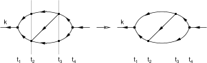
Figure 4: Unlabeled diagram on the left is converted into an unlabeled diagram without two-leg vertices corresponding to $(2\pi)^{3}\delta$ functions which is showed on the right.

For more complicated diagrams after integrating over $\delta$ functions we are still left with explicit, specific time ordering of vertices. For example, for diagrams showed in Fig. 5

Figure 5: Time ordered diagrams corresponding to different time orderings of vertices can be re-summed to give one time-unordered diagram.

we have $t_{1}\geq t_{2}\geq t_{3}\geq t_{4}$ for the first diagram, $t_{1}\geq t_{3}\geq t_{2}\geq t_{4}$ for the second, etc. We can, however, sum all such diagrams and obtain a time-unordered diagram for which there is no restriction on the ordering of times associated with different vertices (note that there is always an implicit restriction due to vanishing of response functions for $t<0$ and thus in the above example $t_{1}\geq t_{3}$ and $t_{2}\geq t_{4}$). As a result we obtain a series involving so-called time-unordered diagrams. One should note that both integrating over $\delta$ functions and replacing sums of time-ordered diagrams by time-unordered ones do not change the symmetry numbers of diagrams. In the following we implicitly assume that these transformations have been performed on all diagrams. Thus, from now on, we will consider time-unordered diagrams without $(2\pi)^{3}\delta$ vertices.

The final result of this section is the following diagrammatic expression for the response function:

$$G(k;t)=$$ (68)

sum of all topologically different diagrams with

a left root labeled $$k G_{0} \mathcal{V}_{12}$$, a right root, bonds, ,

$$\mathcal{V}_{21} \mathcal{V}_{22}$$ and vertices, in which diagrams with odd

and even numbers of $$\mathcal{V}_{22}$$ vertices contribute with

overall negative and positive sign, respectively.

VI Memory functions: reducible and irreducible

We start with the Dyson equation

$$G(k;t) = G_{0}(k;t)+\int dt_{1}dt_{2}\int\frac{d\mathbf{k}_{1}}{(2\pi)^{3}}G_{0}(k;t-t_{1})$$ (69)

$$\times\Sigma(\mathbf{k},\mathbf{k}_{1};t_{1}-t_{2})G(k_{1};t_{2}),$$

where $\Sigma$ is the self energy. Diagrammatic representation of the Dyson equation is showed in Fig. 6. Due to the translational invariance the self-energy is diagonal in wavevector,

$$\Sigma(\mathbf{k},\mathbf{k}_{1};t)\propto(2\pi)^{3}\delta(\mathbf{k}-\mathbf{k}_{1}).$$ (70)

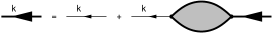
Figure 6: Diagrammatic representation of the Dyson equation, Eq. (69).

It follows from general analysis of the Dyson equation that the self-energy $\Sigma$ is a sum of diagrams that do not separate into disconnected components upon removal of a single bond.

The memory function can be obtain from $\Sigma$ in the following way. We note that the diagrams contributing to the self-energy start with $\mathcal{V}_{21}$ vertex on the right and end with $\mathcal{V}_{12}$ vertex on the left. Customarily, to define the memory function for a Brownian system one factors out parts of these vertices. First, we define memory matrix $\mathbf{M}$ by factoring out $\mathbf{k}$ from the left vertex and $(D_{0}/S(k_{1}))\mathbf{k}_{1}$ from the right vertex,

$$\Sigma(\mathbf{k},\mathbf{k}_{1};t)=D_{0}\mathbf{k}\cdot\mathbf{M}(\mathbf{k},\mathbf{k}_{1};t)\cdot\mathbf{k}_{1}S(k_{1})^{-1}.$$ (71)

Due to the translational and rotational invariance $\mathbf{M}$ is diagonal in the wavevector and longitudinal. Thus we can define memory function $M$ through the following relation

$$\mathbf{M}(\mathbf{k},\mathbf{k}_{1};t)=M(k;t)\hat{\mathbf{k}}\hat{\mathbf{k}}(2\pi)^{3}\delta(\mathbf{k}-\mathbf{k}_{1}).$$ (72)

Using Eq. (71) and (72) we can obtain the following equation from the Laplace transform of the Dyson equation,

$$G(k;z)=G_{0}(k;z)+G_{0}(k;z)\frac{D_{0}k^{2}}{S(k)}M(k;z)G(k;z).$$ (73)

Eq. (73) can be solved w.r.t. response function $G(k;z)$. Using the definition of bare response function $G_{0}$ we obtain

$$G(k;z)=\frac{1}{z+\frac{D_{0}k^{2}}{S(k)}\left(1-M(k;z)\right)}.$$ (74)

Multiplying both sides of the above equation by the static structure factor and noting that $S(k)G(k;z)=F(k;z)$, where $F$ is the collective intermediate scattering function, we get the well-known memory function representationHK of $F(k;z)$,

$$F(k;z)=\frac{S(k)}{z+\frac{D_{0}k^{2}}{S(k)}\left(1-M(k;z)\right)}.$$ (75)

To facilitate further discussion it is convenient to introduce cut-out vertices corresponding to the following functions:

$$\mathbf{V}_{12}^{c}(\mathbf{k}_{1};\mathbf{k}_{2},\mathbf{k}_{3}) = D_{0}(2\pi)^{3}\delta(\mathbf{k}_{1}-\mathbf{k}_{2}-\mathbf{k}_{3})$$ (76)

$$\times\left(c(k_{2})\mathbf{k}_{2}+c(k_{3})\mathbf{k}_{3}\right)$$

$$\mathbf{V}_{21}^{c}(\mathbf{k}_{1},\mathbf{k}_{2};\mathbf{k}_{3}) = n(2\pi)^{3}\delta(\mathbf{k}_{1}+\mathbf{k}_{2}-\mathbf{k}_{3})S(k_{1})S(k_{2})$$ (77)

$$\times\left(c(k_{1})\mathbf{k}_{1}+c(k_{2})\mathbf{k}_{2}\right).$$

These vertices are obtained by factoring out $\mathbf{k}_{1}$ from vertex $\mathcal{V}_{12}$ and $(D_{0}/S(k_{3}))\mathbf{k}_{3}$ from vertex $\mathcal{V}_{21}$.

It should be noted that

$$\mathcal{V}_{22}(\mathbf{k}_{1},\mathbf{k}_{2};\mathbf{k}_{3},\mathbf{k}_{4})$$

$$=\int\frac{d\mathbf{k}^{\prime}}{(2\pi)^{3}}\mathbf{V}_{21}^{c}(\mathbf{k}_{1},\mathbf{k}_{2};\mathbf{k}^{\prime})\cdot\mathbf{V}_{12}^{c}(\mathbf{k}^{\prime};\mathbf{k}_{3},\mathbf{k}_{4}).$$ (78)

The diagrammatic rules for functions $\mathbf{V}_{12}^{c}$ and $\mathbf{V}_{21}^{c}$ are as follows:

• “left” cut-out vertex $\mathbf{V}_{12}^{c}$:

• “right” cut-out vertex $\mathbf{V}_{21}^{c}$:

and we refer to wavevector $\mathbf{k}_{1}$ in $\mathbf{V}_{12}^{c}(\mathbf{k}_{1};\mathbf{k}_{2},\mathbf{k}_{3})$ and $\mathbf{k}_{3}$ in $\mathbf{V}_{21}^{c}(\mathbf{k}_{1},\mathbf{k}_{2};\mathbf{k}_{3})$ as roots of these vertices.

It follows from the definition of the memory matrix $\mathbf{M}$ that

$$\mathbf{M}(\mathbf{k},\mathbf{k}_{1};t)=$$ (79)

sum of all topologically different diagrams which

do not separate into disconnected components

upon removal of a single bond, with vertex $$\mathbf{V}_{12}^{c}$$

with root $$\mathbf{k} \mathbf{V}_{21}^{c} \mathbf{k}_{1}$$ on the left and vertex with root

on the right, $$G_{0} \mathcal{V}_{12} \mathcal{V}_{21} \mathcal{V}_{22}$$ bonds, , and vertices,

in which diagrams without and even numbers of $$\mathcal{V}_{22}$$

vertices contribute with overall negative and

positive sign, respectively.

The first few diagrams in the series for $\mathbf{M}$ are showed in Fig. 7.

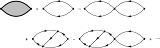
Figure 7: The first few diagrams in series expansion for memory matrix $\mathbf{M}$.

Now, one can understand the need for an irreducible memory function CHess . The series expansion for $\mathbf{M}$ consists of diagrams that are one-propagator irreducible (i.e. diagrams that do not separate into disconnected components upon removal of a single bond) but not all of these diagrams are completely one-particle irreducible. Some of the diagrams contributing to $\mathbf{M}$ separate into disconnected components upon removal of $\mathcal{V}_{22}$ vertex (and bonds attached to this vertex). The examples of such diagrams are the second and the fourth diagrams on the right-hand-side of the equality sign in Fig. 7.

We define the irreducible memory matrix $\mathbf{M}^{irr}$ as a sum of only those diagrams in the series for $\mathbf{M}$ that do not separate into disconnected components upon removal of a single $\mathcal{V}_{22}$ vertex. Diagrammatically, we can represent memory matrix $\mathbf{M}$ as a sum of $\mathbf{M}^{irr}$ and all other diagrams. The latter diagrams can be re-summed as showed in Fig. 8.

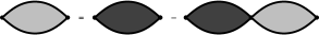
Figure 8: Memory matrix $\mathbf{M}$ can be represented as a sum of $\mathbf{M}^{irr}$ and all other diagrams. The latter diagrams can be re-summed and it is easy to see that as a result we get the second diagram at the right-hand-side.

Using Eq. (VI), we can introduce an additional integration over a wavevector and then we see that the diagrammatic equation showed in Fig. 8 corresponds to the following equation,

$$\mathbf{M}(\mathbf{k},\mathbf{k}_{1};t)=\mathbf{M}^{irr}(\mathbf{k},\mathbf{k}_{1};t)$$ (80)

$$-\int dt_{1}\int\frac{d\mathbf{k}_{2}}{(2\pi)^{3}}\mathbf{M}^{irr}(\mathbf{k},\mathbf{k}_{2};t-t_{1})\cdot\mathbf{M}(\mathbf{k}_{2},\mathbf{k}_{1};t_{2})$$

Again, we use translational and rotational invariance to introduce the irreducible memory function $M^{irr}$,

$$\mathbf{M}^{irr}(\mathbf{k},\mathbf{k}_{1};t)=M^{irr}(k;t)\hat{\mathbf{k}}\hat{\mathbf{k}}(2\pi)^{3}\delta(\mathbf{k}-\mathbf{k}_{1}),$$ (81)

Taking Laplace transform of Eq. (80) and then using Eq. (81) we obtain

$$M(k;z)=M^{irr}(k;z)-M^{irr}(k;z)M(k;z).$$ (82)

This equation can be solved w.r.t. memory function $M$. Substituting the solution into Eq. (75) we obtain a representation of the intermediate scattering function in terms of the irreducible memory function,

$$F(k;z)=S(k)G(k;z)=\frac{S(k)}{z+\frac{D_{0}k^{2}}{S(k)\left(1+M^{irr}(k;z)\right)}}.$$ (83)

Eq. (83) was first derived by Cichocki and HessCHess . It has been used as a starting point for the development of mode-coupling approximations for both equilibrium SL and driven Brownian systems FC .

Diagrammatically,

$$\mathbf{M}(\mathbf{k},\mathbf{k}_{1};t)=$$ (84)

sum of all topologically different diagrams which

do not separate into disconnected components

upon removal of a single bond or a single $$\mathcal{V}_{22}$$

vertex, with vertex $$\mathbf{V}_{12}^{c} \mathbf{k}$$ with root on the left

and vertex $$\mathbf{V}_{21}^{c} \mathbf{k}_{1} G_{0}$$ with root on the right, bonds,

$$\mathcal{V}_{12} \mathcal{V}_{21} \mathcal{V}_{22}$$, and vertices, in which diagrams with

odd and even numbers of $$\mathcal{V}_{22}$$ vertices contribute

with overall negative and positive sign, respectively.

The first few diagrams in the series for $\mathbf{M}^{irr}$ are showed in Fig. 9.

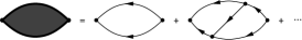
Figure 9: The first few diagrams in series expansion for irreducible memory matrix $\mathbf{M}^{irr}$.

VII Mode-coupling approximation

The simplest re-summation of the series (84) includes diagrams that separate into two disconnected components upon removal of the $\mathbf{V}_{12}^{c}$ and $\mathbf{V}_{21}^{c}$ vertices. It is easy to see that in such diagrams each of these components is a part of the series for the response function $G$. Summing all such diagrams we get a one-loop diagram (i.e. the first diagram showed on the right-hand-side in Fig. 9) but with $G_{0}$ bonds replaced by $G$ bonds, see Fig. 10.

Figure 10: Re-summation of diagrams that separate into two disconnected components upon removal of the $\mathbf{V}_{12}^{c}$ and $\mathbf{V}_{21}^{c}$ vertices leads to a one-loop diagram with $G$ bonds.

As a result of this re-summation we get one-loop self-consistent approximation for the memory matrix,

$$\mathbf{M}^{irr}_{one-loop}(\mathbf{k},\mathbf{k}_{1};t) = \int\frac{d\mathbf{k}_{2}d\mathbf{k}_{3}}{2(2\pi)^{6}}\mathbf{V}_{12}^{c}(\mathbf{k};\mathbf{k}_{2},\mathbf{k}_{3})$$

$$\times G(k_{2};t)G(k_{3};t)\mathbf{V}_{21}^{c}(\mathbf{k}_{2},\mathbf{k}_{3};\mathbf{k}_{1}).$$

The factor 2 in the denominator is the symmetry number of the single-loop diagram.

Using explicit expressions (76-77) for the cut-out vertices we easily show that (VII) leads to the following expression for the irreducible memory function

$$M^{irr}_{one-loop}(k;t)=$$

$$\frac{nD_{0}}{2}\int\frac{d\mathbf{k}_{1}}{(2\pi)^{3}}\left(c(k_{1})\hat{\mathbf{k}}\cdot\mathbf{k}_{1}+c(|\mathbf{k}-\mathbf{k}_{1}|)\hat{\mathbf{k}}\cdot(\mathbf{k}-\mathbf{k}_{1})\right)^{2}$$

$$\times S(k_{1})S(|\mathbf{k}-\mathbf{k}_{1}|)G(k_{1};t)G(|\mathbf{k}-\mathbf{k}_{1}|;t)\equiv M^{irr}_{MCT}(k;t)$$

As indicated above, the one-loop self-consistent approximation coincides with the mode-coupling approximation, i.e. both approximations result in exactly the same expression for the irreducible memory function.

Expression (VII) was first derived using a projection operator approach SL . Subsequently, it was also derived using a field theory version KM of a dynamic density functional theory of Kawasaki Kawasaki . Later, it was noticed field1 that the latter derivation was incompatible with the fluctuation-dissipation theorem. Recently, there appeared two new field-theoretical derivations of the mode-coupling theory for Brownian systems field2 ; field3 . Only one of these derivations field3 leads to expression (VII) that was originally derived using projection operator method. The other derivation field2 results in a equation that has the same structure as (VII) but involves different vertices.

VIII Discussion

We have presented a diagrammatic formulation of a theory for the time dependence of density fluctuations in equilibrium systems of interacting Brownian particles. We have analyzed the series expansion for the time-dependent response function and have obtained diagrammatic expressions for both the memory function and the irreducible memory function. The one-loop self-consistent approximation for the latter function coincides with the mode-coupling expression derived via the projection operator method.

To derive a diagrammatic expansion for the time-dependent response function we have neglected contributions to the vertices from higher-order terms in the cluster expansion. It should be noticed that in spite of this fact we obtained the same mode-coupling expression as the one derived using the projection operator method. This suggests that the diagrammatic series (68) contains all the dynamical events that result in the standard mode-coupling approximation. It would be interesting to use series (68) as a starting point for the development of theories that go beyond the standard mode-coupling approximation, i.e. to include at least some classes of the diagrams that are neglected in the one-loop re-summation. Also, it would be interesting to investigate diagrammatic interpretation of so-called generalized mode-coupling theories gMCT . Finally, the formalism presented here could be used to derive an approximate theory for the time-dependence of various four-point correlation functions. Such functions have been extensively studied in the last decade four . They provide quantitative information about so-called dynamic heterogeneity or, more precisely, about correlations of dynamics of different particles.

One of the consequences of neglecting the contributions to the vertices from higher-order terms in the cluster expansion is that the approximate equations of motion (IV-59) do not reproduce the exact short-time behavior of the density correlation function. In addition, as noted by Andersen H3 , on physical grounds one would expect that in the mode-coupling formula (VII) the vertices are replaced by matrix elements of a binary collision operator. We plan to rectify these two drawbacks of the present approach in future work.

The advantage of the present approach is that it leads to a relatively simple diagrammatic series. Thus, it should be possible to derive a field theoretical representation of this series. We note, however, that our diagrammatic series is different from series expansions that have been derived from various field theoretical approaches field1 ; field2 ; field3 ; RC . First, our series involves one dynamical function whereas field-theoretical expansions are typically formulated in terms of two functions, a correlation function and a response function (that is different from the response function used in our formalism). In addition, series (68) involves both three- and four-leg vertices whereas series expansions resulting from field theoretical approaches typically involve only three-leg vertices. Finally, in our series the renormalization of bare interactions occurs naturally. In field theoretical approaches one either carries bare interactions throughout or one has to start from a phenomenological formulation of dynamics that involves the direct correlation function.

References

• (1) See, e.g., K.S. Schweizer and E.J. Saltzman, J. Chem. Phys. 119, 1181 (2003); K. Kroy, M.E. Cates, and W.C.K. Poon, Phys. Rev. Lett. 92, 148302 (2004); J. Wu and J. Cao, Phys. Rev. Lett. 95 078301 (2005); K.S. Schweizer, J. Chem. Phys. 123, 244501 (2005); J.M. Brader, Th. Voigtmann, M.E. Cates, and M. Fuchs, Phys. Rev. Lett. 98, 058301 (2007).
• (2) For a general introduction see J.K.G. Dhont, An Introduction to Dynamics of Colloids (Elsevier, New York, 1996).
• (3) See, e.g., R. Besseling et al., arXiv:cond-mat/0605247v3; C.R. Nugent, H.N. Patel, and E.R. Weeks, arXiv:cond-mat/0601648v1; for a recent review see L. Cipelletti and L. Ramos, J. Phys. Cond. Matter 17 R253 (2005).
• (4) H.C. Andersen, J. Phys. Chem. B 106, 8326 (2002).
• (5) H.C. Andersen, J. Phys. Chem. B 107, 10226 (2003).
• (6) H.C. Andersen, J. Phys. Chem. B 107, 10234 (2003).
• (7) C.D. Boley, Phys. Rev. A 11, 328 (1975).
• (8) It should be mentioned here that a related orthogonal basis was used by J. Schofield, R. Lim and I. Oppenheim [Physica A 181, 89 (1992)] in their derivation of a general hydrodynamic mode-coupling theory; this theory was later analyzed by C.Z.-W. Liu and I. Oppenheim [Physica A 247, 183 (1997)].
• (9) K. Miyazaki and D. Reichman, J. Phys. A 38, L343 (2005).
• (10) A. Andreanov, G. Biroli, and A. Lefevre, J. Stat. Mech. P07008 (2006).
• (11) B. Kim and K. Kawasaki, J. Phys. A 40, F33 (2007).
• (12) A. Andreanov et al., Phys. Rev. E 74, 030101(R) (2006).
• (13) W. Götze, in Liquids, Freezing and Glass Transition, J.P. Hansen, D. Levesque, and J. Zinn-Justin, eds. (North-Holland, Amsterdam, 1991).
• (14) For a derivation for a colloidal system see G. Szamel and H. Löwen, Phys. Rev. A 44, 8215 (1991).
• (15) K. Kawasaki and S. Miyazima, Z. Phys. B 103 423 (1997).
• (16) N.V. Prokofev and B.V. Svistunov, Phys. Rev. Lett. 81, 2514 (1998).
• (17) M. Berciu, Phys. Rev. Lett. 97, 036402 (2006); G.L. Goodvin, M. Berciu, and G.A. Sawatzky, Phys. Rev. B 74, 245101 (2006).
• (18) G. Szamel and J. A. Leegwater, Phys. Rev. A 46, 5012 (1992).
• (19) G. Szamel, Europhys. Lett. 65, 498 (2004).
• (20) H.C. Andersen, in Statistical Mechanics, Part A: Equilibrium Techniques, B.J. Berne, ed. (Plenum, New York, 1977); J.-P. Hansen and I.R. McDonald, Theory of Simple Liquids, (Academic, London, 1986).
• (21) W. Hess and R. Klein, Adv. Phys. 32, 173 (1983).
• (22) B. Cichocki and W. Hess, Physica A 141, 475 (1987).
• (23) M. Fuchs and M.E. Cates, Phys. Rev. Lett. 89, 248304 (2002).
• (24) K. Kawasaki, Physica A 208, 35 (1994).
• (25) G. Szamel, Phys. Rev. Lett. 90, 228301 (2003); P. Mayer, K. Miyazaki, and D.R. Reichman, Phys. Rev. Lett. 97, 095702 (2006).
• (26) See, e.g., S.C. Glotzer, V.N. Novikov, and T.B. Schrøder, J. Chem. Phys. 112, 509 (2000); N. Lac̆ević et al., J. Chem. Phys. 119, 7372 (2003); G. Biroli and J.-P. Bouchaud, Europhys. Lett. 67, 21 (2004); L. Berthier et al., J. Chem. Phys. 126, 184503 (2007); L. Berthier et al., J. Chem. Phys. 126, 184504 (2007).
• (27) For a review see, e.g., D.R. Reichman and P. Charbonneau, J. Stat. Mech. P05013 (2005).