SPhT-T07/059

Bubbles on Manifolds with a $U(1)$ Isometry

Iosif Bena¹, Nikolay Bobev² and Nicholas P. Warner²

¹ Service de Physique Théorique,

CEA Saclay, 91191 Gif sur Yvette, France

² Department of Physics and Astronomy

University of Southern California

Los Angeles, CA 90089, USA

iosif.bena@cea.fr, bobev@usc.edu, warner@usc.edu

We investigate the construction of five-dimensional, three-charge supergravity solutions that only have a rotational $U(1)$ isometry. We show that such solutions can be obtained as warped compactifications with a singular ambi-polar hyper-Kähler base space and singular warp factors. We show that the complete solution is regular around the critical surface of the ambi-polar base. We illustrate this by presenting the explicit form of the most general supersymmetric solutions that can be obtained from an Atiyah-Hitchin base space and its ambi-polar generalizations. We make a parallel analysis using an ambi-polar generalization of the Eguchi-Hanson base space metric. We also show how the bubbling procedure applied to the ambi-polar Eguchi-Hanson metric can convert it to a global $AdS_{2}\times S^{3}$ compactification.

1 Introduction

Geometric transitions have proven to be an essential part of understanding string theory and strongly coupled quantum field theories. It has also become evident that such transitions will play a central role in understanding the geometry of microstates of the three-charge black hole or black ring in five dimensions. Indeed, one can argue [1] that a very large number of horizonless three-charge brane configurations, when brought to strong effective coupling, undergo a geometric transition and become smooth horizonless geometries with black-hole or black-ring charges. The black hole and black ring charges come entirely from fluxes wrapping topologically non-trivial cycles, or bubbles. All these “bubbling black hole” geometries are dual to states of the conformal field theory describing the three-charge black hole, and their physics strongly supports the idea that black holes in string theory are not fundamental objects, but rather effective thermodynamic descriptions of a huge number of horizonless configurations (see [2, 3] for a review).

The simplest starting point for the construction of three-charge geometries is M-theory, where one takes the eleven-dimensional supersymmetric metrics to have the form [4, 5]:

$$ds_{11}^{2}=ds_{5}^{2} + \left(Z_{2}Z_{3}Z_{1}^{-2}\right)^{1\over 3}(dx_{5}^{2}+dx_{6}^{2})$$ (1.1)

$$+ \left(Z_{1}Z_{3}Z_{2}^{-2}\right)^{1\over 3}(dx_{7}^{2}+dx_{8}^{2})+\left(Z_{1}Z_{2}Z_{3}^{-2}\right)^{1\over 3}(dx_{9}^{2}+dx_{10}^{2})\,.$$

The six coordinates, $x_{A}$, parameterize the compactification torus, $T^{6}$, and the five-dimensional space-time metric has the form:

$$ds_{5}^{2}~{}\equiv~{}-\left(Z_{1}Z_{2}Z_{3}\right)^{-{2\over 3}}(dt+k)^{2}+\left(Z_{1}Z_{2}Z_{3}\right)^{1\over 3}\,ds_{4}^{2}\,.$$ (1.2)

When constructing black-hole or black-ring solutions [6, 7, 4, 8, 12], the spatial “base metric,” $ds_{4}^{2}$, is usually taken to be that of flat $\mathbb{R}^{4}$, however supersymmetry is preserved if one has any hyper-Kähler metric on the the base [9].

To construct bubbling solutions corresponding to five-dimensional black holes and black rings, the asymptotic structure of $ds_{4}^{2}$ must still be that of $\mathbb{R}^{4}$ and the conventional wisdom suggested that this implies that the hyper-Kähler base metric must be flat $\mathbb{R}^{4}$, globally. The breakthrough came via [10, 1, 11], where it was realized that the base metric could be “ambi-polar,” that is, it could change its overall signature from $(+,+,+,+)$ to $(-,-,-,-)$ in some regions. The warp factors, $Z_{I}$, are also singular and change sign, but the complete five-dimensional (or eleven-dimensional) solution is still a physical, Lorentzian metric. This opens up a vast number of new possibilities for constructing bubbling black holes using four-dimensional hyper-Kähler base metrics.

The construction of the most general solutions proceeds in several steps using the linear system of “BPS equations” [4]. One first chooses the ambi-polar, hyper-Kähler base metric. This base will generically have non-trivial two-cycles (“bubbles”) with moduli that determine the size and orientation of the cycles. Dual to these bubbles are normalizable, self-dual, harmonic two-forms (the compact cohomology). There are also three non-normalizable, anti-self-dual, harmonic two-forms and these correspond to the three complex structures of the hyper-Kähler base. The normalizable harmonic two-forms determine the electromagnetic fluxes, which in turn source the warp factors, $Z_{I}$. Finally, the warp factors and the fluxes combine to give the source in the linear equation for the angular momentum vector, $k$, in (1.2).

This procedure is easiest implemented when one considers ambi-polar Gibbons-Hawking (GH) metrics, which are hyper-Kähler metrics with a tri-holomorphic $U(1)$ symmetry. All five-dimensional, supersymmetric solutions with Gibbons-Hawking base can be written in terms of several harmonic functions [9, 12, 13]; choosing an ambi-polar GH metric (with positive and negative GH charges) and specific harmonic functions ensures that the resulting “bubbling” solutions are horizonless, smooth, and have black hole and black ring charges [1, 11, 14, 15, 16, 17, 18].

At the last step of the construction, some of the moduli of the bubbles have to be fixed so as to remove closed time-like curves (CTC’s). This step has a simple, physical interpretation: The ambi-polar base metric typically arises because one has used both positive and negative geometric charges (e.g. GH charges) that tend to attract one another and would cause the space to collapse if they were not stabilized in some manner. If one seeks BPS solutions without including any physical stabilizing mechanism, the instability will manifest itself through the appearance of closed time-like curves (CTC’s). On the other hand, a flux threading a cycle tends to cause that cycle to expand. Hence, by distributing fluxes on the space one can balance the attraction of the geometric charges against the expansion caused by fluxes. The bubbles thus settle down at a size where the attractive and expansion forces cancel and the result is a stable BPS solution free of CTC’s. One generically finds that the sizes of the bubbles are set in terms of the fluxes threading them. Other bubble moduli, like orientations, remain free. The equations that express this balance of fluxes and bubble sizes are called the “bubble equations” [1, 11].

Studying solutions that have an ambi-polar Gibbons-Hawking base has quite a few advantages: the construction of these solutions is straightforward, the solutions can be related to four-dimensional, multi-centered “D6 - $\overline{\rm D6}$” solutions [19, 13, 20] , they can arise from the geometric transition of circular three-charge supertubes [21, 1], and they can describe microstates both of zero-entropy black holes and black rings [15], or of black holes and black rings with macroscopic horizons [16, 22].

Despite the remarkable results that have been obtained using Gibbons-Hawking geometries, such metrics represent a major restriction. In particular, they all have a translational (tri-holomorphic) $U(1)$ isometry [24], which is a combination of the two $U(1)$’s in the $\mathbb{R}^{2}$ planes that make up the $\mathbb{R}^{4}$ in the asymptotic region. Thus, bubbling solutions with a GH base cannot capture quite a host of interesting physical processes that do not respect this symmetry, like the merger of two BMPV black holes, or the geometric transition of a three-charge supertube of arbitrary shape. In [1] it was argued that this geometric transition results in bubbling solutions that have an ambi-polar hyper-Kähler base, and that depend on a very large number of arbitrary continuous functions. Counting these solutions is a way to prove the general conjecture that black holes are ensembles of smooth horizonless configurations. It is therefore of great interest to construct and understand them.

In this paper we will take a step in this direction by considering such metrics that also have a general $U(1)$ isometry. These metrics are much less restrictive than GH-based metrics. Moreover, they could also arise from the geometric transition of supertubes that preserve a rotational $U(1)$, and hence could also depend on an arbitrarily large number of continuous functions. Constructing and counting such solutions is also of interest in the program to prove that black holes are ensembles of smooth horizonless configurations. Even if the entropy in these symmetric configurations will be smaller than the entropy of the black hole, it might give some insight into the structure and charge dependence of the most general, non-symmetric configuration.

An important feature of all bubbled solutions is that the ambi-polar base space and the fluxes dual to the homology are singular on the critical surfaces where the metric changes sign. For ambi-polar GH spaces it was possible to use the explicit solutions to show that all these singularities were canceled and the final result was a regular, five-dimensional space-time background in M-theory. Our analysis here will illustrate how this happens for the general $U(1)$-invariant bubbled background, and this work suggests that the most general bubbling geometries will have also this property.

Before beginning, we would like to stress that constructing solutions that only have a rotational $U(1)$ is a rather tedious and challenging task. For classical black holes and black rings, only two such solutions exist: one describing a black ring with an arbitrary charge density [25], and one describing a black ring with a black hole away from the center of the ring [26]. In this paper we will succeed in constructing the first explicit bubbling solution in this class, using a base that is a generalization of the Atiyah-Hitchin metric. Nevertheless, the most general bubbling solutions that only have a rotational $U(1)$ invariance will be much more complicated, and perhaps even impossible to write down explicitly.

2 Prelude

It has been known for a long time that hyper-Kähler metrics with a generic (rotational) $U(1)$ isometry can be obtained by solving the $SU(\infty)$ Toda equation [27, 28, 29]. The coordinates can be chosen so that the metric takes the form:

$$ds^{2}_{4}~{}=~{}V^{-1}\,(d\tau+A_{i}dx^{i})^{2}~{}+~{}V\gamma_{ij}\,dx^{i}dx^{j}\,,$$ (2.3)

with $\gamma_{ij}=0$ for $i\neq j$ and

$$\gamma_{11}~{}=~{}\gamma_{22}~{}=~{}e^{\nu}\,,\qquad\gamma_{33}~{}=~{}1\,,$$ (2.4)

for some function, $\nu$. The function, $V$, and the vector field, $A$, are given by

$$V~{}=~{}\partial_{z}\nu\,,\qquad A_{1}~{}=~{}\partial_{y}\nu\,,\qquad A_{2}~{}=~{}-\partial_{x}\nu\,,\qquad A_{3}~{}=~{}0\,,$$ (2.5)

and the function $\nu$ must satisfy:

$$\partial_{x}^{2}\,\nu~{}+~{}\partial_{y}^{2}\,\nu~{}+~{}\partial_{z}^{2}\,(e^{\nu})~{}=~{}0\,.$$ (2.6)

This equation is called the $SU(\infty)$ Toda equation, and may be viewed as a continuum limit of the $SU(N)$ Toda equation. Even though the $SU(\infty)$ Toda equation is integrable, surprisingly little is know about its solutions, and there appears to be no known analog of the known soliton solutions of the $SU(N)$ Toda equation. On the other hand, the metric is determined in terms of a single function and (2.3) is a relatively mild generalization of the Gibbons-Hawking metrics.

Our purpose here is to construct three-charge solutions based upon ambi-polar hyper-Kähler metrics with generic (non-tri-holomorphic) $U(1)$ isometries. We will do this in two different ways, first by building such solutions using a general metric of the form (2.3) on the base space. We will then consider the Atiyah-Hitchin metric: This metric has an $SO(3)$ isometry, but none of the $U(1)$ subgroups is tri-holomorphic. Just as with the GH metric, the metric (2.3), is ambi-polar if we allow $V=\partial_{z}\nu$ to change sign. Thus the primary issue of regularity in the five-dimensional metric arises on the critical surfaces where $V=0$. While we will not be able to construct general solutions as explicitly as can be done for GH metrics, we will show that the five-dimensional metric is regular and Lorentzian in the neighborhood of these critical surfaces.

The standard Atiyah-Hitchin metric [30] arises as the solution of a first order, non-linear Darboux-Halphen system for the three metric coefficient functions. This system is analytically solvable in terms of the solution of a single, second order linear differential equation. Indeed, the solutions of the latter equation are expressible in terms of elliptic functions. The standard practice is to choose the solution of this linear equation so that the metric functions are regular, and the result is a smooth geometry that closes off at a non-trivial “bolt,” or two-cycle in the center. We will show that if one selects the most general solution of the linear differential equation, then one obtains an ambi-polar generalization of the Atiyah-Hitchin metric. Moreover, one can set up regular, cohomological fluxes on the two-cycle and the resulting warp factors render the five-dimensional metric perfectly smooth and regular across the critical surface.

The ambi-polar Atiyah-Hitchin metric actually continues through the bolt and initially appears to have two regions, one on each side of the bolt, that are asymptotic to $\mathbb{R}^{3}\times S^{1}$. It thus looks like a wormhole. Unfortunately, the solution cannot be made regular on both its asymptotic regions. Indeed, upon imposing asymtotic flatness on one side of the wormhole, one finds that the warp factors change sign twice, once on the critical surface and again as one enters one of the asymptotic regions. Thus the critical surface is regular, but there is another potentially singular region elsewhere. However, we find that if we tune the flux through the bubble to exactly the proper value, one can pinch off the metric just as the warp factors change sign for the second time. The result is a Lorentzian metric, that extends smoothly through the critical surface ($V=0$). The pinching off of the metric does however result in a curvature singularity that is very similar to the one encountered in the Klebanov-Tseytlin solution [31]. We will argue that the singularity of our new, non-trivial BPS solution is also a consequence of the very high level of symmetry, and that it will be resolved via a mechanism similar to that in [32].

We also consider solutions based upon an ambi-polar generalization of the Eguchi-Hanson metric, obtained by making an analytic continuation of the standard Eguchi-Hanson metric, and extending the range of one of the coordinates. The singular structure of this metric is precisely what is needed to render it ambi-polar. Hence, upon adding fluxes and warp factors this metric gives us regular five-dimensional solutions that have similar features to the bubling Atiyah-Hitchin solution. There is also one surprise: One of the Eguchi-Hanson “wormhole” solutions is completely regular everywhere and is nothing other than the global $AdS_{2}\times S^{3}$ Robinson-Bertotti solution.

In Section 3 we will review the BPS equations and discuss their solution for a metric with a generic $U(1)$ isometry. In Section 4 we will review the properties and structure of the Atiyah-Hitchin metric. Section 5 is devoted to the explicit solution of the system of BPS equations for the Atiyah-Hitchin metric and its ambi-polar generalization, and a discussion on regularity and CTC’s. In Section 6 we present the bubbled solutions on the generalized (ambi-polar) Eguchi-Hanson background and we show how they closely parallel the results for the generalized (ambi-polar) Atiyah-Hitchin solution. We also show how to obtain global $AdS_{2}\times S^{3}$ as a bubbling Eguchi-Hanson solution. Finally, Section 7 contains our conclusions and a discussion of possible future work.

3 The general $U(1)$ invariant geometries

3.1 The BPS equations

The supersymmetric, BPS solutions to M-theory with metric given by (1.1) have Maxwell three-form potential given by:

$$C^{(3)}=A^{(1)}\wedge dx_{5}\wedge dx_{6}~{}+~{}A^{(2)}\wedge dx_{7}\wedge dx_{8}~{}+~{}A^{(3)}\wedge dx_{9}\wedge dx_{10}\,,$$ (3.7)

where the $A^{(I)}$, $I=1,2,3$, are one-form Maxwell potentials in the five-dimensional space-time and depend only upon the coordinates, $y^{\mu}$, $\mu=1,\dots,4$, that parameterize the spatial directions of $ds_{4}$. It is convenient to introduce the Maxwell “dipole field strengths,” $\Theta^{(I)}$, obtained by removing the contributions of the electrostatic potentials:

$$\Theta^{(I)}~{}\equiv~{}dA^{(I)}+d\big{(}Z_{I}^{-1}\,(dt+k)\big{)}\,.$$ (3.8)

The most general supersymmetric configuration is then obtained by solving the BPS equations:

$$\Theta^{(I)} ~{}=~{} \star_{4}\,\Theta^{(I)}\,,$$ (3.9)

$$\nabla^{2}Z_{I} ~{}=~{} {1\over 2}C_{IJK}\star_{4}(\Theta^{(J)}\wedge\Theta^{(K)})\,,$$ (3.10)

$$dk~{}+~{}\star_{4}dk ~{}=~{} Z_{I}\,\Theta^{(I)}\,,$$ (3.11)

where $\star_{4}$ is the Hodge dual taken with respect to the four-dimensional base metric, $ds_{4}^{2}$, and for the structure constants are given by $C_{IJK}~{}\equiv~{}|\epsilon_{IJK}|$. The BPS equations generalize trivially to more general $U(1)^{N}$ five-dimensional ungauged supergravities.

The first step in solving this linear system is to identify the self-dual, harmonic two-forms, $\Theta^{(I)}$. In a Kähler manifold this is, at least theoretically, straightforward because such two-forms are related to the moduli of the metric. For a hyper-Kähler metric there are three complex structures, $J_{(i)}$, $i=1,2,3$, and given a harmonic two-form, $\omega$, one can define three symmetric tensors via:

$$h^{(i)}_{\mu\nu}~{}\equiv~{}{J_{(i)\,\mu}}^{\rho}\,\omega_{\rho\nu}~{}-~{}{J_{(i)\,\nu}}^{\rho}\,\omega_{\mu\rho}\,.$$ (3.12)

These tensors may be viewed as metric perturbations and as such they represent perturbations that preserve the hyper-Kähler structure. In particular, they are zero modes of the Lichnerowicz operator.

For the metric (2.3) it is convenient to introduce vierbeins:

$$\hat{e}^{1}=V^{-1/2}(d\tau+A_{i}dx^{i})\,,\qquad\hat{e}^{2}=V^{1/2}e^{\nu/2}dx\,,\qquad\hat{e}^{3}=V^{1/2}e^{\nu/2}dy\,,\qquad\hat{e}^{4}=V^{1/2}dz\,,$$ (3.13)

and introduce a basis for the self-dual and anti-self dual two forms:

$$\Omega_{\pm}^{(1)} = (d\tau+A_{2}dy)\wedge dx~{}\pm~{}Vdy\wedge dz~{}=~{}e^{-\nu/2}(\hat{e}^{1}\wedge\hat{e}^{2}~{}\pm~{}\hat{e}^{3}\wedge\hat{e}^{4})\,,$$ (3.14)

$$\Omega_{\pm}^{(2)} = (d\tau+A_{1}dx)\wedge dy~{}\pm~{}Vdz\wedge dx~{}=~{}e^{-\nu/2}(\hat{e}^{1}\wedge\hat{e}^{3}~{}\pm~{}\hat{e}^{4}\wedge\hat{e}^{2})\,,$$ (3.15)

$$\Omega_{\pm}^{(3)} = (d\tau+A_{1}dx+A_{2}dy)\wedge dz~{}\pm~{}e^{\nu}Vdx\wedge dy~{}=~{}(\hat{e}^{1}\wedge\hat{e}^{4}~{}\pm~{}\hat{e}^{2}\wedge\hat{e}^{3})\,.$$ (3.16)

The three Kähler forms are then given by [29]:

$$J_{(1)} = e^{\nu/2}\cos\Big{(}\frac{\tau}{2}\Big{)}\,\Omega_{-}^{(1)}~{}+~{}e^{\nu/2}\sin\Big{(}\frac{\tau}{2}\Big{)}\,\Omega_{-}^{(2)\,,}$$ (3.17)

$$J_{(2)} = e^{\nu/2}\sin\Big{(}\frac{\tau}{2}\Big{)}\,\Omega_{-}^{(1)}~{}-~{}e^{\nu/2}\cos\Big{(}\frac{\tau}{2}\Big{)}\Omega_{-}^{(2)}\,,$$ (3.18)

$$J_{(3)} = \Omega_{-}^{(3)}\,,$$ (3.19)

and they satisfy the proper quaternionic algebra:

$${J_{(i)\,\mu}}^{\rho}\,{J_{(j)\,\rho}}^{\nu}~{}=~{}\delta_{ij}\,\delta_{\mu}^{\nu}~{}-~{}\varepsilon_{ijk}\,{J_{(k)\,\mu}}^{\nu}\,.$$ (3.20)

Following [1], we make an Ansatz for the harmonic, self-dual field strengths, $\Theta^{(I)}$:

$$\Theta^{(I)}~{}=~{}\sum_{a=1}^{3}\partial_{a}(\dot{\nu}^{-1}K^{I})\,\Omega_{+}^{(a)}\,,$$ (3.21)

where the dot represents derivative with respect to $z$. We then find that the $K^{I}$ must satisfy the linearized Toda equation (it follows from (2.6) that $\dot{\nu}$ also solves this equation):

$${\cal L_{T}}\,K^{I}~{}\equiv~{}\partial_{x}^{2}K^{I}~{}+~{}\partial_{y}^{2}K^{I}~{}+~{}\partial_{z}^{2}(e^{\nu}K^{I})~{}=~{}0\,.$$ (3.22)

For later convenience, we note that there are relatively simple vector potentials such that $\Theta^{(I)}=dB^{(I)}$:

$$B^{(I)}~{}\equiv~{}\dot{\nu}^{-1}\,K^{I}\,(d\tau+A)~{}+~{}{\vec{\xi}}^{\,(I)}\cdot d\vec{x}\,,$$ (3.23)

where

$$(\vec{\nabla}\times{\vec{\xi}}^{\,(I)})^{j}~{}=~{}-\partial_{i}\big{(}\gamma^{ij}e^{\nu}K^{I}\big{)}\,.$$ (3.24)

Hence, ${\vec{\xi}}^{\,(I)}$ is a vector potential for magnetic monopoles located at the singular points of $K^{I}$.

Since the $K^{I}$ satisfy the linearized Toda equation, we see the direct relationship between the harmonic forms and linearized fluctuations of the metric. In practice, (3.12) and (3.21) do not yield exactly the same result as the direct substitution of fluctuations in $\nu$ into (2.3) but they are equivalent up to infinitesimal diffeomorphisms. For example, the metric fluctuation obtained from using (3.21) and $J_{(3)}$ in (3.12) is identical with the metric fluctuation, $\nu\to\nu+\epsilon K^{I}$, combined with the infinitesimal diffeomorphism, $z\to z-\epsilon\dot{\nu}^{-1}K^{I}$.

The second BPS equation reduces to:

$${\cal L}Z_{I}~{}=~{}\dot{\nu}\,e^{\nu}\,C_{IJK}\,\gamma^{ij}\partial_{i}\Big{(}{K^{J}\over\dot{\nu}}\Big{)}\,\partial_{j}\Big{(}{K^{K}\over\dot{\nu}}\Big{)}\,,$$ (3.25)

where $\gamma_{ij}$ is the three-metric in (2.4) and ${\cal L}$ is given by:

$${\cal L}\,F~{}\equiv~{}\dot{\nu}\,e^{\nu}\,\nabla_{\gamma}^{2}F~{}=~{}\partial_{x}^{2}F+~{}\partial_{y}^{2}F~{}+~{}\partial_{z}(e^{\nu}\partial_{z}F)\,.$$ (3.26)

The operator, $\nabla_{\gamma}^{2}$, denotes the Laplacian in the metric $\gamma_{ij}$.

The natural guess for the solution is to follow, once again, [1] and try:

$$Z_{I}~{}\equiv~{}{\textstyle{1\over 2}}\displaystyle\,C_{IJK}\,\dot{\nu}^{-1}\,K^{J}K^{K}~{}+~{}Z_{I}^{(0)}\,.$$ (3.27)

One then finds that $Z_{I}^{(0)}$ is not a solution of the homogeneous equation, but

$${\cal L}\,Z_{I}^{(0)}~{}=~{}-\partial_{z}\big{(}{\textstyle{1\over 2}}\displaystyle\,e^{\nu}\,C_{IJK}\,K^{J}K^{K}\big{)}\,.$$ (3.28)

Intriguingly, one can also check that:

$${\cal L}_{T}\big{(}{\textstyle{1\over 2}}\displaystyle\,C_{IJK}\,\dot{\nu}^{-1}\,K^{J}K^{K}\big{)}~{}=~{}\dot{\nu}\,e^{\nu}\,C_{IJK}\,\gamma^{ij}\partial_{i}\Big{(}{K^{J}\over\dot{\nu}}\Big{)}\,\partial_{j}\Big{(}{K^{K}\over\dot{\nu}}\Big{)}\,,$$ (3.29)

where ${\cal L}_{T}$ is the linearized Toda operator (3.22) and so one has the explicit solution but to the wrong equation.

The important point, however, is that the source on the right-hand side of (3.28) is regular as $\dot{\nu}\to 0$, and so $Z_{I}^{(0)}$ is regular on any critical surface where one has $\dot{\nu}=0$.

To solve the last BPS equation for the angular momentum vector, $k$, we make the Ansatz:

$$k~{}=~{}\mu\,(d\tau+A)~{}+~{}\omega\,,$$ (3.30)

where $\omega$ is a one form in the three-dimensional space defined by $(x,y,z)$. Define yet another linear operator:

$$\widetilde{\cal L}\,F~{}\equiv~{}e^{\nu}\gamma^{ij}\,\partial_{i}\,\partial_{j}F~{}=~{}\partial_{x}^{2}F+~{}\partial_{y}^{2}F~{}+~{}e^{\nu}\,\partial_{z}^{2}F\,,$$ (3.31)

and then one finds that $\mu$ and $\omega$ must satisfy:

$$\widetilde{\cal L}\,\mu~{}=~{}\dot{\nu}^{-1}\,\partial_{i}\Big{(}\dot{\nu}\,e^{\nu}\,\gamma^{ij}\,\sum_{I=1}^{3}\,Z_{I}\,\partial_{j}\Big{(}{K^{I}\over\dot{\nu}}\Big{)}\Big{)}\,,$$ (3.32)

and

$$(\vec{\nabla}\times\vec{\omega})^{i}~{}=~{}\dot{\nu}\,e^{\nu}\gamma^{ij}\partial_{j}\mu~{}-~{}\mu\,\partial_{j}(e^{\nu}\gamma^{ij}\dot{\nu})~{}-~{}\dot{\nu}\,e^{\nu}\,Z_{I}\,\gamma^{ij}\,\partial_{j}\Big{(}{K^{I}\over\dot{\nu}}\Big{)}\,.$$ (3.33)

Note that the integrability of the equation for $\omega$ is precisely the equation (3.32) for $\mu$, provided that one also uses the fact that $\nu$ satisfies (2.6). The structure of these equations also closely parallels those encountered for a GH base metric [1, 11].

Once again one can try a form of the solution based upon the results for GH spaces. Define $\mu_{0}$ by:

$$\mu = {\textstyle{1\over 2}}\displaystyle\,\dot{\nu}^{-1}\,Z_{I}\,K^{I}~{}-~{}{\textstyle{1\over 12}}\displaystyle\,\dot{\nu}^{-2}\,C_{IJK}\,K^{I}K^{J}K^{K}~{}+~{}\mu_{0}$$ (3.34)

$$= {\textstyle{1\over 2}}\displaystyle\,\dot{\nu}^{-1}\,Z_{I}^{(0)}\,K^{I}~{}+~{}{\textstyle{1\over 6}}\displaystyle\,\dot{\nu}^{-2}\,C_{IJK}\,K^{I}K^{J}K^{K}~{}+~{}\mu_{0}\,,$$

and one then finds that $\mu_{0}$ must satisfy:

$$\widetilde{\cal L}\,\mu_{0}~{}=~{}-{\textstyle{1\over 2}}\displaystyle\,e^{\nu}\,K^{I}\,\partial_{z}Z_{I}^{(0)}~{}+~{}{\textstyle{1\over 12}}\displaystyle\,e^{\nu}\,C_{IJK}\,K^{I}K^{J}K^{K}\,.$$ (3.35)

Again note that the source is regular as $\dot{\nu}\to 0$ and so $\mu_{0}$ will be similarly regular as $\dot{\nu}\to 0$.

Finally, if one substitutes these expressions for $Z_{I}$ and $\mu$ into (3.33), one obtains:

$$(\vec{\nabla}\times\vec{\omega})^{i} = \dot{\nu}\,e^{\nu}\gamma^{ij}\partial_{j}\mu_{0}~{}-~{}\mu_{0}\,\partial_{j}(e^{\nu}\gamma^{ij}\dot{\nu})~{}+~{}{\textstyle{1\over 2}}\displaystyle\,K^{I}\partial_{j}\big{(}e^{\nu}\gamma^{ij}Z_{I}^{(0)}\big{)}~{}-~{}{\textstyle{1\over 2}}\displaystyle\,e^{\nu}\gamma^{ij}Z_{I}^{(0)}\partial_{j}K^{I}$$ (3.36)

$$~{}-~{}{\textstyle{1\over 6}}\displaystyle\,\delta^{i}_{3}\,e^{\nu}\,C_{IJK}\,K^{I}K^{J}K^{K}\,,$$

where the $\delta^{i}_{3}$ means that the last term only appears for $i=3$. Note that $\vec{\omega}$ has sources that are regular as $\dot{\nu}\to 0$ and so $\vec{\omega}$ will be regular on critical surfaces.

Therefore, in this more general class of metrics, we cannot find the solutions to the BPS equations as explicitly as one can for GH base metrics. However, one can completely and explicitly characterize the singular parts of the solutions as one approaches critical surfaces where $\dot{\nu}\to 0$.

3.2 Regularity on the critical surfaces

Consider the behavior of the metric (1.2) as $\dot{\nu}\to 0$. The warp factors, $Z_{I}$ diverge as $\dot{\nu}^{-1}$, $\mu$ diverges as $\dot{\nu}^{-2}$ and so the only potentially divergent part of the metric is:

$$-\big{(}Z_{1}Z_{2}Z_{3}\big{)}^{-{2\over 3}}\mu^{2}(d\tau+A)^{2}+\big{(}Z_{1}Z_{2}Z_{3}\big{)}^{1\over 3}\,\dot{\nu}^{-1}\,(d\tau+A)^{2}~{}=~{}\big{(}Z_{1}Z_{2}Z_{3}\,\dot{\nu}^{3}\big{)}^{-{2\over 3}}\,{\cal Q}\,(d\tau+A)^{2}\,,$$ (3.37)

where

$${\cal Q}~{}\equiv~{}Z_{1}\,Z_{2}\,Z_{3}\,\dot{\nu}~{}-~{}\mu^{2}\,\dot{\nu}^{2}\,.$$ (3.38)

Every other part of the metric has a finite limit as $\dot{\nu}\to 0$. Since $(Z_{1}Z_{2}Z_{3}\,\dot{\nu}^{3})$ is finite as $\dot{\nu}\to 0$, we need to show that ${\cal Q}$ is finite. Using (3.27) and (3.34) one has

$${\cal Q} = \dot{\nu}^{-2}\,\Big{[}\big{(}K^{2}K^{3}~{}+~{}\dot{\nu}\,Z_{1}^{(0)}\big{)}\big{(}K^{1}K^{3}~{}+~{}\dot{\nu}\,Z_{2}^{(0)}\big{)}\big{(}K^{1}K^{2}~{}+~{}\dot{\nu}\,Z_{3}^{(0)}\big{)}$$ (3.39)

$$\qquad\qquad\qquad~{}-~{}\big{(}K^{1}K^{2}K^{3}~{}+~{}{\textstyle{1\over 2}}\displaystyle\,\dot{\nu}\,Z_{I}^{(0)}K^{I}~{}+~{}\dot{\nu}^{2}\mu_{0}\big{)}^{2}\Big{]}$$

$$\to \big{(}Z_{1}^{(0)}Z_{2}^{(0)}\,K^{1}K^{2}+Z_{1}^{(0)}Z_{3}^{(0)}\,K^{1}K^{3}+Z_{2}^{(0)}Z_{3}^{(0)}\,K^{2}K^{3}\big{)}$$

$$\qquad\qquad\qquad~{}-~{}{\textstyle{1\over 4}}\displaystyle\,\big{(}\dot{\nu}\,Z_{I}^{(0)}K^{I}\big{)}^{2}~{}-~{}2\,(K^{1}K^{2}K^{3})\,\mu_{0}\,,$$

as $\dot{\nu}\to 0$. Thus the metric is finite on the critical surfaces. To avoid CTC’s, ${\cal Q}$ must also be positive everywhere and, as with solutions on GH base metrics, this will depend upon the details of particular solutions.

The Maxwell fields are also regular on the critical surfaces. From (3.21) we see that the $\Theta^{(I)}$ are, in fact, singular on the critical surfaces, however from (3.8) and (3.23) we see that the complete Maxwell fields are given by:

$$A^{(I)}~{}=~{}-Z_{I}^{-1}\,\big{(}dt+\mu\,(d\tau+A)+\omega\big{)}~{}+~{}\dot{\nu}^{-1}\,K^{I}\,(d\tau+A)~{}+~{}{\vec{\xi}}^{\,(I)}\cdot d\vec{x}\,.$$ (3.40)

As we remarked earlier, $\omega$ is regular on the critical surfaces and the vectors, ${\vec{\xi}}^{\,(I)}$, defined by (3.24) are similarly regular. The only possible singular terms are thus

$$A^{(I)} ~{}\sim~{} \big{(}\dot{\nu}^{-1}\,K^{I}~{}-~{}Z_{I}^{-1}\mu\big{)}\,(d\tau+A)$$ (3.41)

$$~{}\sim~{} \dot{\nu}^{-1}\,\big{(}K^{I}~{}-~{}\big{(}{\textstyle{1\over 2}}\displaystyle\,C_{IJK}\,K^{J}\,K^{K}\big{)}^{-1}\,K^{1}\,K^{2}\,K^{3}\big{)}\,(d\tau+A)~{}=~{}0\,.$$

Thus the $A^{(I)}$ are regular on the critical surfaces.

3.3 Asymptotia

We would like the four dimensional base metric to be asymptotic to $\mathbb{R}^{4}$ and there are several ways to arrange this, depending upon how the $U(1)$ defined by $\tau$-translations acts in $\mathbb{R}^{4}$. The simplest is to take $\nu\sim\log(z)$ and then:

$$ds^{2}_{4}~{}\sim~{}z\,d\tau^{2}~{}+~{}z^{-1}dz^{2}~{}+~{}dx^{2}~{}+~{}dy^{2}~{}=~{}dr^{2}~{}+~{}r^{2}\,d\phi^{2}~{}+~{}dx^{2}~{}+~{}dy^{2}\,,$$ (3.42)

where $z=\frac{1}{4}r^{2}$ and $\tau=2\phi$. This metric is that of $\mathbb{R}^{2}\times\mathbb{R}^{2}$ provided that $\tau$ has period $4\pi$ so that $\phi$ has period $2\pi$. The $U(1)$ acts in one of the $\mathbb{R}^{2}$ planes and so this is the natural boundary condition appropriate to a system with this symmetry.

Another possible boundary condition is is to require:

$$\nu~{}\sim~{}\log\bigg{(}{z^{2}\over\big{(}1+{\textstyle{1\over 8}}\displaystyle\,(x^{2}+y^{2})\big{)}^{2}}\bigg{)}\,,$$ (3.43)

and then

$$ds^{2}_{4}~{}\sim~{}2\,z^{-1}dz^{2}~{}+~{}{\textstyle{1\over 2}}\displaystyle\,z\,(d\tau+A_{0})^{2}~{}+~{}z\,{dx^{2}~{}+~{}dy^{2}\over\big{(}1+{\textstyle{1\over 8}}\displaystyle\,(x^{2}+y^{2})\big{)}^{2}}\,,$$ (3.44)

where

$$A_{0}~{}=~{}\frac{1}{2}\,{(xdy~{}-~{}ydx)\over\big{(}1+{\textstyle{1\over 8}}\displaystyle\,(x^{2}+y^{2})\big{)}}\,.$$ (3.45)

Now set $x=\tan{\theta\over 2}\cos\phi$ and $y=\tan{\theta\over 2}\sin\phi$ and one arrives at the metric:

$$ds^{2}_{4} \sim 2\,z^{-1}dz^{2}~{}+~{}{\textstyle{1\over 2}}\displaystyle\,z\,(d\tau+2\,(1-\cos\theta)\,d\phi)^{2}~{}+~{}2\,z\,\big{(}d\theta^{2}~{}+~{}\sin^{2}\theta d\phi^{2}\big{)}$$ (3.46)

$$\sim dr^{2}~{}+~{}{\textstyle{1\over 4}}\displaystyle\,r^{2}\,\big{(}\sigma_{1}^{2}~{}+~{}\sigma_{2}^{2}~{}+~{}\sigma_{3}^{2}\big{)}\,,$$

where $z=\frac{1}{8}r^{2}$, the $\sigma_{i}$ are the left invariant one-forms:

$$\sigma_{1} \equiv \cos\psi\,d\theta~{}+~{}\sin\psi\,\sin\theta\,d\phi\,,$$

$$\sigma_{2} \equiv \sin\psi\,d\theta~{}-~{}\cos\psi\,\sin\theta\,d\phi\,,$$

$$\sigma_{3} \equiv d\psi~{}+~{}\cos\theta\,d\phi\,,$$ (3.47)

and $\tau=-2(\psi+\phi)$. Once again, the $U(1)$ generated by $\tau$ acts in one of the $\mathbb{R}^{2}$ planes in $\mathbb{R}^{2}\times\mathbb{R}^{2}=\mathbb{R}^{4}$.

With either of these asymptotic behaviors, the integral:

$$\int\,\sqrt{\gamma}\,\gamma^{ij}\,\partial_{i}\nu\,\partial_{j}\nu\,d^{3}x\,.$$ (3.48)

converges at infinity. The integrand is manifestly non-negative and if $\nu$ is regular everywhere then we may integrate by parts. This generates the Toda equation, (2.6), and so the integral vanishes. We therefore conclude that the only solution that is regular on $\mathbb{R}^{3}$ is a constant. Hence, $\nu$ must have singularities on $\mathbb{R}^{3}$.

While general Toda metrics may have complicated singularities, we are interested in metrics that, upon adding fluxes, give rise to smooth bubbling solutions. For Gibbons-Hawking base metrics, one has positive and negative sources (GH points) for the metric function, $V$, and pairs of these GH points then define the homology cycles. If one moves sufficiently close to one of these singular points of $V$ in a GH metric, then the metric is, in fact, regular and caps off into a piece of $\mathbb{R}^{4}$ (perhaps divided out by a discrete group) with $SO(4)$ rotation symmetry. Guided by this, it is natural to consider singularities in $\nu$ that lead to local geometry that looks like $\mathbb{R}^{4}/\mathbb{Z}_{q}$ for some integer, $q$, and which locally has an $SO(4)$ invariance about the singular point.

Equivalently, near the singularities of $\nu$, the Toda metric has a $U(1)\times U(1)\subset SO(4)$ symmetry and so can be mapped into a Gibbons-Hawking form. Thus the interesting class of metrics for bubbling should be those that can be put into Gibbons-Hawking form in the immediate vicinity of each singular point of $\nu$. The non-trivial part of the Toda solution then relates to the transitions between these special regions. One can thus think of the Toda function as quilting together a collection of GH pieces.

It is elementary to see from the foregoing that, in the neighborhood of a singular point of charge $\pm 1$, one must have:

$$\nu~{}\sim~{}\log|z-\alpha|\,,\qquad\pm(z-\alpha)>0\,.$$ (3.49)

With these choices the metric becomes precisely that of $\mathbb{R}^{4}$ and is positive or negative definite depending on the sign of the charge. By taking the $z\to 0$ limit in (3.43) one can also see that for a point of charge $+2$ one has $\nu~{}\sim~{}2\,\log|z-\alpha|$. One can continue to higher charges via a series expansion in $z$ but the geometry gets more complicated. This is because a charge $q$ leads to a local geometry that is $\mathbb{R}^{4}/\mathbb{Z}_{q}$. In GH spaces this discrete identification was factored out of the $U(1)$ fiber, but in a general Toda geometry it will be factored out of the base and so the geometry near the singular points of $\nu$ will involve orbifold points in $\mathbb{R}^{3}$. It is therefore simpler to restrict to geometric charges of $\pm 1$ and take the view that other geometric charges can be obtained via mergers of the more fundamental unit charges.

While we do not yet know how to progress beyond these simple observations, we believe that similar considerations will apply to bubbled geometries constructed from completely general ambi-polar, hyper-Kähler metrics. In the neighborhood of singular points of the Kähler potential they will locally be of GH form and so one might at least construct an approximate description as a quilt of GH patches with transition functions. Indeed, with such an approximating metric one might be able to establish existence theorems and perhaps even count moduli in the same manner that Yau established the existence of Calabi-Yau metrics.

4 The Atiyah-Hitchin metric

The Atiyah-Hitchin metric has the form [30, 29]:

$$ds^{2}~{}=~{}{\textstyle{1\over 4}}\displaystyle\,a^{2}b^{2}c^{2}\,d\eta^{2}~{}+~{}{\textstyle{1\over 4}}\displaystyle\,a^{2}\,\sigma_{1}^{2}~{}+~{}{\textstyle{1\over 4}}\displaystyle\,b^{2}\,\sigma_{2}^{2}~{}+~{}{\textstyle{1\over 4}}\displaystyle\,c^{2}\,\sigma_{3}^{2}\,,$$ (4.50)

where the $\sigma_{i}$ are defined in (3.47) and satisfy $d\sigma_{i}=\frac{1}{2}\epsilon_{ijk}\sigma_{j}\wedge\sigma_{k}$. For (4.50) to be hyper-Kähler, the functions $a(\eta)$, $b(\eta)$ and $c(\eta)$ must satisfy:

$$\frac{\dot{a}}{a}~{}=~{}{\textstyle{1\over 2}}\displaystyle\,\big{(}(b-c)^{2}~{}-~{}a^{2}\big{)}\,$$ (4.51)

$$\frac{\dot{b}}{b}~{}=~{}{\textstyle{1\over 2}}\displaystyle\,\big{(}(c-a)^{2}~{}-~{}b^{2}\big{)}\,$$ (4.52)

$$\frac{\dot{c}}{c}~{}=~{}{\textstyle{1\over 2}}\displaystyle\,\big{(}(a-b)^{2}~{}-~{}c^{2}\big{)}\,,$$ (4.53)

where the dot denotes ${d\over d\eta}$.

4.1 The standard solution

This system of equations may be mapped onto a Darboux-Halphen system by introducing $w_{1}=bc$, $w_{2}=ac$ and $w_{3}=ab$. One then finds

$$\frac{d}{d\eta}\,(w_{1}+w_{2})~{}=~{}-2w_{1}w_{2},\qquad\frac{d}{d\eta}\,(w_{2}+w_{3})~{}=~{}-2w_{2}w_{3},\qquad\frac{d}{d\eta}\,(w_{1}+w_{3})~{}=~{}-2w_{1}w_{3}\,.$$ (4.54)

To solve this system one first defines a new coordinate, $\theta$, via

$$d\eta~{}=~{}\frac{d\theta}{u^{2}(\theta)}\,,$$ (4.55)

where $u$ is defined to be the solution of

$$\frac{d^{2}u}{d\theta^{2}}~{}+~{}\frac{u}{4\sin^{2}\theta}~{}=~{}0\,.$$ (4.56)

One then finds that the solutions are given by [30]:

$$w_{1} = -uu^{\prime}~{}-~{}{\textstyle{1\over 2}}\displaystyle\,u^{2}\,\csc\theta\,,$$

$$w_{2} = -uu^{\prime}~{}+~{}{\textstyle{1\over 2}}\displaystyle\,u^{2}\cot\theta\,,$$

$$w_{3} = -uu^{\prime}~{}+~{}{\textstyle{1\over 2}}\displaystyle\,u^{2}\,\csc\theta\ \,,$$ (4.57)

where the prime denotes derivative with respect to $\theta$.

One can find the explicit solution for $u$ in terms of elliptic functions:

$$u(\theta)={c_{1}\over\pi}\,\sqrt{\sin\theta}\,K\big{(}\sin^{2}{\textstyle{\theta\over 2}}\displaystyle\big{)}~{}+~{}{c_{2}\over\pi}\,\sqrt{\sin\theta}\,K\big{(}\cos^{2}{\textstyle{\theta\over 2}}\displaystyle\big{)}\,,$$ (4.58)

where $c_{1}$ and $c_{2}$ are constants and

$$K(x^{2})~{}\equiv~{}\int_{0}^{\pi/2}\,(1-x^{2}\sin^{2}\varphi)^{-1/2}\,d\varphi\,.$$ (4.59)

A first order system for three functions like (4.54) should involve three constants of integration. These are represented by $c_{1}$, $c_{2}$ and the trivial freedom to shift $\eta$ by a constant. However, in order to get a regular, positive definite metric one must choose only one of the non-trivial solutions, which is then canonically normalized to:

$$u(\theta)=\frac{1}{\pi}\,\sqrt{\sin\theta}\,K\big{(}\sin^{2}{\textstyle{\theta\over 2}}\displaystyle\big{)}\,.$$ (4.60)

With this choice, the function $u(\theta)$ is non-vanishing on $(0,\pi)$ and so the change of variables (4.55) is well-defined. Moreover one has $w_{1}<0$, $w_{2}<0$ and $w_{3}>0$ on $(0,\pi)$ and so the metric coefficients:

$$a^{2}~{}=~{}{w_{2}\,w_{3}\over w_{1}}\,,\qquad b^{2}~{}=~{}{w_{1}\,w_{3}\over w_{2}}\,,\qquad c^{2}~{}=~{}{w_{1}\,w_{2}\over w_{3}}\,,$$ (4.61)

are all positive.

4.2 The geometry of the Atiyah-Hitchin metric

The standard Atiyah-Hitchin geometry is asymptotic to $\mathbb{R}^{3}\times S^{1}$ and has a non-trivial two-cycle, or “bolt” in the center. To see this we first look at the structure at infinity, which corresponds to $\theta\to\pi$. In this limit one has:

$$u(\theta) \sim -{\textstyle{1\over\pi}}\displaystyle\,\sqrt{2\cos{\textstyle{\theta\over 2}}\displaystyle}\,\log(\cos{\textstyle{\theta\over 2}}\displaystyle)\,,\qquad d\eta~{}\sim~{}\frac{\pi^{2}\,d\theta}{2\cos{\textstyle{\theta\over 2}}\displaystyle(\log(\cos{\textstyle{\theta\over 2}}\displaystyle))^{2}}\,,$$

$$w_{1}(\theta) \sim {\textstyle{1\over\pi^{2}}}\displaystyle\,\log(\cos{\textstyle{\theta\over 2}}\displaystyle)\,,\quad w_{2}(\theta)~{}\sim~{}{\textstyle{1\over\pi^{2}}}\displaystyle\,\log(\cos{\textstyle{\theta\over 2}}\displaystyle)\,,\quad w_{3}(\theta)~{}\sim~{}{\textstyle{1\over\pi^{2}}}\displaystyle\,(\log(\cos{\textstyle{\theta\over 2}}\displaystyle))^{2}\,,$$ (4.62)

which implies

$$a(\theta)~{}\sim~{}{\textstyle{1\over\pi}}\displaystyle\,\log(\cos{\textstyle{\theta\over 2}}\displaystyle)\,,\qquad b(\theta)~{}\sim~{}{\textstyle{1\over\pi}}\displaystyle\,\log(\cos{\textstyle{\theta\over 2}}\displaystyle)\,,\qquad c(\theta)~{}\sim~{}{\textstyle{1\over\pi}}\displaystyle\,.$$ (4.63)

Define $r=-\log(\cos\frac{\theta}{2})$ and then the asymptotic form of the metric becomes:

$$ds^{2}~{}\sim~{}{\textstyle{1\over 4\,\pi^{2}}}\displaystyle\,\big{(}dr^{2}~{}+~{}r^{2}(\sigma_{1}^{2}~{}+~{}\sigma_{2}^{2})~{}+~{}\sigma_{3}^{2}\big{)}\,,$$ (4.64)

which indeed has the structure of a $U(1)$ fibration over $\mathbb{R}^{3}$.

At the other end of the interval, $\theta\to 0$, one finds:

$$u(\theta) \sim {\textstyle{1\over 2}}\displaystyle\,\theta^{1\over 2}~{}-~{}{\textstyle{1\over 96}}\displaystyle\,\theta^{5\over 2}~{}+~{}{\cal O}(\theta^{{7\over 2}})\,,\qquad d\eta~{}\sim~{}4\theta^{-1}d\theta$$

$$w_{1}(\theta) \sim -{\textstyle{1\over 4}}\displaystyle~{}-~{}{\textstyle{1\over 2048}}\displaystyle\,\theta^{4}~{}+~{}{\cal O}(\theta^{6})\,,\qquad w_{2}(\theta)~{}\sim~{}-{\textstyle{1\over 32}}\displaystyle\,\theta^{2}~{}-~{}{\textstyle{1\over 3072}}\displaystyle\,\theta^{4}~{}+~{}{\cal O}(\theta^{6})\,,$$

$$w_{3}(\theta) \sim {\textstyle{1\over 32}}\displaystyle\,\theta^{2}~{}+~{}{\textstyle{7\over 3072}}\displaystyle\,\theta^{4}~{}+~{}{\cal O}(\theta^{6})\,,\qquad a(\theta)~{}\sim~{}{\textstyle{1\over 16}}\displaystyle\,\theta^{2}~{}+~{}{\textstyle{1\over 384}}\displaystyle\,\theta^{4}~{}+~{}{\cal O}(\theta^{6}),$$

$$b(\theta) \sim {\textstyle{1\over 2}}\displaystyle~{}+~{}{\textstyle{1\over 64}}\displaystyle\,\theta^{2}~{}+~{}{\cal O}(\theta^{4})\,,\qquad\qquad c(\theta)~{}\sim~{}{\textstyle{1\over 2}}\displaystyle~{}-~{}{\textstyle{1\over 64}}\displaystyle\,\theta^{2}~{}+~{}{\cal O}(\theta^{4})$$ (4.65)

Define $\rho={1\over 64}\theta^{2}$ and the metric near $\theta=0$ has the form:

$$ds^{2}~{}\sim~{}d\rho^{2}~{}+~{}4\,\rho^{2}\,\sigma_{1}^{2}~{}+~{}{\textstyle{1\over 16}}\displaystyle\,\big{(}\sigma_{2}^{2}~{}+~{}\sigma_{3}^{2}\big{)}$$ (4.66)

Thus we see the “bolt” at the origin. Note that the scale of the metric has been fixed and the radius of the bolt has been set to $\frac{1}{4}$. The fact that the coefficient of $\sigma_{1}$ vanishes as $\sim 4\rho^{2}$ also has important implications for the global geometry. There is a very nice discussion of this in the appendices of [34].

For future reference, we will chose the constant of integration (4.55) so that $\eta\to 0$ at infinity ($\theta=\pi$) and take:

$$\eta~{}\equiv~{}-\int^{\pi}_{\theta}\,{d\theta\over u^{2}}\,.$$ (4.67)

With this choice, $\eta$ has the following asymptotic behavior:

$$\eta~{}\sim~{}4\,\log(\theta)\ \ {\rm as}\ \ \theta\to 0\,;\qquad\qquad\eta~{}\sim~{}-{\pi^{2}\over r}\ \ {\rm as}\ \ \theta\to\pi\,,$$ (4.68)

where $r=-\log(\cos\frac{\theta}{2})$.

Since there is a non-trivial two-cycle, there must be a non-trivial, dual element of cohomology. That is, there must be precisely one square-integrable, harmonic two-form. In particular, this means the two-form must be a singlet under $SO(3)$. To determine this two form, it is convenient to introduce the vierbeins:

$$e^{1}~{}=~{}-{\textstyle{1\over 2}}\displaystyle\,abc\,d\eta\,,\qquad\qquad e^{2}~{}=~{}{\textstyle{1\over 2}}\displaystyle\,a\,\sigma_{1}\,,\qquad e^{3}~{}=~{}{\textstyle{1\over 2}}\displaystyle\,b\,\sigma_{2}\,,\qquad\qquad e^{4}~{}=~{}{\textstyle{1\over 2}}\displaystyle\,c\,\sigma_{3}\,,$$ (4.69)

and define some manifestly $SO(3)$-invariant, self-dual two-forms via:

$$\Omega_{1} \equiv h_{1}\,\big{(}a^{2}\,d\eta\wedge\sigma_{1}~{}-~{}\sigma_{2}\wedge\sigma_{3}\big{)}\,,$$

$$\Omega_{2} \equiv h_{2}\,\big{(}b^{2}\,d\eta\wedge\sigma_{2}~{}+~{}\sigma_{1}\wedge\sigma_{3}\big{)}\,,$$

$$\Omega_{3} \equiv h_{3}\,\big{(}c^{2}\,d\eta\wedge\sigma_{3}~{}-~{}\sigma_{1}\wedge\sigma_{2}\big{)}\,,$$ (4.70)

for some functions, $h_{j}(\eta)$. The condition that $\Omega_{j}$ be closed, and hence harmonic is:

$${d\over d\eta}\,\log(h_{j})~{}=~{}-a_{i}^{2}\quad\Leftrightarrow\quad{d\over d\theta}\,\log(h_{j})~{}=~{}-{a_{i}^{2}\over u^{2}}\,,$$ (4.71)

where

$$(a_{1},a_{2},a_{3})\equiv(a,b,c)\,.$$ (4.72)

These equations imply that there are obvious local potentials, $B_{j}$, for $\Omega_{j}$:

$$\Omega_{j}~{}=~{}d\,B_{j}\,,\quad{\rm where}\quad B_{j}~{}\equiv~{}-h_{j}\,\sigma_{j}\,.$$ (4.73)

Remarkably enough, the equations for the $h_{j}$ are integrable in terms of $u(\theta)$ and we find:

$$h_{1}~{}=~{}{\textstyle{1\over 4}}\displaystyle\,\alpha_{1}\,{u^{2}\over w_{1}\,\sin({\theta\over 2})}\,,\qquad h_{2}~{}=~{}{\textstyle{1\over 4}}\displaystyle\,\alpha_{2}\,{u^{2}\over w_{2}}\,,\qquad h_{3}~{}=~{}{\textstyle{1\over 4}}\displaystyle\,\alpha_{3}\,{u^{2}\over w_{3}\,\cos({\theta\over 2})}\,,\qquad$$ (4.74)

where the $\alpha_{j}$ are constants of integration. One should note that these solutions follow from (4.56) and (4.57) and do not depend upon the specific choice in (4.60). However here we focus on the solutions that arise from (4.60). To determine which, if any, of the $h_{j}$ gives the desired harmonic form, we look at the regularity of these two-forms and examine their behavior as $\theta\to 0$ and $\theta\to\pi$.

As $\theta\to 0$ we have:

$$h_{1}~{}\sim~{}-{\textstyle{1\over 2}}\displaystyle\,\alpha_{1}~{}+~{}{\cal O}(\theta^{4})\,,\qquad h_{2}~{}\sim~{}-2\,\alpha_{2}\,\theta^{-1}~{}+~{}{\cal O}(\theta)\,,\qquad h_{3}~{}\sim~{}2\,\alpha_{3}\,\theta^{-1}~{}+~{}{\cal O}(\theta)\,,$$ (4.75)

and as $\theta\to\pi$ we have:

$$h_{1}~{}\sim~{}{\textstyle{1\over 4}}\displaystyle\,\alpha_{1}\,r\,e^{-r}~{}+~{}{\cal O}(e^{-r})\,,\qquad h_{2}~{}\sim~{}{\textstyle{1\over 4}}\displaystyle\,\alpha_{2}\,r\,e^{-r}~{}+~{}{\cal O}(e^{-r})\,,\qquad h_{3}~{}\sim~{}{\textstyle{1\over 2}}\displaystyle\,\alpha_{3}~{}+~{}O(r^{-1})\,,$$ (4.76)

where $r=-\log(\cos\frac{\theta}{2})$. It follows that $h_{1}$ is regular at $\theta=0$ and falls off very fast at infinity. The corresponding two-form, $\Omega_{1}$, is globally regular and square-integrable and is thus the harmonic form we seek. Indeed, at $\theta=0$ one has $\Omega_{1}={1\over 2}\alpha_{1}\sigma_{2}\wedge\sigma_{3}$ and $\sigma_{2}\wedge\sigma_{3}$ is the volume form on the bolt of unit radius, which means the period integral is given by:

$$\int_{Bolt}\,\Omega_{1}~{}=~{}{\textstyle{1\over 2}}\displaystyle\,\alpha_{1}\int_{Bolt}\,\sigma_{2}\wedge\sigma_{3}~{}=~{}2\,\pi\,\alpha_{1}\,.$$ (4.77)

4.3 Ambi-polar Atiyah-Hitchin metrics

The most general $SO(3)$ invariant metric governed by (4.54) requires one to use the most general function, $u(\theta)$, in (4.58). As we will see, this possibility is usually ignored because it leads to ambi-polar metrics, and we will show, in the next section, how such solutions can be used to make new Lorentzian BPS solutions in five dimensions.

To understand how the inclusion of the extra function changes the Atiyah-Hitchin metric, define $\tilde{u}(\theta)\equiv u(\pi-\theta)$ and let $\tilde{w}_{j}(\theta)$ be defined by (4.57) with $u$ replaced by $\tilde{u}$. It is evident that $\tilde{u}(\theta)$ also solves (4.56), indeed, it simply interchanges $c_{1}$ and $c_{2}$ in (4.58). Therefore the functions $\tilde{w}_{j}$ also solve the system (4.54). On the other hand, from (4.57) one can easily see that:

$$w_{1}(\pi-\theta)~{}=~{}-\tilde{w}_{3}(\theta)\,,\qquad w_{2}(\pi-\theta)~{}=~{}-\tilde{w}_{2}(\theta)\,,\qquad w_{3}(\pi-\theta)~{}=~{}-\tilde{w}_{1}(\theta)\,.$$ (4.78)

Thus allowing a non-zero value for $c_{1}$ and $c_{2}$ means that asymptotic behavior of the $w_{j}$ at $\theta=0$ is related to the asymptotic behavior at $\theta=\pi$. In particular, because we now have

$$u(\theta) \sim -{\textstyle{c_{1}\over\pi}}\displaystyle\,\sqrt{2\cos{\textstyle{\theta\over 2}}\displaystyle}\,\log(\cos{\textstyle{\theta\over 2}}\displaystyle)\,,\qquad\theta\to\pi\,,$$

$$u(\theta) \sim -{\textstyle{c_{2}\over\pi}}\displaystyle\,\sqrt{2\sin{\textstyle{\theta\over 2}}\displaystyle}\,\log(\sin{\textstyle{\theta\over 2}}\displaystyle)\,,\qquad\theta\to 0\,,$$ (4.79)

we therefore have, as $\theta\to\pi$:

$$w_{1}(\theta)~{}\sim~{}{\textstyle{c_{1}^{2}\over\pi^{2}}}\displaystyle\,\log(\cos{\textstyle{\theta\over 2}}\displaystyle)\,,\quad w_{2}(\theta)~{}\sim~{}{\textstyle{c_{1}^{2}\over\pi^{2}}}\displaystyle\,\log(\cos{\textstyle{\theta\over 2}}\displaystyle)\,,\quad w_{3}(\theta)~{}\sim~{}{\textstyle{c_{1}^{2}\over\pi^{2}}}\displaystyle\,(\log(\cos{\textstyle{\theta\over 2}}\displaystyle))^{2}\,,$$ (4.80)

and, as $\theta\to 0$:

$$w_{1}(\theta)~{}\sim~{}-{\textstyle{c_{2}^{2}\over\pi^{2}}}\displaystyle\,(\log(\sin{\textstyle{\theta\over 2}}\displaystyle))^{2}\,,\quad w_{2}(\theta)~{}\sim~{}-{\textstyle{c_{2}^{2}\over\pi^{2}}}\displaystyle\,\log(\sin{\textstyle{\theta\over 2}}\displaystyle)\,,\quad w_{3}(\theta)~{}\sim~{}-{\textstyle{c_{2}^{2}\over\pi^{2}}}\displaystyle\,\log(\sin{\textstyle{\theta\over 2}}\displaystyle)\,.$$ (4.81)

This means that the metric now has two regions that are asymptotic to $\mathbb{R}^{3}\times S^{1}$ with $a\sim r$ and $b\sim r$ as $\theta\to\pi$ and with $c\sim r$ and $b\sim r$ as $\theta\to 0$. It therefore, naively looks like a “wormhole” geometry. The asymptotics also imply that if the metric is positive definite in one asymptotic region then it is negative definite in the other: $a^{2},b^{2}$ and $c^{2}$ all change sign as one goes from $\theta=0$ to $\theta=\pi$. One also sees from the asymptotics of $w_{2}$ that $w_{2}$ must have at least one zero in $(0,\pi)$ and so the metric is singular at such a point. It is for all these reasons that the generalization of the Atiyah-Hitchin metric is usually ignored. However, this metric is ambi-polar and, as we will show, all the pathologies itemized here are not present in the five-dimensional solution that can be constructed from this metric.

For simplicity, we will restrict our attention in this paper to ambi-polar metrics based upon:

$$u(\theta)={1\over\pi}\,\sqrt{\sin\theta}\,\big{(}K\big{(}\sin^{2}{\textstyle{\theta\over 2}}\displaystyle\big{)}~{}+~{}K\big{(}\cos^{2}{\textstyle{\theta\over 2}}\displaystyle\big{)}\big{)}\,,$$ (4.82)

then one has

$$w_{1}(\pi-\theta) = -w_{3}(\theta)\,,\qquad w_{2}(\pi-\theta)~{}=~{}-w_{2}(\theta)\,,\qquad w_{3}(\pi-\theta)~{}=~{}-w_{1}(\theta)\,,$$

$$a^{2}(\pi-\theta) = -c^{2}(\theta)\,,\qquad b^{2}(\pi-\theta)~{}=~{}-b^{2}(\theta)\,,\qquad c^{2}(\pi-\theta)~{}=~{}-a^{2}(\theta)\,.$$ (4.83)

With this choice one has $u>0$, $w_{1}<0$ and $w_{3}>0$ for $\theta\in[0,\pi]$ and $w_{2}$ has a simple zero at $\theta=\pi/2$. See Fig. 1. This means that the metric coefficients, $a_{j}^{2}$, simultaneously change sign at $\theta=\pi/2$ and this is the only point at which this happens. Moreover, $a^{2}$ and $c^{2}$ have simple zeroes while $b^{2}$ has a simple pole at $\theta=\pi/2$. This behavior of the metric coefficients precisely mimics that of the ambi-polar GH metrics.

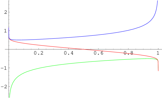
Figure 1: This shows the three functions, $w_{j}$, as a function of $x=\sin^{2}{\textstyle{\theta\over 2}}\displaystyle$ when $u$ is given by (4.82). One has $w_{1}<0$ and $w_{3}>0$ and $w_{2}$ has a simple zero at $\theta=\pi/2$. All three functions diverge at both ends of the interval.

We note that the forms given by (4.70) and (4.74) are still “harmonic” in that they are self-dual and closed. Moreover, $\Omega_{1}$ and $\Omega_{3}$ are non-singular in the wormhole geometry, except that $\Omega_{1}$ remains finite as $\theta\to 0$ while $\Omega_{3}$ remains finite as $\theta\to\pi$. This means that neither is square-integrable on the complete geometry. On the other hand, $\Omega_{2}$ falls off exponentially at both $\theta=0$ and $\theta=\pi$ but is singular at $\theta=\pi/2$, where the metric changes sign. Once again this last flux has a behavior precisely analogous to the two-form fields that were essential building blocks for the regular five-dimensional solutions that can be built from ambi-polar GH metrics.

Finally, we should comment that more general choices of $u(\theta)$, such as taking $c_{1}=-c_{2}=1$ in (4.58), can result in solutions with zeroes for $w_{1}$, $w_{2}$ and $w_{3}$. We have not studied these in detail.

5 The BPS solutions

5.1 Solving the BPS equations

Since there is only one independent harmonic form in the Atiyah-Hitchin metric, this means that the two-forms, $\Theta^{(I)}$, in (3.9) must all be proportional to one another for $I=1,2,3$. For simplicity, we will, in fact, take them all to be equal. We will also take the three warp factor functions to be equal, $Z_{I}=Z$, $I=1,2,3$. Ignoring, for the present, issues of regularity, the $SO(3)$ invariant solutions of (3.9) are given by the $\Omega_{i}$ of (4.70) and so we will take

$$\Theta^{(I)}~{}=~{}\Theta~{}=~{}\Omega_{1}~{}+~{}\Omega_{2}~{}+~{}\Omega_{3}\,.$$ (5.84)

The functions, $h_{j}$, in (4.74) contain integration constants, $\alpha_{j}$, that make this an arbitrary linear combination. Note: One should not confuse the index, $I=1,2,3$ on $\Theta^{(I)}$ with the index, $i=1,2,3$ on $\Omega_{i}$. The former indexes the $U(1)$ gauge groups of three-charge system while the latter labels the three distinct type of two-form in (4.70) that satisfy (3.9).

With this choice, the second BPS equation becomes:

$${d^{2}Z\over d\eta^{2}}~{}=~{}8\,\sum_{j=1}^{3}\,h_{j}^{2}\,a_{j}^{2}\,.$$ (5.85)

Given the form of $\Theta$, there is a unique Ansatz for the angular momentum vector, $k$:

$$k~{}=~{}\sum_{j=1}^{3}\,\mu_{j}\,\sigma_{j}\,,$$ (5.86)

which means that the third BPS equation yields three equations:

$${d\mu_{j}\over d\eta}\,~{}-~{}a_{j}^{2}\,\mu_{j}~{}=~{}3\,h_{j}\,a_{j}^{2}\,Z\,,\qquad{j=1,2,3}\,.$$ (5.87)

The factor of three comes from the sum over the $U(1)$ label, $I$, in (3.11) and the choices: $\Theta^{(I)}=\Theta$, $Z_{I}=Z$.

These equations can, once again, be integrated explicitly in terms of the the elliptic function, $u$. First, from (4.71) we have:

$${dZ\over d\eta}~{}=~{}\gamma_{0}~{}-~{}4\,\sum_{j=1}^{3}\,h_{j}^{2}\,,$$ (5.88)

for some constant, $\gamma_{0}$. Using (4.56) and (4.57) one can easily show that

$${d\over d\eta}\,{\alpha_{j}^{2}\over w_{j}}~{}=~{}u^{2}\,{d\over d\theta}\,{\alpha_{j}^{2}\over w_{j}}~{}=~{}\alpha_{j}^{2}~{}+~{}4\,(-1)^{j}\,h_{j}^{2}\,,$$ (5.89)

and hence:

$$Z~{}=~{}\delta~{}+~{}\gamma\,\eta~{}-~{}\sum_{j=1}^{3}\,(-1)^{j}\,{\alpha_{j}^{2}\over w_{j}}\,,$$ (5.90)

where $\gamma=\gamma_{0}+\sum_{j=1}^{3}(-1)^{j}\alpha_{j}^{2}$.

The last BPS equation, (5.87), can be integrated to yield:

$$\mu_{j}~{}=~{}{3\over h_{j}}\,\int h_{j}^{2}\,a_{j}^{2}\,Z\,d\eta~{}=~{}{3\over h_{j}}\,\int\Big{(}-{1\over 2}\,{d\over d\eta}h_{j}^{2}\Big{)}\,Z\,d\eta\,,\qquad{j=1,2,3}\,.$$ (5.91)

It is easy to integrate this explicitly. First, by integrating by parts one can show:

$${3\over h_{j}}\,\int h_{j}^{2}\,a_{j}^{2}\,\big{(}\delta~{}+~{}\gamma\,\eta)\,d\eta~{}=~{}-{\textstyle{3\over 2}}\displaystyle\,\delta\,h_{j}~{}-~{}{\textstyle{3\over 2}}\displaystyle\,\gamma\,\Big{[}\,h_{j}\eta~{}-~{}(-1)^{j}\,{\alpha_{j}^{2}\over 4\,h_{j}}\,\Big{(}{1\over w_{j}}-\eta\Big{)}\Big{]}~{}+~{}{\beta_{j}\over h_{j}}\,,$$ (5.92)

where the $\beta_{j}$ are constants of integration. The other parts of the integrals for $\mu_{j}$ can be obtained from:

$${3\over h_{j}}\,\int\,{h_{j}^{2}\,a_{j}^{2}\over w_{j}}\,d\eta = (-1)^{j}\,{\alpha_{j}^{2}\over 8\,h_{j}}\,\Big{[}\,{2\,w_{i}\,w_{k}\over w_{j}^{3}}~{}-~{}{w_{i}+w_{k}\over w_{j}^{2}}\,\Big{]}\,,$$

$${3\over h_{j}}\,\int\,{h_{j}^{2}\,a_{j}^{2}\over w_{i}}\,d\eta = (-1)^{j+1}\,{3\,\alpha_{j}^{2}\over 8\,h_{j}}\,{(w_{j}-w_{k})\over w_{j}^{2}}\,,$$ (5.93)

where $i,j,k\in\{1,2,3\}$ are all distinct.

Thus, rather surprisingly, we can obtain the complete solution analytically in terms of elliptic functions.

5.2 The bubbled solution on the standard Atiyah-Hitchin base

The physical intuition underlying BPS solutions is that all charges have to be of the same sign so that the electromagnetic repulsion balances the gravitational attraction. Bubbled geometries generically have geometric charges of all signs and then the attractive forces are balanced by threading cycles with fluxes that then resist the collapse of the bubbles. The result is then a stable configuration where the sizes of some of the bubbles are fixed in terms of the fluxes that thread them. Such relationships are typically embodied in a system of “Bubble Equations” [1, 11]. If one insists that a solution is a BPS configuration but one does not have the forces properly balanced then the solution is then supported only through the appearance of CTC’s. Thus, when investigating BPS geometries one typically encounters the constraints of bubble equations through the process of eliminating CTC’s.

The standard Atiyah-Hitchin base metric is, in its own right, a well-behaved BPS solution with no additional fluxes. Indeed, the addition of a flux through the non-trivial two-cycle should drive the configuration out of equilibrium and expand the bubble. We should therefore find irremovable CTC’s if we attempt to include a non-trivial flux. We now show that this is precisely what happens.

As we remarked earlier, the only non-trivial, harmonic flux on the standard Atiyah-Hitchin base is given by $\Omega_{1}$ and so we set $\alpha_{2}=\alpha_{3}=0$ in the results of the previous sub-section. We then find:

$$Z~{}=~{}\delta~{}+~{}\gamma\,\eta~{}+~{}{\alpha_{1}^{2}\over w_{1}}$$ (5.94)

and $k=\mu\sigma_{1}$, where

$$\mu = -{\textstyle{3\over 2}}\displaystyle\,\delta\,h_{1}~{}-~{}{\textstyle{3\over 2}}\displaystyle\,\gamma\,\Big{[}\,h_{1}\eta~{}+~{}\,{\alpha_{1}^{2}\over 4\,h_{1}}\,\Big{(}{1\over w_{1}}-\eta\Big{)}\Big{]}$$ (5.95)

$$~{}-~{}\,{\alpha_{1}^{4}\over 8\,h_{1}}\,\Big{[}\,{2\,w_{2}\,w_{3}\over w_{1}^{3}}~{}-~{}{w_{2}+w_{3}\over w_{1}^{2}}\,\Big{]}~{}+~{}{\beta_{1}\over h_{1}}\,.$$

It is interesting to note that the part of $Z$ corresponding to the flux sources in (5.94) (i.e. the $w_{1}^{-1}$ term) is always negative, and therefore at infinity this warp factor looks like it is coming from an object of negative mass and charge. This is however not surprising, considering that the Atiyah-Hitchin space also looks asymptotically as a negative-mass Taub-NUT space.

The value of $\beta_{1}$ is fixed by requiring that $\mu$ does not diverge, and indeed falls off at infinity. We find that if we set:

$$\beta_{1}~{}=~{}\frac{\pi^{2}\,\alpha_{1}^{4}}{8}\,,$$ (5.96)

then this removes all the terms that diverge at infinity and leaves only terms that fall off. Indeed, there are two types of such terms: Those proportional to $\gamma$, which fall off as ${1\over r}$, and the remainder that fall off as $re^{-r}$.

Near $\theta=0$ the function $\eta$ is logarithmically divergent and so $Z$ is logarithmically divergent unless $\gamma=0$. Physically, a non-zero value of $\gamma$ corresponds to a uniform distribution of M2 branes smeared over the bolt at $\theta=0$, with negative values of $\gamma$ corresponding to positive charge densities. If $\gamma=0$ then $Z=\delta-4\alpha_{1}^{2}$ at $\theta=0$.

For constant time slices, the five-dimensional metric (1.2) becomes

$$ds^{2}~{}=~{}\big{(}{\textstyle{1\over 4}}\displaystyle\,a^{2}\,Z~{}-~{}\mu^{2}\,Z^{-2}\big{)}\,\sigma_{1}^{2}~{}+~{}{\textstyle{1\over 4}}\displaystyle\,Z\,a^{2}\,b^{2}\,c^{2}\,d\eta^{2}~{}+~{}{\textstyle{1\over 4}}\displaystyle\,Z\,b^{2}\sigma_{2}^{2}~{}+~{}{\textstyle{1\over 4}}\displaystyle\,Z\,c^{2}\sigma_{3}^{2}\,,$$ (5.97)

and so to avoid CTC’s, one must have $Z\geq 0$ and the quantity:

$${\cal Q}~{}=~{}{\textstyle{1\over 4}}\displaystyle\,a^{2}\,Z^{3}~{}-~{}\mu^{2}\,$$ (5.98)

must be non-negative. The function $a(\theta)\sim\frac{1}{16}\theta^{2}$ as $\theta\to 0$ and $Z$ diverges, at worst, logarithmically. Thus we must have $\mu\to 0$ as $\theta\to 0$ in order to avoid CTC’s on the bolt. (This is how the bubble equations arise on GH spaces.) This means that we must take

$$\gamma~{}=~{}{\textstyle{1\over 4}}\displaystyle\,\delta~{}-~{}{\textstyle{2\over 3}}\displaystyle\,\alpha_{1}^{-2}\,\beta_{1}~{}=~{}{\textstyle{1\over 4}}\displaystyle\,\delta~{}-~{}{\textstyle{1\over 12}}\displaystyle\,\pi^{2}\,\alpha_{1}^{2}\,.$$ (5.99)

For pure-flux solutions, which have no singular sources, one must take $\gamma=0$ and the CTC condition (5.99) reduces to $\delta=\frac{1}{3}\,\pi^{2}\,\alpha_{1}^{2}$. Then one finds

$${\textstyle{1\over 4}}\displaystyle\,a^{2}\,Z~{}-~{}\mu^{2}\,Z^{-2}~{}\sim~{}-{\textstyle{1\over 3072}}\displaystyle\,(12-\pi^{2})\,\alpha_{1}^{2}\,\theta^{4}~{}<~{}0\,,$$ (5.100)

and so one necessarily has CTC’s in the immediate neighborhood of the bolt. This is a signal that there is no physical BPS solution based upon the standard Atiyah-Hitchin metric with pure flux: The flux will blow up the cycle and there is no gravitational attraction holding the bubble back.

One might hope that one could stabilize the solution with a distribution of M2 branes on the bolt. While this might be possible in general, it does not seem to be possible with a uniform, $SO(3)$ invariant distribution. For this, one must have $\gamma<0$ for $Z$ to remain positive near $\theta=0$ and then (5.99) means that $\alpha_{1}^{2}>{3\over\pi^{2}}\delta$. In addition, we must have $\delta\geq 0$ for $Z>0$ at infinity. From (5.88) one has

$${dZ\over d\eta}~{}=~{}\gamma~{}+~{}\alpha_{1}^{2}~{}-~{}4\,h_{1}^{2}~{}=~{}{\textstyle{1\over 4}}\displaystyle\,\delta~{}+~{}(1-{\textstyle{1\over 12}}\displaystyle\,\pi^{2})\,\alpha_{1}^{2}~{}-~{}4\,h_{1}^{2}\,,$$ (5.101)

and since $h_{1}=-\frac{1}{2}\,\alpha_{1}$ at $\theta=0$ and $h_{1}\to 0$ at infinity ($\theta=\pi$) we see that ${dZ\over d\eta}$ is negative at $\theta=0$ and positive at $\theta=\pi$. Therefore, $Z$ has a minimum for $\theta\in(0,\pi)$. While we have not done an exhaustive analysis, we generally find that $Z$ is negative at this minimum value. Some examples are shown in Fig. 2. Obviously, the complete five-dimensional metric is singular when $Z<0$.

Adding the singular M2-brane sources does render ${\cal Q}$ positive in a region around the bolt but, as one can see from (5.98), ${\cal Q}$ also goes negative shortly before $Z$ goes negative. Thus adding M2 branes sources moves CTC’s away from the bolt but at the cost of more extensive singular behavior elsewhere in the solution.

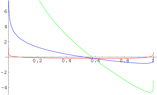
Figure 2: This shows plots of $Z$ as a function of $x=\sin^{2}{\textstyle{\theta\over 2}}\displaystyle$. We have taken $\delta=1$, fixed $\gamma$ in terms of $\alpha_{1}$ using (5.99) and then we have chosen three values of $\alpha_{1}$ that ensure that $\gamma$ is negative: $\alpha_{1}=0.6$, $\alpha_{1}=1.0$ and $\alpha_{1}=2.0$. The steeper graphs at $x=0.5$ correspond to larger values of $\alpha_{1}$. Note that $Z\to 1$ as $x\to 1$, but that $Z$ is generically negative for $x>0.6$.

5.3 Bubbling the ambi-polar Atiyah-Hitchin base

We now consider adding flux to one of the ambi-polar Atiyah-Hitchin metrics discussed in Section 4.3. That is, we will start with the ambi-polar “wormhole” geometry that arises from the choice (4.82), which therefore has the reflection symmetry given by (4.83). The solutions to the BPS equations have exactly the same functional form as those given in Section 5.1 for the standard Atiyah-Hitchin background. However, the underlying functions now have very different asymptotic behavior and this affects all of the choices based upon regularity and square integrability.

Let $r=-\log(\pi-\theta)$ and $\hat{r}=-\log(\theta)$, then as $\theta\to 0$ one has

$$u(\theta) \sim {\textstyle{1\over\pi}}\displaystyle\,\hat{r}\,e^{-{\hat{r}/2}}\,,\qquad\eta~{}\sim~{}-\eta_{0}~{}+~{}\frac{\pi^{2}}{\hat{r}}\,,$$

$$w_{1}(\theta) \sim -{\textstyle{1\over\pi^{2}}}\displaystyle\,\hat{r}^{2}\,,\quad w_{2}(\theta)~{}\sim~{}{\textstyle{1\over\pi^{2}}}\displaystyle\,\hat{r}\,,\quad w_{3}(\theta)~{}\sim~{}{\textstyle{1\over\pi^{2}}}\displaystyle\,\hat{r}\,,$$ (5.102)

which implies

$$a^{2}(\theta)~{}\sim~{}-{\textstyle{1\over\pi^{2}}}\displaystyle\,,\qquad b^{2}(\theta)~{}\sim~{}-{\textstyle{1\over\pi^{2}}}\displaystyle\,\hat{r}^{2}\,,\qquad c^{2}(\theta)~{}\sim~{}-{\textstyle{1\over\pi^{2}}}\displaystyle\,\hat{r}^{2}\,.$$ (5.103)

The constant, $\eta_{0}$, is defined by:

$$\eta_{0}~{}\equiv~{}\int_{0}^{\pi}\,{1\over u(\theta)^{2}}~{}=~{}2\pi\,.$$ (5.104)

As $\theta\to\pi$ one has:

$$u(\theta) \sim {\textstyle{1\over\pi}}\displaystyle\,r\,e^{-{r/2}}\,,\qquad\eta~{}\sim~{}-\frac{\pi^{2}}{r}\,,$$

$$w_{1}(\theta) \sim -{\textstyle{1\over\pi^{2}}}\displaystyle\,r\,,\quad w_{2}(\theta)~{}\sim~{}-{\textstyle{1\over\pi^{2}}}\displaystyle\,r\,,\quad w_{3}(\theta)~{}\sim~{}{\textstyle{1\over\pi^{2}}}\displaystyle\,r^{2}\,,$$ (5.105)

which implies

$$a^{2}(\theta)~{}\sim~{}{\textstyle{1\over\pi^{2}}}\displaystyle\,r^{2}\,,\qquad b^{2}(\theta)~{}\sim~{}{\textstyle{1\over\pi^{2}}}\displaystyle\,r^{2}\,,\qquad c^{2}(\theta)~{}\sim~{}{\textstyle{1\over\pi}}\displaystyle\,.$$ (5.106)

The metric in each of these asymptotic regions becomes:

$$ds^{2} \sim -{\textstyle{1\over 4\,\pi^{2}}}\displaystyle\,\big{(}d\hat{r}^{2}~{}+~{}\hat{r}^{2}(\sigma_{2}^{2}~{}+~{}\sigma_{3}^{2})~{}+~{}\sigma_{1}^{2}\big{)}\,,\qquad\theta\to 0\,,$$

$$ds^{2} \sim {\textstyle{1\over 4\,\pi^{2}}}\displaystyle\,\big{(}dr^{2}~{}+~{}r^{2}(\sigma_{1}^{2}~{}+~{}\sigma_{2}^{2})~{}+~{}\sigma_{3}^{2}\big{)}\,,\qquad\theta\to\pi\,.$$ (5.107)

We thus have an ambi-polar metric with two regions that are asymptotic to different $U(1)$ fibrations over different $\mathbb{R}^{3}$ bases. The metric changes sign precisely at $\theta=\frac{\pi}{2}$ at which point the metric function $b^{2}(\theta)$ has a simple pole, while $a^{2}(\theta)$ and $c^{2}(\theta)$ have simple zeroes.

This time the appropriate “harmonic” form is $\Omega_{2}$ because we have :

$$h_{1}(\theta) \sim -{\textstyle{1\over 2}}\displaystyle\,\alpha_{1}\,,\quad h_{2}(\theta)~{}\sim~{}{\textstyle{1\over 4}}\displaystyle\,\alpha_{2}\,\hat{r}\,e^{-{\hat{r}}}\,,\quad h_{3}(\theta)~{}\sim~{}{\textstyle{1\over 4}}\displaystyle\,\alpha_{3}\,\hat{r}\,e^{-{\hat{r}}}\,,\qquad\theta\to 0\,;$$

$$h_{1}(\theta) \sim -{\textstyle{1\over 4}}\displaystyle\,\alpha_{1}\,r\,e^{-{r}}\,,\quad h_{2}(\theta)~{}\sim~{}-{\textstyle{1\over 4}}\displaystyle\,\alpha_{2}\,r\,e^{-{r}}\,,\quad h_{3}(\theta)~{}\sim~{}{\textstyle{1\over 2}}\displaystyle\,\alpha_{3}\,,\qquad\theta\to\pi\,;$$ (5.108)

and so $\Omega_{2}$ is the only solution that falls off in both asymptotic regions. It is, however, not really harmonic in that it is singular precisely on the critical surface where $w_{2}=0$. This is, however, the standard behavior for the flux that goes into making the complete, five-dimensional solution and, as was noted in (3.41), the complete flux, $C^{(3)}$, is smooth on the critical surface.

One now has

$$Z~{}=~{}\delta~{}+~{}\gamma\,\eta~{}-~{}{\alpha_{2}^{2}\over w_{2}}$$ (5.109)

and $k=\mu\sigma_{2}$, where

$$\mu = -{\textstyle{3\over 2}}\displaystyle\,\delta\,h_{2}~{}-~{}{\textstyle{3\over 2}}\displaystyle\,\gamma\,\Big{[}\,h_{2}\eta~{}-~{}\,{\alpha_{2}^{2}\over 4\,h_{2}}\,\Big{(}{1\over w_{2}}-\eta\Big{)}\Big{]}$$ (5.110)

$$~{}-~{}\,{\alpha_{2}^{4}\over 8\,h_{2}}\,\Big{[}\,{2\,w_{1}\,w_{3}\over w_{2}^{3}}~{}-~{}{w_{1}+w_{3}\over w_{2}^{2}}\,\Big{]}~{}+~{}{\beta_{2}\over h_{2}}\,.$$

Recall that the vector potential for $\Omega_{2}$ is given in (4.73) and so the potential for the complete Maxwell field is:

$$A~{}=~{}Z^{-1}\,\big{(}dt+\mu\,\sigma_{2}\big{)}~{}-~{}h_{2}\,\sigma_{2}\,.$$ (5.111)

and so the only potentially singular term is:

$$Z^{-1}\,\mu~{}-~{}h_{2}~{}\sim~{}-{\alpha_{2}\over 4\,u^{2}\,w_{2}}\,(4\,w_{1}\,w_{3}~{}+~{}u^{4})\,,$$ (5.112)

as $w_{2}\to 0$. However, from (4.57) one has

$$w_{1}\,w_{3}~{}+~{}{\textstyle{1\over 4}}\displaystyle\,u^{4}~{}=~{}w_{2}\,(w_{1}+w_{3})-w_{2}^{2}\,,$$ (5.113)

and so the complete Maxwell field is regular.

The spatial sections of the complete five-dimensional metric are:

$$ds^{2}~{}=~{}\big{(}{\textstyle{1\over 4}}\displaystyle\,b^{2}\,Z~{}-~{}\mu^{2}\,Z^{-2}\big{)}\,\sigma_{2}^{2}~{}+~{}{\textstyle{1\over 4}}\displaystyle\,Z\,a^{2}\,b^{2}\,c^{2}\,d\eta^{2}~{}+~{}{\textstyle{1\over 4}}\displaystyle\,Z\,a^{2}\sigma_{1}^{2}~{}+~{}{\textstyle{1\over 4}}\displaystyle\,Z\,c^{2}\sigma_{3}^{2}\,.$$ (5.114)

First note that:

$$Z\,a^{2} = {w_{3}\over w_{1}}\,((\delta~{}+~{}\gamma\,\eta)\,w_{2}~{}-~{}\alpha_{2}^{2})\,,\qquad Z\,c^{2}~{}=~{}{w_{1}\over w_{3}}\,((\delta~{}+~{}\gamma\,\eta)\,w_{2}~{}-~{}\alpha_{2}^{2})\,,$$

$$Z\,a^{2}\,b^{2}\,c^{2} = \,w_{1}\,w_{3}((\delta~{}+~{}\gamma\,\eta)\,w_{2}~{}-~{}\alpha_{2}^{2})\,.$$ (5.115)

Since one has $w_{1}<0$ and $w_{3}>0$ everywhere (see Fig.1) it follows that these three metric coefficients are regular and positive near $w_{2}=0$.

More generally, observe that $\delta+\gamma\eta\to\delta$ and $w_{2}\to-\infty$ as $\theta\to\pi$ and $\delta+\gamma\eta\to\delta-2\pi\gamma$ and $w_{2}\to+\infty$ as $\theta\to 0$. This means that for the metric coefficients in (5.115) to remain positive at infinity one must have:

$$\gamma~{}\geq~{}{\delta\over 2\pi}~{}\geq~{}0\,.$$ (5.116)

Indeed observe that the function, $\eta+{\textstyle{1\over 2}}\displaystyle\eta_{0}$, is odd under $\theta\to\pi-\theta$ and so, for $\gamma>0$, the function

$$\gamma(\eta+{\textstyle{1\over 2}}\displaystyle\eta_{0})\,w_{2}~{}=~{}\gamma(\eta+\pi)\,w_{2}$$ (5.117)

is globally negative with a double zero at $\theta={\pi\over 2}$. Thus the metric coefficients (5.115) are globally positive when $\delta$ is the middle of the range specified by (5.116).

Now consider the remaining coefficient, $Z^{-2}{\cal Q}$, where

$${\cal Q}~{}\equiv~{}{\textstyle{1\over 4}}\displaystyle\,b^{2}\,Z^{3}~{}-~{}\mu^{2}\,.$$ (5.118)

Near $w_{2}=0$ one has $Z^{-2}\sim\alpha_{2}^{-4}w_{2}^{2}$ and

$${\cal Q}~{}\sim~{}{\alpha_{2}^{6}\,w_{1}\,w_{3}\over u^{4}\,w_{2}^{4}}\,\big{(}w_{2}\,(w_{1}+w_{3})~{}-~{}(w_{1}\,w_{3}+{\textstyle{1\over 4}}\displaystyle\,u^{4})\big{)}~{}+~{}{\cal O}(w_{2}^{-2})\,.$$ (5.119)

However, it follows from (5.113) that, in fact, ${\cal Q}\sim{\cal O}(w_{2}^{-2})$ and so the metric coefficient $Z^{-2}{\cal Q}$ is regular around $w_{2}=0$.

The regularity of the solution near the critical surface was, of course, guaranteed by our general analysis of the Toda metrics in Section 3, but it is still useful to see how it comes about here.

Finally there is the angular momentum vector and the issue of global positivity of ${\cal Q}$. For this it is most convenient to consider the combination $h_{2}\,\mu$:

$$h_{2}\,\mu \sim {\textstyle{3\over 8}}\displaystyle\,\gamma\,\eta_{0}\,\alpha_{2}^{2}~{}+~{}\beta_{2}~{}+~{}{\textstyle{1\over 8}}\displaystyle\,\pi^{2}\,\alpha_{2}^{4}~{}+~{}{\cal O}(\theta^{2})\,,\qquad\theta\to 0\,,$$ (5.120)

$$h_{2}\,\mu \sim \beta_{2}~{}-~{}{\textstyle{1\over 8}}\displaystyle\,\pi^{2}\,\alpha_{2}^{4}~{}+~{}{\cal O}((\pi-\theta)^{2})\,,\qquad\theta\to\pi\,.$$ (5.121)

Since $h_{2}$ vanishes exponentially fast in $r$ and $\hat{r}$ in the two asymptotic regions (see (5.108)), this means that $\mu$ will diverge exponentially in $r$ and $\hat{r}$ unless

$$\beta_{2}~{}=~{}{\textstyle{1\over 8}}\displaystyle\,\pi^{2}\,\alpha_{2}^{4}\,,\qquad\gamma~{}=~{}-{\textstyle{2\over 3}}\displaystyle\,\pi^{2}\,\eta_{0}^{-1}\,\alpha_{2}^{2}~{}=~{}-{\textstyle{1\over 3}}\displaystyle\,\pi\,\alpha_{2}^{2}\,.$$ (5.122)

If these two conditions are met then $\mu$ also vanishes exponentially in $r$ and $\hat{r}$ in both of the asymptotic regions.

Unfortunately this value of $\gamma$ is inconsistent with (5.116). If one allows $\mu$ to diverge exponentially in one of the asymptotic regions then ${\cal Q}$ will become negative in the asymptotic regions. This is because $Z$ limits to a finite value and $b^{2}$ diverges as a power of $r$ or $\hat{r}$. Therefore there is no way to arrange the metric to be positive definite in the asymptotic regions on both sides of the wormhole: Either one has (5.116) and arranges that three coefficients in (5.115) to be globally positive, or one arranges that ${\cal Q}>0$ only to have the three coefficients in (5.115) to change sign in one of the asymptotic regions.

Thus we have a beautifully regular metric across the critical surface, but it fails to be globally well-behaved as a “wormhole” metric. We suspect that the problem is due to the high level of symmetry. With more bubbles and thus more parameters we believe that one could simultaneously control behavior in both asymptotic regions. Even with the very high level of symmetry, there is another way to remove the regions of CTC’s.

5.4 Pinching off the wormhole

One way to remove the region of CTC’s is to pinch off the wormhole before one encounters the region where CTC’s occur. Here we will consider the ambi-polar metric described exactly as above with the asymptotic regions as $\theta\to\pi$ arranged to be regular and asymptotic to the $U(1)$ fibration over $\mathbb{R}^{3}$ as in (5.107). This requires one to take:

$$\beta_{2}~{}=~{}{\textstyle{1\over 8}}\displaystyle\,\pi^{2}\,\alpha_{2}^{4}\,,\qquad\delta~{}>~{}0\,.$$ (5.123)

The metric coefficients, $a_{i}^{2}$, are non-vanishing away from the critical surface, and so to pinch off the complete metric away from the critical surface we must arrange that the function $Z$ vanish at some point. To avoid CTC’s one must also ensure that ${\cal Q}$ is non-negative near the pinch-off and so one must arrange that $\mu$ vanishes simultaneously with $Z$. Thus we are looking for a point, $\theta_{0}$, such that

$$Z\big{|}_{\theta=\theta_{0}}~{}=~{}0\,,\qquad\mu|_{\theta=\theta_{0}}~{}=~{}0\,.$$ (5.124)

Given these conditions, the equation of motion, (5.87), for $\mu$ then implies that $\frac{d}{d\theta}\mu$ must also vanish at $\theta_{0}$. Therefore, near the pinching-off point we have:

$$Z~{}\sim~{}z_{0}\,(\theta-\theta_{0})\,,\qquad\mu~{}\sim~{}\mu_{0}\,(\theta-\theta_{0})^{2}\,,\qquad\big{(}{\textstyle{1\over 4}}\displaystyle\,b^{2}\,Z~{}-~{}\mu^{2}\,Z^{-2}\big{)}~{}\sim~{}{\textstyle{1\over 4}}\displaystyle\,b_{0}^{2}\,z_{0}(\theta-\theta_{0})\,.$$ (5.125)

This means that the spatial part of the complete metric (5.114) is indeed pinching off in every direction with surfaces of constant $\theta$ being a set of collapsing, squashed three-spheres. The metric is not smooth at $\theta_{0}$: There is a curvature singularity in the spatial part of the metric and the coefficient of $dt^{2}$ is diverging as $(\theta-\theta_{0})^{-2}$. This reflects a similar divergence in the electric component of the Maxwell fields, $A^{(I)}$, (see (3.8)) at $Z=0$. One should also note that the flux, $\Theta$, is also singular at $Z=0$ in that it remains constant while the cycle that supports it is collapsing.

Define

$$\hat{\gamma}~{}\equiv~{}\alpha_{2}^{-2}\,\gamma\,,\qquad\hat{\delta}~{}\equiv~{}\alpha_{2}^{-2}\delta\,,$$ (5.126)

then the conditions (5.124) relate $\hat{\gamma}$ and $\hat{\delta}$ to $\theta_{0}$. Thus we can, in principle, choose the pinching-off point and then (5.124) yields the corresponding values of $\hat{\gamma}$ and $\hat{\delta}$. In practice, there is the constraint that $\delta>0$. We know from the analysis above that we cannot arrange for $Z$ and $\mu$ to vanish simultaneously at $\theta=0$. Numerical analysis shows that one cannot have $Z$ and $\mu$ vanish simultaneously unless $\theta_{0}\gtrsim 0.6158$. Since we are interested in solutions that contain the critical surface ($w_{2}=0$), we have found a number of solutions that pinch off for $0.6158\lesssim\theta_{0}<\frac{\pi}{2}$. We also checked numerically that it does not appear to be possible to have all three of $\mu$, $Z$ and ${dZ\over d\theta}$ vanish simultaneously for $\theta\in(0,\frac{\pi}{2})$. Thus (5.125) appears to be the general behavior at a pinch-off: $Z$ does not appear to be able to have a double root.

         

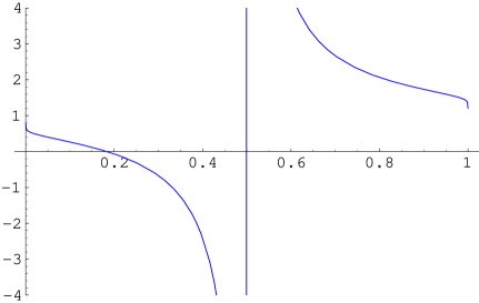
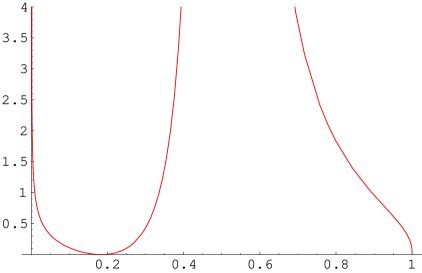
Figure 3: These are graphs of $Z$ (on the left) and $\mu$ (on the right) as functions of $x=\sin^{2}{\textstyle{\theta\over 2}}\displaystyle$ for $\gamma=0$, $\delta=1$ and $\alpha_{2}\approx 0.4890$. Both functions are singular at $x=0.5$ and both vanish, $\mu$ with a double root, at $x\approx 0.1837$.

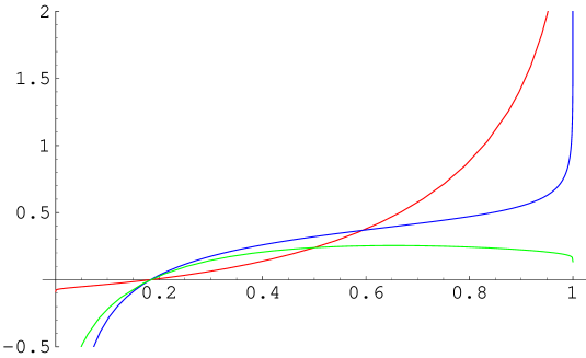
Figure 4: This graph shows the three metric coefficients in the angular directions, $Za^{2}$, $Z^{-2}{\cal Q}$ and $Zc^{2}$ (in this order from top to bottom on the right-hand side of the graph), as functions of $x=\sin^{2}{\textstyle{\theta\over 2}}\displaystyle$ for $\gamma=0$, $\delta=1$ and $\alpha_{2}\approx 0.4890$. All of these functions vanish at the pinching-off point, $x\approx 0.1837$, and are positive-definite to the right of it.

We have verified in several numerical examples that the spatial metric is indeed globally positive definite in the region at and to the right of the pinch. These solutions still contain the critical surface where the $a_{i}^{2}$ and $Z$ simultaneously change sign and these solutions are perfectly regular across the critical surface. The cost of ensuring the global absence of CTC’s is to include a non-standard, singular point-source at the center of the solution.

To present an example, we considered the solution with $\gamma=0$, $\delta=1$. Solving (5.124) leads to $\alpha_{2}\approx 0.4890$ and the pinch-off at $x=\sin^{2}(\frac{\theta}{2})\approx 0.1837$. In Fig. 3 we show plots of the functions $Z$ and $\mu$ for these parameter values. Note that both are singular at $x=0.5$ and that both vanish, $\mu$ with a double root, at $x\approx 0.1837$. In Fig. 4 we have shown the three metric coefficients in the angular directions, $Za^{2}$, $Zc^{2}$ and $Z^{-2}{\cal Q}$. All of them are positive and vanish exactly at the pinching-off point.

Before ending this section we should make a few more comments about the metric that is pinching off. The singularity at the pinch-off point is caused by the fact that the warp factors $Z_{I}$ go to zero. This causes the size of the two-cycles wrapped by fluxes to shrink to zero size, and hence the energy density coming from these fluxes to be infinite. A well-known solution with a similar type of singularity is the one obtained by Klebanov and Tseytlin [31]. However, for this solution it is well understood that the singularity comes about because of the high level of symmetry in the Ansatz, and that upon considering a less-symmetric base space the singularity is resolved [32]. Since the base space considered here also has a high level of symmetry, it is tempting to conjecture that, in analogy to the Klebanov-Strassler solution [32], the pinching off will be resolved by the blowing up of a two-cycle on the base, which will only be possible in a less-symmetric, non-singular background.

We should also remark that in our discussion we have taken all three warp factors to be equal, but generically we can also imagine pinching off the metric using only one of the warp factors, and keeping the others finite. This will change the structure of the metric near the singularity (some of the two-tori will blow up and some others will shrink), but the singularity will also come from shrinking cycles on the base, and will probably be resolved also by considering a less-symmetric base with a blown-up two-cycle

6 Variations on the Eguchi-Hanson metric

Given the foregoing results, particularly those involving wormholes, it is interesting to look at the corresponding story for the Eguchi-Hanson metric [35]. This metric has an $SO(3)\times U(1)$ invariance and the diagonal $U(1)$ action is triholomorphic. The metric is equivalent to a GH metric with two GH points of equal charge [36]. The manifestly $SO(3)\times U(1)$ invariant form of this metric is:

$$ds^{2}=\bigg{(}1-\frac{a^{4}}{\rho^{4}}\bigg{)}^{-1}\,d\rho^{2}~{}+~{}\frac{\rho^{2}}{4}\bigg{(}1-\frac{a^{4}}{\rho^{4}}\bigg{)}\sigma_{3}^{2}~{}+~{}\frac{\rho^{2}}{4}(\sigma_{1}^{2}+\sigma_{2}^{2})\,.$$ (6.127)

The space contains an $S^{2}$ (bolt) at $\rho=a$ and so the range of the radial coordinate is $a\leq\rho<\infty$. At infinity this space is asymptotic to $\mathbb{R}^{4}/\mathbb{Z}_{2}$.

To avoid closing off of the space at the bolt, we analytically continue by taking $a^{2}=ib$, with $b$ real, and introduce a new radial coordinate $\eta=\rho^{2}$. One thereby obtains:

$$ds^{2}=\bigg{(}1+\frac{b^{2}}{\eta^{2}}\bigg{)}^{-1}\frac{d\eta^{2}}{4\eta}+~{}\frac{\eta}{4}(\sigma_{1}^{2}+\sigma_{2}^{2})+~{}\frac{\eta}{4}\bigg{(}1+\frac{b^{2}}{\eta^{2}}\bigg{)}\sigma_{3}^{2}\,.$$ (6.128)

This metric was also considered by Eguchi and Hanson in [33], where it was called “type I,” and was given in the form:

$$ds^{2}=\left(1+\left(1-\displaystyle\frac{a^{4}}{r^{4}}\right)^{-1/2}\right)^{2}\displaystyle\frac{dr^{2}}{4}+\displaystyle\frac{r^{2}}{8}\left(1+\left(1-\displaystyle\frac{a^{4}}{r^{4}}\right)^{1/2}\right)(\sigma_{1}^{2}+\sigma_{2}^{2})+\displaystyle\frac{r^{2}}{4}\sigma_{3}^{2}\,.$$ (6.129)

This may be mapped to (6.128) via the coordinate change

$$\eta~{}=~{}r^{2}\left(1+\sqrt{1-\displaystyle\frac{a^{4}}{r^{4}}}\right)\,.$$ (6.130)

In terms of the Toda frame, (2.3)–(2.6), this metric was found in [28] and is given by

$$\nu=\log\left(z^{2}+\frac{a^{4}}{16}\right)-\log(2)-2\log\left(1+\frac{x^{2}+y^{2}}{8}\right)\,.$$ (6.131)

The reason why this metric was never studied in the past is that it is not geodesically complete, and there is a singularity at $\eta=0$. Nevertheless, we can extend the coordinate $\eta=\rho^{2}$ to negative values, and the resulting space (6.128) has two regions, one where the signature is $(+,+,+,+)$ and one where the signature is $(-,-,-,-)$ . This makes (6.128) into precisely an ambi-polar metric of the type that can give a good five-dimensional BPS solution: The overall sign of the metric changes as one passes through $\eta=0$, with the coefficient of a $U(1)$ fiber becoming singular at this critical surface.

6.1 The BPS solutions

In order to solve the BPS equations, (3.9)–(3.11), it is convenient to introduce the basis of frames given by:

$$\hat{e}_{1}=-\left(1+\frac{b^{2}}{\eta^{2}}\right)^{-1/2}\frac{d\eta}{2\sqrt{\eta}}\,,\qquad\hat{e}_{2}=\frac{\sqrt{\eta}}{2}\sigma_{1}\,,\qquad\hat{e}_{3}=\frac{\sqrt{\eta}}{2}\sigma_{2}\,,\qquad\hat{e}_{4}=\displaystyle\frac{\sqrt{\eta}}{2}\left(1+\frac{b^{2}}{\eta^{2}}\right)^{1/2}\sigma_{3}$$ (6.132)

One can then show that:

$$\Theta=\frac{\alpha}{\eta^{2}}(\hat{e}_{1}\wedge\hat{e}_{4}+\hat{e}_{2}\wedge\hat{e}_{3})$$ (6.133)

defines a harmonic, self-dual, “normalizable” two form for constant $\alpha$. One also has $\Theta=dB$ with $B=\displaystyle\frac{\alpha}{4\eta}\sigma_{3}$. As before, we take all three flux forms $\Theta^{(I)}$ to be equal to $\Theta$ and set $Z_{I}=Z$. Then the equation for $Z(\eta)$ becomes

$$\frac{d}{d\eta}\left((\eta^{2}+b^{2})\frac{dZ}{d\eta}\right)=\frac{\alpha^{2}}{2\eta^{3}}$$ (6.134)

which is solved by

$$Z(\eta)=\gamma+\frac{\alpha^{2}}{4b^{2}\eta}+\left(\frac{\alpha^{2}}{4b^{3}}+\frac{\beta}{b}\right)\arctan\left(\frac{\eta}{b}\right)\,,$$ (6.135)

where $\beta$ and $\gamma$ are integration constants. The angular momentum vector, $k$, has a solution of the form $k=\mu(\eta)\sigma_{3}$ where the function $\mu(\eta)$ satisfies

$$\eta^{3}\frac{d\mu}{d\eta}-\eta^{2}\mu+\frac{3\alpha\gamma}{4}\eta+\frac{3\alpha}{4}\left(\frac{\alpha^{2}}{4b^{3}}+\frac{\beta}{b}\right)\arctan\left(\frac{\eta}{b}\right)+\frac{3\alpha^{3}}{16b^{2}}=0\,.$$ (6.136)

The solution to this equation is

$$\mu(\eta)=\delta\eta+\frac{3\alpha}{8b^{2}}\left(\frac{\alpha^{2}}{4b^{2}}+\beta\right)+\frac{3\alpha\gamma}{8}\frac{1}{\eta}+\frac{\alpha^{3}}{16b^{2}}\frac{1}{\eta^{2}}+\frac{3\alpha}{8b^{3}}\left(\frac{\alpha^{2}}{4b^{2}}+\beta\right)\eta\arctan\left(\frac{\eta}{b}\right)+\\ \frac{3\alpha}{8b}\left(\frac{\alpha^{2}}{4b^{2}}+\beta\right)\frac{1}{\eta}\arctan\left(\frac{\eta}{b}\right)\,.$$ (6.137)

To complete the solution we have to impose boundary condition on the functions $Z$ and $\mu$.

6.2 A regular “wormhole”

If the solution is to have two asymptotic regions corresponding to $\eta\rightarrow\pm\infty$ then we must require that the angular momentum vector falls off in these regions or there will generically be CTC’s. This implies:

$$\delta=0\,,\qquad\qquad\beta=-\displaystyle\frac{\alpha^{2}}{4b^{2}}\,,$$ (6.138)

and then the functions $Z$ and $\mu$ simplify to:

$$Z(\eta)=\gamma+\frac{\alpha^{2}}{4b^{2}\eta}\,,\qquad\mu(\eta)=\frac{3\alpha\gamma}{8}\frac{1}{\eta}+\frac{\alpha^{3}}{16b^{2}}\frac{1}{\eta^{2}}\,.$$ (6.139)

If $\gamma\neq 0$, $Z$ will have a zero at $\eta=-\frac{\alpha^{2}}{4b^{2}\gamma}$ and thus we will inevitably have CTC’s unless we pinch off the solution before, or at, this point.

We consider $\gamma=0$ first, for which we have:

$$Z=\displaystyle\frac{\alpha^{2}}{4b^{2}}\frac{1}{\eta}\,,\qquad\qquad\mu=\displaystyle\frac{\alpha^{3}}{16b^{2}}\frac{1}{\eta^{2}}\,.$$ (6.140)

Note that the angular momentum function $\mu$ is always positive and is diverging on the critical surface $\eta=0$. The $Z$ also diverges and changes sign on the critical surface. This behavior ensures that the five-dimensional metric is regular and Lorentzian. The explicit form of the space-time metric is:

$$ds^{2}_{5}=-\displaystyle\frac{16b^{4}}{\alpha^{4}}\eta^{2}dt^{2}-\displaystyle\frac{2b^{2}}{\alpha}dt\,\sigma_{3}+\displaystyle\frac{\alpha^{2}}{16b^{2}}\displaystyle\frac{d\eta^{2}}{(\eta^{2}+b^{2})}+\displaystyle\frac{\alpha^{2}}{16b^{2}}(\sigma_{1}^{2}+\sigma_{2}^{2}+\sigma_{3}^{2})\,.$$ (6.141)

This metric can be cast into a more familiar form by first diagonalizing the metric by shifting the $\psi$-coordinate in (3.47) so that $\sigma_{3}\rightarrow\sigma_{3}+\displaystyle\frac{16b^{4}}{\alpha^{3}}dt$:

$$ds^{2}_{5}=-\displaystyle\frac{16b^{4}}{\alpha^{4}}(\eta^{2}+b^{2})dt^{2}+\displaystyle\frac{\alpha^{2}}{16b^{2}}\displaystyle\frac{d\eta^{2}}{\eta^{2}+b^{2}}+\displaystyle\frac{\alpha^{2}}{16b^{2}}(\sigma_{1}^{2}+\sigma_{2}^{2}+\sigma_{3}^{2})\,.$$ (6.142)

Change variables via $\eta=b\sinh\chi$, $\tilde{t}=\displaystyle\frac{16b^{4}}{\alpha^{3}}t$ and then the metric becomes

$$ds^{2}_{5}=\displaystyle\frac{\alpha^{2}}{16b^{2}}\,(-\cosh^{2}\chi\,d\tilde{t}^{2}+d\chi^{2}+\sigma_{1}^{2}+\sigma_{2}^{2}+\sigma_{3}^{2})\,,$$ (6.143)

which is the well known metric for global $AdS_{2}\times S^{3}$. The complete Maxwell field on this space is given by

$$dA~{}=~{}d\Theta-d(Z^{-1}(dt+k))\,,$$ (6.144)

and, using $\Theta=dB$ with $B=\displaystyle\frac{\alpha}{4\eta}\sigma_{3}$, we find

$$A~{}=~{}-\displaystyle\frac{4b^{2}}{\alpha^{2}}\,\eta\,dt\,,\qquad F~{}=~{}\displaystyle\frac{4b^{2}}{\alpha^{2}}\,dt\wedge d\eta\,.$$ (6.145)

The Maxwell field is thus proportional to the volume form on $AdS_{2}$ and we have obtained the global form of a Robinson-Bertotti solution. The wormhole thus reduces to the usual global AdS solution.

In fact the solution based on the singular EH metric (6.128) (with $\eta>0$) has also been discussed in [9], where it was shown to give an $AdS_{2}\times S^{3}$ solution with the $AdS_{2}$ in global coordinates. What we find very puzzling is the fact that in order to get the entire range of coordinates for the global $AdS_{2}$ metric, one must start from the ambi-polar EH metric with the coordinate $\eta$ running between $-\infty$ and $\infty$.

It is interesting to try to understand the reason for which we could find an Eguchi-Hanson “wormhole” but not an Atiyah-Hitchin one. At an algebraic level, the problem comes from the form of $\mu$, which in the Eguchi-Hanson background goes to zero on both asymptotic regions (6.139), while in the Atiyah-Hitchin background $\mu$, (5.95), diverges in one region or in the other. If one relaxes the requirement that the Atiyah-Hitchin solutions be asymptotically flat, one can choose a more generic $\Theta$, containing all three $\Omega_{i}$. However, this still does not give a $\mu$ that decays properly at the two asymptotic regions.

6.3 A “pinch-off” solution

The other way to remove CTC’s is to allow $\gamma\neq 0$ in (6.135) and pinch-off the asymptotic region with $\eta\to-\infty$ at the point, $\eta_{0}$, where $Z$ vanishes. This means that we only have to require that $\mu$ vanish as $\eta\rightarrow\infty$ and this implies

$$\delta=-\frac{3\pi\alpha}{16b^{3}}\left(\beta+\frac{\alpha^{2}}{4b^{2}}\right)$$ (6.146)

in (6.137).

As with the Atiyah-Hitchin solution, the solution will have CTC’s near the pinching off point unless we also require that $\mu$ vanishes at the same point. Specifically, the constant time slices of the metric have the form:

$$ds^{2}=-\frac{\mu^{2}}{Z^{2}}\,\sigma_{3}^{2}+Z\left(\left(1+\frac{b^{2}}{\eta^{2}}\right)^{-1}\frac{d\eta^{2}}{4\eta}+\frac{\eta}{4}(\sigma_{1}^{2}+\sigma_{2}^{2})+\frac{\eta}{4}\left(1+\frac{b^{2}}{\eta^{2}}\right)\sigma_{3}^{2}\right)$$ (6.147)

and to avoid CTC’s we must have

$${\cal Q}~{}\equiv~{}Z^{3}\left(\frac{\eta^{2}+b^{2}}{4\eta}\right)-\mu^{2}~{}\geq~{}0\,.$$ (6.148)

If $Z$ vanishes then $\mu$ must vanish and this imposes a relationship, akin to the bubble equations, on $\beta$, $\alpha$ and $b$. Unlike the corresponding solution in the Atiyah-Hitchin background, there is still a free parameter in the final result, and if one choses these parameters in the proper ranges one can arrange that the pinch-off occurs at $\eta_{0}<0$ and that there are no CTC’s in the region $\eta>\eta_{0}$. There is still, however, a curvature singularity in the metric at $\eta=\eta_{0}$, similar to the one in the pinched-off Atiyah-Hitchin solution, and probably caused also by the fact that the ansatz used is very symmetric. It is quite likely that this singularity will also be resolved in the same manner as the Klebanov-Tseylin/Klebanov-Strassler solutions [31, 32]

It is easy to find numerical examples that exhibit a “pinch off.” For example, one can take the following values of the parameters:

$$\alpha\approx 4.2619\qquad\beta\approx-4.5358\qquad\gamma=b=1\qquad\text{and}\qquad\delta=-\frac{3\pi\alpha}{16b^{3}}\left(\beta+\frac{\alpha^{2}}{4b^{2}}\right)\,,$$ (6.149)

and the pinch off point is $\eta_{0}\approx-4.5721$. Since $\eta_{0}$ is negative this represents a solution based upon a non-trivial ambi-polar base metric.

7 Conclusions

We have investigated the construction of three-charge solutions that do not have a tri-holomorphic $U(1)$ isometry. We have found that the most general form of these solutions, can be expressed in term of several scalar functions. One of these functions satisfies the (non-linear) $SU(\infty)$ Toda equation, while the other functions satisfy linear equations that can be thought of as various linearizations of the $SU(\infty)$ Toda equation.

We have also shown generically that in the region where the signature of the four-dimensional base space changes from $(+,+,+,+)$ to $(-,-,-,-,)$, the fluxes, warp factors, and the rotation vector diverge as well, but the overall five-dimensional (or eleven-dimensional) solution is smooth. This is similar to what happens when the base-space is Gibbons-Hawking, and strongly suggests that this phenomenon is generic: Any ambi-polar, four-dimensional, hyper-Kähler metric with at least one non-trivial two-cycle can be used to construct a regular supersymmetric five-dimensional three-charge solution upon adding fluxes, warp factors and rotation according to the BPS equations (3.9), (3.10) and (3.11).

This phenomenon is likely to be quite important in the programme of establishing whether black holes are ensembles of smooth supergravity or string solutions. To prove this conjecture, one would need to construct and count smooth horizonless solutions that have the same charges and angular momenta as three-charge black holes or black rings. Our analysis suggests that this counting problem is in fact much easier, since one would not have to count the full solutions, but just the hyper-Kähler base spaces underlying them. It also suggests that we may be able to capture the essential structure of the hyper-Kähler base by approximating it with a quilt of GH spaces.

Since the most general form of hyper-Kähler, four-dimensional spaces with a rotational $U(1)$ isometry is not known explicitly, one cannot explicitly construct the most general three-charge bubbling solution with this isometry. Nevertheless, we have been able to construct a first explicit bubbling solution with a rotational $U(1)$ starting from an ambi-polar generalization of the Atiyah-Hitchin metric. For both the standard Atiyah-Hitchin and Eguchi-Hanson metrics, it is not possible to construct regular three-charge bubbling solutions. This reflects the fact that fluxes tend to stabilize cycles that would shrink by themselves, and hence only “pathological” generalizations to ambi-polar metrics can be used as base-spaces to create bubbling solutions. We have obtained the ambi-polar generalizations of both the Atiyah-Hitchin and the Eguchi-Hanson spaces, and have constructed the full three-charge solutions based on these spaces.

As expected from our general analysis, the full solutions are completely regular at the critical surface where the metric on the base space changes sign. Moreover, for the ambi-polar Eguchi-Hanson space, one can construct the full solution, which, interestingly enough, turns out to be global $AdS_{2}\times S^{3}$. We could also obtain solutions that pinch off, and have a curvature singularity. We argued that this singularity has the same structure as the one in the Klebanov-Tseytlin solution [31] and we believe the presence of this singularity is a consequence of the high level of symmetry of the base space, and that the singularity will similarly be resolved by considering a less-symmetric base space.

This work opens several interesting directions of research. First, having shown that singular, $U(1)$-invariant, ambi-polar, four-dimensional, hyper-Kähler metrics can give smooth five-dimensional solutions upon adding fluxes, it is important to go back to the $SU(\infty)$ Toda equation and to construct more general solutions. A first step in this investigation would be to find the solutions of the Toda equations that give the $U(1)\times U(1)$ invariant ambi-polar Gibbons-Hawking metrics, following perhaps the techniques of [29]. One could then find other solutions in the vicinity of the latter, and count them using the techniques of [37].

Second, the fact that the ambi-polar generalizations of the Atiyah-Hitchin and the Eguchi-Hanson spaces give regular geometries suggests that ambi-polar generalizations of other known hyper-Kähler metrics will also give regular solutions. Finding these solutions would be quite interesting.

Finally, we have seen that the ambi-polar generalization of the Eguchi-Hanson space yields a full geometry that is $AdS_{2}\times S^{3}$. Moreover, unlike in the case of usual bubbling BPS solutions, the $AdS_{2}$ solution is not the Poincaré patch, but the full global $AdS$ solution. While the distinction between global and Poincaré $AdS_{2}$ is relatively trivial, the appearance of something like a regular wormhole suggests that bubbling geometries might be even richer and more interesting than was originally anticipated.

Acknowledgements

We would like to thank Juan Maldacena and Radu Roiban for interesting discussions. The work of NB and NW was supported in part by funds provided by the DOE under grant DE-FG03-84ER-40168. The work of IB was supported in part by the Diréction des Sciences de la Matière of the Commissariat à L’Enérgie Atomique of France. The work of NB was also supported in part by the Dean Joan M. Schaefer Research Scholarship.

References

- [1] I. Bena and N. P. Warner, “Bubbling supertubes and foaming black holes,” Phys. Rev. D 74, 066001 (2006) [arXiv:hep-th/0505166].
- [2] S. D. Mathur, “The fuzzball proposal for black holes: An elementary review,” Fortsch. Phys. 53, 793 (2005) [arXiv:hep-th/0502050]. S. D. Mathur, “The quantum structure of black holes,” Class. Quant. Grav. 23, R115 (2006) [arXiv:hep-th/0510180].
- [3] I. Bena and N. P. Warner, “Black holes, black rings and their microstates,” arXiv:hep-th/0701216.
- [4] I. Bena and N.P. Warner, “One ring to rule them all … and in the darkness bind them?,” Adv. Theor. Math. Phys. 9, 667 (2005) [arXiv:hep-th/0408106].
- [5] J. B. Gutowski and H. S. Reall, “General supersymmetric AdS(5) black holes,” JHEP 0404, 048 (2004) [arXiv:hep-th/0401129].
- [6] I. Bena, “Splitting hairs of the three charge black hole,” Phys. Rev. D 70, 105018 (2004) [arXiv:hep-th/0404073].
- [7] H. Elvang, R. Emparan, D. Mateos and H. S. Reall, “A supersymmetric black ring,” Phys. Rev. Lett. 93, 211302 (2004) [arXiv:hep-th/0407065].
- [8] H. Elvang, R. Emparan, D. Mateos and H. S. Reall, “Supersymmetric black rings and three-charge supertubes,” Phys. Rev. D 71, 024033 (2005) [arXiv:hep-th/0408120].
- [9] J. P. Gauntlett, J. B. Gutowski, C. M. Hull, S. Pakis and H. S. Reall, “All supersymmetric solutions of minimal supergravity in five dimensions,” Class. Quant. Grav. 20, 4587 (2003) [arXiv:hep-th/0209114].
- [10] S. Giusto and S. D. Mathur, “Geometry of D1-D5-P bound states,” Nucl. Phys. B 729, 203 (2005) [arXiv:hep-th/0409067].
- [11] P. Berglund, E. G. Gimon and T. S. Levi, “Supergravity microstates for BPS black holes and black rings,” JHEP 0606, 007 (2006) [arXiv:hep-th/0505167].
- [12] J. P. Gauntlett and J. B. Gutowski, “General concentric black rings,” Phys. Rev. D 71, 045002 (2005) [arXiv:hep-th/0408122].
- [13] I. Bena, P. Kraus and N. P. Warner, “Black rings in Taub-NUT,” Phys. Rev. D 72, 084019 (2005) [arXiv:hep-th/0504142].
- [14] A. Saxena, G. Potvin, S. Giusto and A. W. Peet, “Smooth geometries with four charges in four dimensions,” JHEP 0604 (2006) 010 [arXiv:hep-th/0509214].
- [15] I. Bena, C. W. Wang and N.P. Warner, “The foaming three-charge black hole,” arXiv:hep-th/0604110.
- [16] I. Bena, C.W. Wang and N.P. Warner, “Mergers and typical black hole microstates,” JHEP 0611, 042 (2006) [arXiv:hep-th/0608217].
- [17] M. C. N. Cheng, “More bubbling solutions,” arXiv:hep-th/0611156.
- [18] J. Ford, S. Giusto and A. Saxena, “A class of BPS time-dependent 3-charge microstates from spectral flow,” arXiv:hep-th/0612227.
- [19] F. Denef, “Supergravity flows and D-brane stability,” JHEP 0008, 050 (2000) [arXiv:hep-th/0005049]. B. Bates and F. Denef, “Exact solutions for supersymmetric stationary black hole composites,” arXiv:hep-th/0304094. F. Denef, “Quantum quivers and Hall/hole halos,” JHEP 0210, 023 (2002) [arXiv:hep-th/0206072].
- [20] H. Elvang, R. Emparan, D. Mateos and H. S. Reall, “Supersymmetric 4D rotating black holes from 5D black rings,” JHEP 0508, 042 (2005) [arXiv:hep-th/0504125]. D. Gaiotto, A. Strominger and X. Yin, “5D black rings and 4D black holes,” JHEP 0602, 023 (2006) [arXiv:hep-th/0504126]. V. Balasubramanian, E. G. Gimon and T. S. Levi, “Four dimensional black hole microstates: From D-branes to spacetime foam,” arXiv:hep-th/0606118.
- [21] I. Bena and P. Kraus, “Three charge supertubes and black hole hair,” Phys. Rev. D 70, 046003 (2004) [arXiv:hep-th/0402144].
- [22] I. Bena, C. W. Wang and N. P. Warner, “Deep Microstates of Black Rings” to appear
- [23] I. Bena and P. Kraus, “Microstates of the D1-D5-KK system,” Phys. Rev. D 72, 025007 (2005) [arXiv:hep-th/0503053].
- [24] G.W. Gibbons and P.J. Ruback, “The Hidden Symmetries of Multi-Center Metrics,” Commun. Math. Phys. 115, 267 (1988).
- [25] I. Bena, C. W. Wang and N. P. Warner, “Black rings with varying charge density,” JHEP 0603, 015 (2006) [arXiv:hep-th/0411072].
- [26] I. Bena, C. W. Wang and N. P. Warner, “Sliding rings and spinning holes,” JHEP 0605, 075 (2006) [arXiv:hep-th/0512157].
- [27] C. P. Boyer and J. D. . Finley, “Killing Vectors In Selfdual, Euclidean Einstein Spaces,” J. Math. Phys. 23, 1126 (1982).
- [28] A. Das and J. Gegenberg, “Stationary Riemannian space-times with self-dual curvature,” Gen. Rel. Grav. 16, (1984) 817.
- [29] I. Bakas and K. Sfetsos, “Toda fields of SO(3) hyper-Kahler metrics and free field realizations,” Int. J. Mod. Phys. A 12, 2585 (1997) [arXiv:hep-th/9604003].
- [30] M. F. Atiyah and N. J. Hitchin, “Low-Energy Scattering Of Nonabelian Monopoles,” Phys. Lett. A 107, 21 (1985).
- [31] I. R. Klebanov and A. A. Tseytlin, “Gravity duals of supersymmetric SU(N) x SU(N+M) gauge theories,” Nucl. Phys. B 578, 123 (2000) [arXiv:hep-th/0002159].
- [32] I. R. Klebanov and M. J. Strassler, “Supergravity and a confining gauge theory: Duality cascades and SB-resolution of naked singularities,” JHEP 0008, 052 (2000) [arXiv:hep-th/0007191].
- [33] T. Eguchi and A. J. Hanson, “Asymptotically Flat Selfdual Solutions To Euclidean Gravity,” Phys. Lett. B 74 (1978) 249.
- [34] M. Cvetic, G. W. Gibbons, H. Lu and C. N. Pope, “Orientifolds and slumps in G(2) and Spin(7) metrics,” Annals Phys. 310, 265 (2004) [arXiv:hep-th/0111096].
-
[35]
T. Eguchi and A. J. Hanson,
“Gravitational Instantons,”
Gen. Rel. Grav. 11, 315 (1979).
T. Eguchi and A. J. Hanson, “Selfdual Solutions To Euclidean Gravity,” Annals Phys. 120, 82 (1979). - [36] M. K. Prasad, “Equivalence of Eguchi-Hanson metric to two-center Gibbons-Hawking metric,” Phys. Lett. B 83, 310 (1979).
- [37] L. Grant, L. Maoz, J. Marsano, K. Papadodimas and V. S. Rychkov, “Minisuperspace quantization of ’bubbling AdS’ and free fermion droplets,” JHEP 0508, 025 (2005) [arXiv:hep-th/0505079]. V. S. Rychkov, “D1-D5 black hole microstate counting from supergravity,” JHEP 0601, 063 (2006) [arXiv:hep-th/0512053].