Hamilton–Jacobi Theory and Moving Frames

Hamilton–Jacobi Theory and Moving Frames

Joshua D. MACARTHUR ^†, Raymond G. MCLENAGHAN ^‡ and Roman G. SMIRNOV ^†

J.D. MacArthur, R.G. McLenaghan and R.G. Smirnov

^† Department of Mathematics and Statistics, Dalhousie University,
  Halifax, Nova Scotia, Canada, B3H 3J5 joshm@mathstat.dal.ca, smirnov@mathstat.dal.ca http://www.mathstat.dal.ca/~smirnov/

^‡ Department of Applied Mathematics, University of Waterloo,
  Waterloo, Ontario, Canada, N2L 3G1 rgmclena@uwaterloo.ca

Received February 03, 2007, in final form May 14, 2007; Published online May 24, 2007

The interplay between the Hamilton–Jacobi theory of orthogonal separation of variables and the theory of group actions is investigated based on concrete examples.

Hamilton–Jacobi theory; orthogonal separable coordinates; Killing tensors; group action; moving frame map; regular foliation

37J35; 53C12

In memory of Vadim Kuznetsov

1 Introduction

Two of the authors (RGM, RGS) of this review paper have had the pleasure of meeting and interacting with the late Vadim Kuznetsov (1963–2005) at both scientific and personal levels at two recent “Symmetry and Perturbation Theory” Conferences held in Cala Gonone, Sardinia in the years 2002 and 2004. Professor Kuznetsov throughout his illustrious but short career has made a major impact on the development of the Hamilton–Jacobi theory of separation of variables as it is known to the scientific community today.

Recall that the theory originated in the 19th century based on a method of integration of finite-dimensional Hamiltonian systems. In brief, it is a procedure of finding a canonical coordinate transformation from given (position-momenta) coordinates to separable coordinates with respect to which the Hamilton–Jacobi equation associated with a given Hamiltonian system can be integrated. In this context “integration” means finding a complete integral satisfying a certain non-degeneracy condition. The complete integral is usually sought under an additive separation ansatz. The principal special cases of the canonical transformation to separable coordinates are the point transformation and the generic (non-point) transformation. The existence of separable coordinates is usually guaranteed by the existence of an additional geometric or analytic structure used to describe the dynamics of the Hamiltonian system in question. An example of separation of variables based on the generic (non-point) canonical transformation to separable coordinates is when the Hamiltonian system under investigation is shown to have a Lax representation. Then it may be possible to demonstrate that certain variables belonging to the spectral curves of the corresponding Lax matrix serve also as the variables of separation of the Hamilton–Jacobi equation. For instance, in a recent paper [7] the late Professor Kuznetsov has shown that one can treat in this way both the Kowalevski and Goryachev–Chaplygin gyrostats.

The content of this paper is two-fold. Firstly, we illustrate to the reader how to completely classify valence two Killing tensors in the Euclidean plane relative to the action of $\mathrm{SE}(2)$. The classification is simplified by partitioning the six-dimensional vector space of Killing tensors into submanifolds consisting of orbits with the same dimension. Each of these submanifolds constitutes a regular foliation whose leaves are the corresponding regular $\mathrm{SE}(2)$-orbits. By choosing appropriate transversal sections to these leaves, the moving frame map as described by Fels and Olver [4, 5], is used to construct sufficiently many charts to cover the orbits and describe the plaques. The transition maps between overlapping charts can then be used to give the relations between the plaques. This yields an algebraic description of the leaves and hence a complete classification of the Killing tensors. Following this, we discuss the corresponding problem for Killing two-tensors defined in Euclidean space and resulting computational difficulties in applying the same methodology. Secondly, given an orthogonally separable Hamiltonian system defined in the Euclidean plane by a natural Hamiltonian function of the form

$$H=\frac{1}{2}\big{(}p_{1}^{2}+p_{2}^{2}\big{)}+V({\mathbf{x}}),\qquad{\mathbf{x}}=\big{(}x^{1},x^{2}\big{)}$$ (1.1)

and the associated Killing tensor satisfying the compatibility condition with the potential, it will be shown how to use the aforementioned classification results to easily determine:

1. In which orthogonal coordinate system does the Hamiltonian separate.

2. The corresponding transformation to this orthogonally separable coordinate system.

More specifically, the outline of this paper is as follows. In Section 2 we discuss in detail the problem of classifying Killing two-tensors by making use of the moving frame map and elementary theory associated with regular foliations. Section 3 presents a brief review of the Hamilton–Jacobi theory of orthogonal separation of variables and its connection with the study of Killing two-tensors. The penultimate Section 4 is devoted to showing how natural the problem of classifying Killing two-tensors fits with the Hamilton–Jacobi theory of orthogonal separation of variables. In Section 5 we make final remarks.

2 Classification

This section is a condensed version of the thesis [8] and consists of two main parts. The first describes the procedure that will be used to resolve the following two problems:

1. Determine whether two elements of the vector space $\mathcal{K}^{2}(\mathbb{E}^{2})$ of Killing-two tensors defined in the Euclidean plane are $\mathrm{SE}(2)$ equivalent.

2. Determine the transformation that takes an arbitrary element of $\mathcal{K}^{2}(\mathbb{E}^{2})$ to its canonical or normal form.

The second part will present these results in their entirety.

In the next section, we show how the solution to the two problems above, i.e. the results from the thesis [8], can be used to solve the following two problems for an orthogonally separable Hamiltonian systems defined in the Euclidean plane by the natural Hamiltonian (1.1):

1. In which orthogonal coordinate system does the Hamiltonian separate.

2. Determine the corresponding transformation to this orthogonally separable coordinate system.

The procedure will be described in a general manner for regular Lie group actions and will be dealt with in two components. The first conveys how to algebraically represent the plaques of the regular foliation consisting of the orbits as leaves, which will have constant dimension since we only consider regular actions. This gives us a local classification. The second, will explain how these local results can be used to define the leaves globally. Subsequently, the results of applying these ideas to classify the $\mathrm{SE}(2)$ orbits of $\mathcal{K}^{2}(\mathbb{E}^{2})$ will be presented.

It is important to note that the action of $\mathrm{SE}(2)$ on $\mathcal{K}^{2}(\mathbb{E}^{2})$ is not regular, i.e. the dimension of the orbits may vary from point to point. Since the procedure deals only with regular actions, the initial step will be to partition the orbits into submanifolds consisting of orbits only with the same dimension. Such a partition will be conducted via a rank analysis on the associated distribution, in this case the Lie algebra. The action restricted to any of these submanifolds will then be regular and the procedure may be applied.

2.1 Local method: normalization via the moving frame map

Here we take advantage of the normalization procedure best described in Olver’s book [11]. The crucial element is the moving frame map, which provides an explicit algorithm for constructing invariant functions for regular Lie group actions. The normal forms are chosen as transversal sections, specifically defined as a regular cross-section. The moving frame map is an equivariant map that gives the corresponding group action taking an element in a neighborhood of the section to it’s normal form. This will give us a means to compute local invariant functions by considering the function that takes elements near the section to the their normal form as will be described in what follows.

Definition 2.1.

Let $G$ be a Lie group acting semi-regularly on an $m$-dimensional manifold $M$ with $s$-dimensional orbits. A (local) cross-section is an ($m-s$)-dimensional submanifold $K\subset M$ such that $K$ intersects each orbit transversally. If the cross-section intersects each orbit at most once, then it is regular.

Remark 2.2.

A coordinate cross-section occurs when the cross-section is a level set of $s$ local coordinates on $M$. With an appropriate choice of local coordinates, any cross-section can be made into a coordinate cross-section (see [11]).

For any point $p$ in a smooth manifold $M$, the existence of a regular cross-section $K$ in a neighborhood $U$ of $p$ is assured whenever the group $G$ acts regularly (see [11, Chapter 8]). If in addition $G$ acts freely on $U$, then there exists a smooth $G$-equivariant map $\psi:U\rightarrow G$ defined by the condition

$$\psi(p)\cdot p\in K,$$ (2.1)

known as the moving frame map associated with the cross-section $K$ (see Theorem 4.4 in [5] for proof). More precisely, the moving frame map defined by (2.1) is called a right moving frame map because it is right equivariant. The left moving frame map $\widetilde{\psi}$ satisfies

$$\widetilde{\psi}(p)^{-1}\cdot p\in K,$$

and is left equivariant. Unless otherwise stated, all moving frame maps will be right equivariant.

Remark 2.3.

If the action is locally free, then the moving frame map will only be locally $G$-equivariant, i.e., in some neighborhood $V_{e}\subset G$ of the identity.

The crux of the normalization procedure lies in the following observation. Let $p\in M$ be any point whose orbit $\mathcal{O}_{p}$ intersects the regular cross-section $K$ at the unique point $k=\psi(p)\cdot p=\xi(p)\in\mathcal{O}_{p}\cap K$. Now, if $\widetilde{p}\neq p$ is another point in $\mathcal{O}_{p}$ there is a $g\in G$ such that $\widetilde{p}=g\cdot p$. So, since $k$ is unique we have that

$$\xi(\widetilde{p})=\xi(g\cdot p)=k=\xi(p),$$ (2.2)

i.e. the components $k_{1}=\xi_{1}(p),\ldots,k_{m}=\xi_{m}(p)$ are $G$-invariant functions, $m-s$ of which are functionally independent (since the cross-section has dimension $m-s$). Thus, a cross-section and associated moving frame map for a regular Lie group action determines a complete set of functionally independent invariants. We now proceed to formalize this observation into the explicit method for computing invariants known as normalization.

Let $G$ be an $s$-dimensional Lie group with (locally) free and regular action on the $m$-dimensional manifold $M$. Let $x=(x^{1},\ldots,x^{m})$ be local coordinates for $M$ in a coordinate neighborhood $U\subseteq M$, and $g=(g^{1},\ldots,g^{s})$ be local coordinates for $G$ in a neighborhood $V_{e}\subseteq G$ of the identity. Now, choose a coordinate cross-section $K=\{x^{1}=c_{1},\ldots,x^{s}=c_{s}\}$ defined in some neighborhood $N\subseteq U\subseteq M$. From (2.1) and (2.2) the moving frame map $\psi:N\rightarrow V_{e}$ associated with $K$ has the following property

$$\psi(x)\cdot x=\big{(}c_{1},\ldots,c_{s},I_{1}(x),\ldots,I_{m-s}(x)\big{)},$$ (2.3)

where $I_{1}(x),\ldots,I_{m-s}(x)$ form a complete set of invariants. Equating the first $s$ components of the group transformations $\bar{x}=g\cdot x=w(g,x)$ to the constants given by $K$, i.e.,

$$\bar{x}^{1}=w_{1}(g,x)=c_{1},\quad\ldots,\quad\bar{x}^{s}=w_{s}(g,x)=c_{s},$$ (2.4)

must therefore implicitly define $g=\psi(x)$. The equations given by (2.4) are called the normalization equations for the coordinate cross-section $K$ and since $K$ is a well-defined cross-section, the Implicit Function Theorem implies that the group parameters in (2.4) can be locally solved for in terms of the coordinates $x$ (see [11, Chapter 8]).

In view of (2.3) it immediately follows that

$$w_{s+1}(\psi(x),x)=I_{1}(x),\quad\ldots,\quad w_{m}(\psi(x),x)=I_{m-s}(x),$$

which are just the last $m-s$ components of $\psi(x)\cdot x$, yield a complete set of invariants.

If we have a regular cross-section and associated moving frame map $\psi$, both of which are well-defined in some neighborhood $N_{p}$ of a point $p$, then the function $\xi(x)=\psi(x)\cdot x$ maps any point $x\in N_{p}$ to a unique point on the cross-section. Therefore, if $\xi(x)$ maps two points in $N_{p}$ to the same point on the cross-section, they are equivalent points. That is to say, two points in $N_{p}$ are equivalent if and only if evaluation of the corresponding invariant functions at each point give the same value. Hence the local classification.

2.2 Global classification: from plaques to leaves

Recall that in describing the classification procedure, we are only considering regular actions. As a result, all orbits have the same dimension. We therefore consider the regular (non-singular) foliation whose leaves are the orbits of the regular action. The idea is to initially describe the foliation locally by using the moving frame map and associated invariant functions as distinguished charts. Slicing these charts will then yield plaques of the foliation. Each leaf of the foliation is a union of plaques. We can determine how the plaques fit together to form the leaves by considering the neighborhood relations between overlapping charts. These ideas will now be made clear.

Definition 2.4.

Suppose that $(U,\varphi)$ is a coordinate system on the smooth $m$-dimensional manifold $M$ and that $d$ is an integer, $0\leq d\leq m$. Let $(c_{1},\ldots,c_{m})\in\varphi(U)$ and let

$$S=\{p\in U:\varphi_{i}(p)=c_{i},\ i=d+1,\ldots,m\}.$$

The subspace $S$ of $M$ together with the coordinate system

$$\{\varphi_{j}\ |\ S:j=1,\ldots,d\}$$

is called a slice of the coordinate system $(U,\varphi)$ and forms a manifold which is a submanifold of $M$.

A coordinate system $(U,\varphi)$ is called “flat” for each of its slices [12]. The normalization procedure then, by eliciting charts that locally define the orbits as slices will locally flatten the orbits. The definition of a regular foliation will help precipitate this idea.

Definition 2.5.

A collection of arcwise connected subsets $\mathcal{F}=\{L_{\beta}\ |\ \beta\in B\}$ of the manifold $M$ is called a $d$-dimensional foliation of $M$ if it satisfies the following requirements.

1. Whenever $\beta,\gamma\in B$ and $\beta\neq\gamma$,  $L_{\beta}\cap L_{\gamma}=\varnothing$.

2. The collection of subsets $\mathcal{F}$ cover $M$, i.e. $\underset{\beta\in B}{\cup}L_{\beta}=M$.

3. There exists a chart $(U,\varphi)$ about each $p\in M$ such that whenever $U\cap L_{\beta}\neq\varnothing$, $\beta\in B$, each (arcwise) connected component of $\varphi(U\cap L_{\beta})$ is of the form

   $$\big{\{}(x^{1},x^{2},\ldots,x^{m})\in\varphi(U)\ |\ x^{d+1}=c_{d+1},\ldots,x^{m}=c_{m}\big{\}}.$$

The subsets $L_{\beta}$ are called leaves of the regular foliation and are $d$-dimensional submanifolds of $M$, since locally each is the slice of some coordinate system on $M$. The coordinate systems that locally flatten the leaves are called distinguished charts. If $L_{\beta}$ is a leaf and $(U,\varphi)$ a distinguished chart of the regular foliation, then each arcwise connected component of $\varphi(U\cap L_{\beta})$ is called a plaque.

Let $G$ be a Lie transformation group acting regularly on the manifold $M$. Choose a regular cross-section $K$. Now, apply the normalization procedure to obtain a moving frame map $\psi$ and a complete set of invariant functions $\mathcal{I}$. If $U$ is the domain where the moving frame map $\psi$ is well-defined, then $(U,(\psi,\mathcal{I}))$ is a distinguished chart for the regular foliation whose leaves are the orbits of $G$ in $M$. In particular, if $\mathcal{O}$ is an orbit such that $U\cap\mathcal{O}\neq\varnothing$, then each connected component of $(\psi(U\cap\mathcal{O}),\mathcal{I}(U\cap\mathcal{O}))$ is of the form

$$\{(x,y)\in(\psi(U),\mathcal{I}(U))\ |\ y=\mathrm{const}\},$$ (2.5)

and is a plaque of the regular foliation.

The range $\mathfrak{R}$ of the action on the regular cross-section $K$ is the entire set of orbits through $K$. Slicing the distinguished chart as (2.5) suggests will only locally define these orbits as plaques of the regular foliation. The remainder of the orbits through $K$ will be found in $\mathfrak{R}\setminus U$. Choosing another regular cross-section $K^{\prime}$ in the space $\mathfrak{R}\setminus U$ will then determine another such distinguished chart $(U^{\prime},(\psi^{\prime},\mathcal{I}^{\prime}))$ by applying again the normalization procedure to $K^{\prime}$. By continuing inductively, a sufficient number of distinguished charts may be constructed so as to cover the orbits through $K$.

For the regular foliation whose leaves are the orbits of the action on a regular transverse section, it has been shown how to locally define the leaves by repeatedly applying the normalization procedure to obtain a set of distinguished charts. The leaves may be described globally by considering the neighbourhood relations between overlapping charts. Namely, let $\varphi_{\alpha}=(x_{\alpha},y_{\alpha}):U_{\alpha}\rightarrow\mathbb{R}^{m}$, $\varphi_{\beta}=(x_{\beta},y_{\beta}):U_{\beta}\rightarrow\mathbb{R}^{m}$ be distinguished charts for the regular foliation on the $m$-dimensional manifold $M$. The leaves in $U_{\alpha}\cap U_{\beta}$ may then be described by either $y_{\alpha}=\mathrm{const}$ or $y_{\beta}=\mathrm{const}$. As a result, the neighbourhood relations $x_{\beta}=x_{\beta}(x_{\alpha},y_{\alpha})$ and $y_{\beta}=y_{\beta}(x_{\alpha},y_{\alpha})$ are such that the $y_{\beta}$ function does not depend on $x_{\alpha}$. The corresponding function $y_{\beta}=\tau_{\beta\alpha}(y_{\alpha})$, called a transition function, may then be used to determine how the plaques fit together to form the leaves. In particular, if we are dealing with a $d$-dimensional regular foliation and $f_{\alpha}=\pi\circ\varphi_{\alpha}:U_{\alpha}\rightarrow\mathbb{R}^{m-d}$ where $\pi$ is the projection from $\mathbb{R}^{m}$ to $\mathbb{R}^{m-d}$, then

$$f_{\beta}=\tau_{\beta\alpha}(f_{\alpha})\ \mathrm{in}\ U_{\alpha}\cap U_{\beta}.$$

That is to say, if we slice $\varphi_{\alpha}$ and $\varphi_{\beta}$ to get two plaques, then

$$\{(x,y)\in U_{\alpha}\ |\ y_{\alpha}=\tau_{\beta\alpha}(\mathrm{const})\}\cup\{(x,y)\in U_{\beta}\ |\ y_{\beta}=\mathrm{const}\}$$

will belong to the same orbit. Therefore, the transition functions can be used to determine how the plaques from each distinguished chart fit together as a union to form an orbit or leaf of the regular foliation.

Remark 2.6.

For the regular foliations that arise from the action of $\mathrm{SE}(2)$ on $\mathcal{K}^{2}(\mathbb{E}^{2})$, it was determined that all transition functions were identities. As a result, each orbit or leaf will simply be given by taking the union of same slice from each distinguished chart.

Resolving all the leaves of the foliation with transition functions and distinguished charts will then answer the following questions:

1. Given two points $p$ and $p^{\prime}$ in the manifold $M$, is there a group action between them?

2. Given a point $p\in M$, what is the group action that takes $p$ to a cross-section?

These questions will now be addressed when $M$ is the vector space of valence-two Killing tensors $\mathcal{K}^{2}(\mathbb{E}^{2})$ defined on the Euclidean plane, and $G$ is the two-dimensional proper Euclidean group.

2.3 The $\boldsymbol{\mathrm{SE}(2)}$-equivalence of Killing two-tensors

The general form of the Killing two-tensor defined in the Euclidean plane may be represented by the symmetric matrix

$$K^{ij}(x^{1},x^{2})=\left(\begin{array}[]{cc}\alpha_{1}+2\alpha_{4}x^{2}+\alpha_{6}(x^{2})^{2}&\alpha_{3}-\alpha_{4}x^{1}-\alpha_{5}x^{2}-\alpha_{6}x^{1}x^{2}\\ \alpha_{3}-\alpha_{4}x^{1}-\alpha_{5}x^{2}-\alpha_{6}x^{1}x^{2}&\alpha_{2}+2\alpha_{5}x^{1}+\alpha_{6}(x^{1})^{2}\end{array}\right).$$ (2.8)

We wish to study the $\mathrm{SE}(2)$-invariant properties of the corresponding orthogonal webs generated by the eigenvectors of (2.8). In order to apply the method of moving frames to this problem, we first need an appropriate action. In particular, we are interested in the induced action of $\mathrm{SE}(2)$ on the vector space $\mathcal{K}^{2}(\mathbb{E}^{2})$ of valence-two Killing tensors defined in the Euclidean plane. This will allow us to study the action of $\mathrm{SE}(2)$ on the associated orthogonal webs. To obtain such an action, we begin by applying the proper Euclidean group to the ambient manifold $\mathbb{E}^{2}$, which maps a point $(x^{1},x^{2})\in\mathbb{E}^{2}$ to

$$\bar{x}^{1}=x^{1}\cos\theta-x^{2}\sin\theta+a,\qquad\bar{x}^{2}=x^{1}\sin\theta+x^{2}\cos\theta+b,$$ (2.9)

where $\theta$, $a$, $b$ serve to parameterize the group. The push forward of (2.9) has the following effect on the components $K^{ij}$,

$$\bar{K}^{ij}=K^{kl}\frac{\partial\bar{x}^{i}}{\partial x^{k}}\frac{\partial\bar{x}^{j}}{\partial x^{l}},$$

which induces the following transformation on the parameter space $\Sigma$, of the vector space $\mathcal{K}^{2}(\mathbb{E}^{2})$

$$\bar{\alpha}_{1}=\alpha_{1}\cos^{2}\theta+\alpha_{2}\sin^{2}\theta-2\alpha_{3}\cos\theta\sin\theta-2b\alpha_{4}\cos\theta-2b\alpha_{5}\sin\theta+\alpha_{6}b^{2},$$

$$\bar{\alpha}_{2}=\alpha_{1}\sin^{2}\theta+\alpha_{2}\cos^{2}\theta+2\alpha_{3}\cos\theta\sin\theta+2a\alpha_{4}\sin\theta-2a\alpha_{5}\cos\theta+\alpha_{6}a^{2},$$

$$\bar{\alpha}_{3}=(\alpha_{1}-\alpha_{2})\sin\theta\cos\theta+\alpha_{3}(\cos^{2}\theta-\sin^{2}\theta)+(\alpha_{4}a+\alpha_{5}b)\cos\theta$$

$$\phantom{\bar{\alpha}_{3}=}{}+(\alpha_{5}a-\alpha_{4}b)\sin\theta-\alpha_{6}ab,$$

$$\bar{\alpha}_{4}=\alpha_{4}\cos\theta+\alpha_{5}\sin\theta-\alpha_{6}b,\qquad\bar{\alpha}_{5}=\alpha_{5}\cos\theta-\alpha_{4}\sin\theta-\alpha_{6}a,\qquad\bar{\alpha}_{6}=\alpha_{6}.$$ (2.10)

Note that the above transformations (2.10) also appear in [9].

Recall that we require the action to be regular so that we may choose a cross-section and obtain a well-defined moving frame map. As a result, we must partition the parameter space $\Sigma$ into invariant submanifolds where the action is regular, i.e., a partition based on orbit dimension. This may be determined by a careful consideration of the rank of the distribution for which the orbits defined by (2.10) are integral submanifolds. Such a distribution is precisely the Lie algebra for the Lie group with action (2.10).

The result from [13] (see [8] for details) is given by Table 1.

Table 1: Partition of $\Sigma$ into invariant submanifolds where the action is regular.

2ex$\begin{array}[]{c}\Delta_{1}=(\alpha_{6}(\alpha_{1}-\alpha_{2})-\alpha_{4}^{2}+\alpha_{5}^{2})^{2}+4(\alpha_{6}\alpha_{3}+\alpha_{4}\alpha_{5})^{2},\\ \Delta_{2}=\alpha_{6},\hskip 28.45274pt\Delta_{3}=(\alpha_{1}-\alpha_{2})^{2}+4\alpha_{3}^{2}\end{array}$     2ex
0.5ex Invariant classification	Submanifold dimension	Orbit dimension 0.5ex
0.5ex $\Delta_{1}\neq 0$	6	3 0.5ex
0.5ex $\Delta_{1}=0$, $\Delta_{2}\neq 0$	4	2 0.5ex
0.5ex $\Delta_{1}=\Delta_{2}=0$, $\Delta_{3}\neq 0$	3	1 0.5ex
0.5ex $\Delta_{1}=\Delta_{2}=\Delta_{3}=0$	1	0 0.5ex

Remark 2.7.

The functions $\Delta_{1}$ and $\Delta_{2}$ are invariant with respect to the action (2.10). The function $\Delta_{3}$ is invariant with respect to the reduced action resulting from the condition $\Delta_{1}=\Delta_{2}=0$.

Let $E_{i}\subset\Sigma$ denote the invariant submanifold given by the union of all $i$-dimensional orbits. That is, denote

$$E_{0}=\{(\alpha_{1},\ldots,\alpha_{6})\in\Sigma\ |\ \Delta_{1}=\Delta_{2}=\Delta_{3}=0\},$$

$$E_{1}=\{(\alpha_{1},\ldots,\alpha_{6})\in\Sigma\ |\ \Delta_{1}=\Delta_{2}=0,\Delta_{3}\neq 0\},$$

$$E_{2}=\{(\alpha_{1},\ldots,\alpha_{6})\in\Sigma\ |\ \Delta_{1}=0,\Delta_{2}\neq 0\},$$

$$E_{3}=\{(\alpha_{1},\ldots,\alpha_{6})\in\Sigma\ |\ \Delta_{1}\neq 0\}.$$ (2.11)

In dealing with each of the invariant submanifolds, $E_{i}$, only the results will be given. For the computation see [8].

2.3.1 The 0-dimensional orbits

The invariant submanifold $E_{0}$ consists of all points in $\Sigma$ fixed by the induced action of $\mathrm{SE}(2)$. The condition $\Delta_{1}=\Delta_{2}=\Delta_{3}=0$ implies that $E_{0}$ is defined by the line $\alpha_{1}=\alpha_{2}$, $\alpha_{3}=\alpha_{4}=\alpha_{5}=\alpha_{6}=0$ immersed in $\Sigma$. Each point on this line therefore takes the following form

$$\left(\begin{array}[]{cc}\alpha_{1}&0\\ 0&\alpha_{1}\end{array}\right),\qquad\alpha_{1}\in\mathbb{R},$$ (2.14)

identifying with the components of the associated Killing tensor in $\mathcal{K}^{2}(\mathbb{E}^{2})$. Fixing $\alpha_{1}$ in (2.14) therefore yields a particular $0$-dimensional orbit given by a scalar multiple of the metric.

2.3.2 The 1-dimensional orbits

The Killing tensors associated with points in $E_{1}$ generate all Cartesian webs. Therefore, a useful choice for the canonical forms in this case are those Cartesian webs which are aligned with the coordinate axis. Such a regular cross-section is given by

$$\left(\begin{array}[]{cc}\alpha_{1}&0\\ 0&\alpha_{2}\end{array}\right),\qquad\alpha_{1}<\alpha_{2}.$$ (2.17)

The following distinguished charts, given by Table 2 allows us to compute the leaves (orbits) of the regular foliation.

Table 2: Distinguished charts for $E_{1}\subset\Sigma\simeq\mathbb{R}^{6}$.

0.5exChart	Coordinate function	Coordinate neighbourhood 1ex
5ex$(U_{1},\varphi)$	$\varphi(\alpha_{1},\alpha_{2},\alpha_{3})=\left(\begin{array}[]{c}\psi_{1}(\alpha_{1},\alpha_{2},\alpha_{3})\\ \vskip 6.0pt plus 2.0pt minus 2.0pt\cr\mathcal{I}_{1}(\alpha_{1},\alpha_{2},\alpha_{3})\\ \vskip 6.0pt plus 2.0pt minus 2.0pt\cr\mathcal{I}_{2}(\alpha_{1},\alpha_{2},\alpha_{3})\end{array}\right)$	$U_{1}=\{(\alpha_{1},\alpha_{2},\alpha_{3})\in E_{1}\ |\ \alpha_{3}\neq 0\}$5ex
5ex $(U_{2},\widetilde{\varphi})$	$\widetilde{\varphi}(\alpha_{1},\alpha_{2},\alpha_{3})=\left(\begin{array}[]{c}{\psi}^{\prime}_{1}(\alpha_{1},\alpha_{2},\alpha_{3})\\ \vskip 6.0pt plus 2.0pt minus 2.0pt\cr\mathcal{I}_{1}(\alpha_{1},\alpha_{2},\alpha_{3})\\ \vskip 6.0pt plus 2.0pt minus 2.0pt\cr\mathcal{I}_{2}(\alpha_{1},\alpha_{2},\alpha_{3})\end{array}\right)$	$U_{2}=\{(\alpha_{1},\alpha_{2},\alpha_{3})\in E_{1}\ |\ \alpha_{3}\neq\alpha_{2}\}$5ex

where

$$\psi_{1}(\alpha_{1},\alpha_{2},\alpha_{3})=\arctan\left(\frac{\alpha_{1}-\alpha_{2}+\sqrt{(\alpha_{1}-\alpha_{2})^{2}+4\alpha_{3}^{2}}}{2\alpha_{3}}\right),$$

$$\psi_{1}^{\prime}(\alpha_{1},\alpha_{2},\alpha_{3})=\arctan\left(\frac{2\alpha_{3}+\sqrt{(\alpha_{1}-\alpha_{2})^{2}+4\alpha_{3}^{2}}}{\alpha_{2}-\alpha_{1}}\right),$$

$$\mathcal{I}_{1}(\alpha_{1},\alpha_{2},\alpha_{3})=\alpha_{1}+\alpha_{2},\qquad\mathcal{I}_{2}(\alpha_{1},\alpha_{2},\alpha_{3})=\alpha_{3}^{2}-\alpha_{1}\alpha_{2}.$$

Since the coordinate neighbourhoods $U_{1}$ and $U_{2}$ are not invariant, the two families of slices

$$S_{\beta}^{1}=\{(\alpha_{1},\alpha_{2},\alpha_{3})\in U_{1}\ |\ \mathcal{I}_{1}=\beta_{1},\mathcal{I}_{2}=\beta_{2}\},$$

$$S_{\beta}^{2}=\{(\alpha_{1},\alpha_{2},\alpha_{3})\in U_{2}\ |\ \mathcal{I}_{1}=\beta_{1},\mathcal{I}_{2}=\beta_{2}\},$$

must be taken together to form the leaves of the foliation. The result, gives the following representation of the leaves

$$L_{\beta}^{1}=S_{\beta}^{1}\cup S_{\beta}^{2},\qquad\beta_{2}>-\beta_{1}^{2}/4.$$

Moreover, we have the corresponding right moving frame associated with the canonical forms (2.17) given by Table 3.

Table 3: Right moving frame associated with cross-section.

0.5ex Coordinate neighbourhood	Right moving frame0.5ex
0.5ex $U_{1}$	$\psi_{1}(\alpha_{1},\alpha_{2},\alpha_{3})$ 0.5ex
0.5ex $U_{2}$	$\psi^{\prime}_{1}(\alpha_{1},\alpha_{2},\alpha_{3})-\pi/4$0.5ex

These maps give the transformation of an arbitrary Cartesian web to it’s canonical form.

Example 2.8.

Consider the following two points in $E_{1}$

$$p_{1}=(\alpha_{1},\alpha_{2},\alpha_{3})=(1,-6,2),\qquad p_{2}=(\alpha_{1},\alpha_{2},\alpha_{3})=(-4,9,1),$$

corresponding respectively to the Killing tensors $K$ and $\widetilde{K}$ with components

$$K^{ij}=\left(\begin{array}[]{cc}1&2\\ 2&-6\end{array}\right),\qquad\widetilde{K}^{ij}=\left(\begin{array}[]{cc}-4&1\\ 1&9\end{array}\right).$$

To determine whether $K$ and $\widetilde{K}$ are $\mathrm{SE}(2)$-equivalent, all that is required is to check which leaf they belong to. Namely, since

$$p_{1}\in L^{1}_{(-5,10)},\qquad p_{2}\in L^{1}_{(5,37)},\qquad\mbox{i.e.}\qquad L^{1}_{(-5,10)}\not\equiv L^{1}_{(5,37)},$$

the Killing tensors $K$ and $\widetilde{K}$ are not $\mathrm{SE}(2)$-equivalent (the eigenvalues of $K^{ij}$ are different from those of $\widetilde{K}^{ij}$). To illustrate the transformation to canonical form, note that $K$ generates the orthogonal coordinate web in Fig. 2, and $\widetilde{K}$ generates the orthogonal coordinate web in Fig. 2.

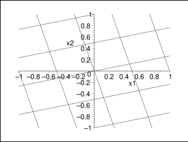
Figure 1: Web corresponding to $K$.

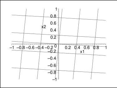
Figure 2: Web corresponding to $\widetilde{K}$.

Since both points $(1,-6,2)$ and $(-4,9,1)$ are in $U_{1}$, we employ the right moving frame $\psi_{1}$ to obtain the following two respective angles

$$\theta_{1}\approx 75\ \mathrm{degrees},\qquad\theta_{2}\approx 4.5\ \mathrm{degrees},$$

which align the orthogonal webs in Figs. 2 and 2 respectively with the coordinate axes for $\mathbb{E}^{2}$. The components of the corresponding canonical forms in $\mathcal{K}^{2}(\mathbb{E}^{2})$ are then

$$K^{ij}\equiv\left(\begin{array}[]{cc}\displaystyle-\frac{5+\sqrt{65}}{2}&0\vspace{2mm}\\ 0&\displaystyle-\frac{5-\sqrt{65}}{2}\end{array}\right),\qquad\widetilde{K}^{ij}\equiv\left(\begin{array}[]{cc}\displaystyle\frac{5-\sqrt{173}}{2}&0\vspace{2mm}\\ 0&\displaystyle\frac{5+\sqrt{173}}{2}\end{array}\right),$$

where the entries of the canonical form for $K$ are the eigenvalues of $K^{ij}$, and the entries of the canonical form for $\widetilde{K}$ are the eigenvalues of $\widetilde{K}^{ij}$, such that in both cases the smaller eigenvalue is in the first row while the larger is in the second row.

Remark 2.9.

Since the components of any other Killing tensor will not have constant eigenvalues for all $(x^{1},x^{2})\in\mathbb{E}^{2}$, Killing tensors with parameters in $E_{1}$ are the only ones which generate Cartesian orthogonal webs.

2.3.3 The 2-dimensional orbits

The Killing tensors associated with points in the invariant submanifold $E_{2}$ generate all the polar webs. In this case, we want a cross-section that corresponds to the polar webs which are aligned with the coordinate axes. Such a regular cross-section is given by

$$\left(\begin{array}[]{cc}\alpha_{1}+\alpha_{6}(x^{2})^{2}&-\alpha_{6}x^{1}x^{2}\vspace{1mm}\\ -\alpha_{6}x^{1}x^{2}&\alpha_{1}+\alpha_{6}(x^{1})^{2}\end{array}\right),\qquad\alpha_{6}\neq 0.$$

The distinguished chart for $E_{2}$ is given below by Table 4.

Table 4: Distinguished chart for $E_{2}\subset\Sigma\simeq\mathbb{R}^{6}$.

0.5ex Chart	Coordinate function	Coordinate neighbourhood 0.5ex
4ex $(U,\varphi)$	$\varphi(\alpha_{1},\ldots,\alpha_{6})=\left(\begin{array}[]{c}\psi(\alpha_{1},\ldots,\alpha_{6})\vspace{1mm}\\ \mathcal{I}_{1}(\alpha_{1},\ldots,\alpha_{6})\vspace{1mm}\\ \mathcal{I}_{2}(\alpha_{1},\ldots,\alpha_{6})\end{array}\right)$	$U=E_{2}$ 4ex

where

$$\displaystyle\psi(\alpha_{1},\ldots,\alpha_{6})=\left(\frac{\alpha_{5}}{\alpha_{6}},\ \frac{\alpha_{4}}{\alpha_{6}}\right),$$

$$\mathcal{I}_{1}(\alpha_{1},\ldots,\alpha_{6})=\alpha_{6}\alpha_{1}-\alpha_{4}^{2},\qquad\mathcal{I}_{2}(\alpha_{1},\ldots,\alpha_{6})=\alpha_{6}.$$ (2.18)

The leaves of this foliation are then

$$L^{2}_{\beta}=\{(\alpha_{1},\ldots,\alpha_{6})\in E_{2}\ |\ \mathcal{I}_{1}(\alpha_{1},\ldots,\alpha_{6})=\beta_{1},\ \mathcal{I}_{2}(\alpha_{1},\ldots,\alpha_{6})=\beta_{2}\},$$ (2.19)

where $\beta_{2}\neq 0$.

Remark 2.10.

For any particular point $(\alpha_{1},\ldots,\alpha_{6})\in E_{2}$, the eigenvalues of the matrix representing the components of the corresponding Killing tensor in $\mathcal{K}^{2}(\mathbb{E}^{2})$ are given by

$$\lambda_{1}=\widetilde{\alpha}_{1},\qquad\lambda_{2}=\widetilde{\alpha}_{1}+\widetilde{\alpha}_{6}\left(\left(x^{1}-\frac{\alpha_{5}}{\alpha_{6}}\right)^{2}+\left(x^{2}-\frac{\alpha_{4}}{\alpha_{6}}\right)^{2}\right),$$ (2.20)

in the sense that the canonical form for the Killing tensor corresponding to that point $(\alpha_{1},\ldots$, $\alpha_{6})\in E_{2}$ is given by

$$\left(\begin{array}[]{cc}\widetilde{\alpha}_{1}+\widetilde{\alpha}_{6}(x^{2})^{2}&-\widetilde{\alpha}_{6}x^{1}x^{2}\vspace{2mm}\\ -\widetilde{\alpha}_{6}x^{1}x^{2}&\widetilde{\alpha}_{1}+\widetilde{\alpha}_{6}(x^{1})^{2}\end{array}\right).$$ (2.23)

Example 2.11.

Consider the following two points in $E_{2}$

$$p_{1}=(\alpha_{1},\ldots,\alpha_{6})=\left(2,1,\tfrac{2}{3},1,2,-3\right),\qquad p_{2}=(\alpha_{1},\ldots,\alpha_{6})=\left(1,-3,\tfrac{8}{3},2,4,-3\right),$$

corresponding respectively to the Killing tensors $K,\widetilde{K}\in\mathcal{K}^{2}(\mathbb{E}^{2})$ with components

$$K^{ij}=\left(\begin{array}[]{cc}2+2x^{2}-3(x^{2})^{2}&\tfrac{2}{3}-x^{1}-2x^{2}+3x^{1}x^{2}\vspace{1mm}\\ \tfrac{2}{3}-x^{1}-2x^{2}+3x^{1}x^{2}&1+4x^{1}-3(x^{1})^{2}\end{array}\right),$$

$$\widetilde{K}^{ij}=\left(\begin{array}[]{cc}1+4x^{2}-3(x^{2})^{2}&\tfrac{8}{3}-2x^{1}-4x^{2}+3x^{1}x^{2}\vspace{1mm}\\ \tfrac{8}{3}-2x^{1}-4x^{2}+3x^{1}x^{2}&-3+8x^{1}-3(x^{1})^{2}\end{array}\right).$$

To determine whether they are $\mathrm{SE}(2)$-equivalent, check which leaf (2.19) each belongs to. Namely, since

$$p_{1}\in L^{2}_{(-7,-3)},\qquad p_{2}\in L^{2}_{(-7,-3)},\qquad\mbox{and}\qquad L^{2}_{(-7,-3)}\equiv L^{2}_{(-7,-3)},$$

the Killing tensors $K$ and $\widetilde{K}$ are $\mathrm{SE}(2)$-equivalent. The transformation to canonical form is best illustrated with the corresponding orthogonal webs. The Killing tensor $K$ generates the orthogonal web in Fig. 4, while the Killing tensor $\widetilde{K}$ generates the orthogonal web in Fig. 4.

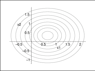
Figure 3: Web corresponding to $K$.

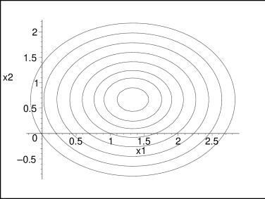
Figure 4: Web corresponding to $\widetilde{K}$.

Employing the right moving frame (2.18) and substituting into the action (2.9) with $\theta=0$ yields the following transformations,

$$\bar{x}^{1}=x^{1}-\tfrac{2}{3},\qquad\bar{x}^{2}=x^{2}-\tfrac{1}{3},$$

which maps the singular point of the orthogonal web in Fig. 4 to the origin, and

$$\bar{x}^{1}=x^{1}-\tfrac{4}{3},\qquad\bar{x}^{2}=x^{2}-\tfrac{2}{3},$$

which maps the singular point of the orthogonal web in Fig. 4 to the origin. Furthermore, utilizing (2.23) and (2.20) yields the components of the canonical form for $K$ and $\widetilde{K}$

$$K\equiv\widetilde{K}\equiv\left(\begin{array}[]{cc}\tfrac{7}{3}-3(x^{2})^{2}&3x^{1}x^{2}\vspace{1mm}\\ 3x^{1}x^{2}&\tfrac{7}{3}-3(x^{1})^{2}\end{array}\right).$$

2.3.4 The 3-dimensional orbits

The Killing tensors that correspond to points in the invariant submanifold $E_{3}$ generate either a parabolic web or an elliptic-hyperbolic web. We may partition $E_{3}$ further by taking advantage of the fact that Killing tensors in $E_{3}$ with $\alpha_{6}=0$ have one singular point, while those in $E_{3}$ with $\alpha_{6}\neq 0$ have two. Namely, set

$$E_{3}^{1}=\{(\alpha_{1},\alpha_{2},\ldots,\alpha_{6})\in E_{3}\ |\ \Delta_{2}=\alpha_{6}=0\},$$

$$E_{3}^{2}=\{(\alpha_{1},\alpha_{2},\ldots,\alpha_{6})\in E_{3}\ |\ \Delta_{2}=\alpha_{6}\neq 0\},$$ (2.24)

so that $E_{3}^{1}$ consists of all parabolic webs and $E_{3}^{2}$ consists of all elliptic-hyperbolic webs.

Parabolic webs. Considering first the family of parabolic webs, we choose a regular cross-section so that the singular point is at the origin and the web is rotationally aligned with the axes. Such a collection of canonical forms is given by,

$$\left(\begin{array}[]{cc}\alpha_{1}&-\alpha_{5}x^{2}\vspace{1mm}\\ -\alpha_{5}x^{2}&\alpha_{1}+2\alpha_{5}x^{1}\end{array}\right),\qquad\alpha_{5}>0.$$ (2.27)

The distinguished charts for $E_{3}^{1}$ is given by Table 5 below.

Table 5: Distinguished charts for $E_{3}^{1}\subset\Sigma\simeq\mathbb{R}^{6}$.

0.5ex Chart	Coordinate function	Coordinate neighbourhood 0.5ex
4ex $(U_{1},\varphi)$	$\varphi(\alpha_{1},\ldots,\alpha_{6})=\left(\begin{array}[]{c}\psi(\alpha_{1},\ldots,\alpha_{6})\\ \mathcal{I}_{1}(\alpha_{1},\ldots,\alpha_{6})\\ \mathcal{I}_{2}(\alpha_{1},\ldots,\alpha_{6})\end{array}\right)$	$U_{1}=\{(\alpha_{1},\ldots,\alpha_{6})\in E_{3}^{1}\ |\ \alpha_{5}>0\}$ 4ex
4ex $(U_{2},\varphi)$	$\varphi(\alpha_{1},\ldots,\alpha_{6})=\left(\begin{array}[]{c}\psi(\alpha_{1},\ldots,\alpha_{6})\\ \mathcal{I}_{1}(\alpha_{1},\ldots,\alpha_{6})\\ \mathcal{I}_{2}(\alpha_{1},\ldots,\alpha_{6})\end{array}\right)$	$U_{2}=\{(\alpha_{1},\ldots,\alpha_{6})\in E_{3}^{1}\ |\ \alpha_{5}<0\}$4ex

where

$$\psi(\alpha_{1},\ldots,\alpha_{6})=\left(\begin{array}[]{c}\theta\\ a\\ b\end{array}\right)=\left(\begin{array}[]{c}-\arctan(\alpha_{4}/\alpha_{5})\vspace{2mm}\\ \displaystyle\frac{\alpha_{5}\sqrt{\frac{\alpha_{4}^{2}+\alpha_{5}^{2}}{\alpha_{5}^{2}}}((\alpha_{1}-\alpha_{2})(\alpha_{4}^{2}-\alpha_{5}^{2})-4\alpha_{3}\alpha_{4}\alpha_{5})}{2(\alpha_{4}^{2}+\alpha_{5}^{2})^{2}}\vspace{2mm}\\ \displaystyle\frac{\alpha_{5}\sqrt{\frac{\alpha_{4}^{2}+\alpha_{5}^{2}}{\alpha_{5}^{2}}}(\alpha_{1}\alpha_{4}\alpha_{5}-\alpha_{2}\alpha_{4}\alpha_{5}-\alpha_{3}\alpha_{5}^{2}+\alpha_{3}\alpha_{4}^{2})}{(\alpha_{4}^{2}+\alpha_{5}^{2})^{2}}\end{array}\right),$$ (2.34)

$$\mathcal{I}_{1}(\alpha_{1},\ldots,\alpha_{6})=\alpha_{4}^{2}+\alpha_{5}^{2},\qquad\mathcal{I}_{2}(\alpha_{1},\ldots,\alpha_{6})=2\alpha_{3}\alpha_{4}\alpha_{5}+\alpha_{1}\alpha_{5}^{2}+\alpha_{2}\alpha_{4}^{2}.$$ (2.35)

In this case, the two families of slices

$$\widetilde{S}^{1}_{\beta}=\{(\alpha_{1},\ldots,\alpha_{6})\in U_{1}\ |\ \mathcal{I}_{1}(\alpha_{1},\ldots,\alpha_{6})=\beta_{1},\mathcal{I}_{2}(\alpha_{1},\ldots,\alpha_{6})=\beta_{2}\},$$

$$\widetilde{S}^{2}_{\beta}=\{(\alpha_{1},\ldots,\alpha_{6})\in U_{2}\ |\ \mathcal{I}_{1}(\alpha_{1},\ldots,\alpha_{6})=\beta_{1},\mathcal{I}_{2}(\alpha_{1},\ldots,\alpha_{6})=\beta_{2}\},$$ (2.36)

must be taken together to form the leaves $\widetilde{L}^{3}_{\beta}$ of the regular foliation. Namely,

$$\widetilde{L}^{3}_{\beta}=\widetilde{S}^{1}_{\beta}\cup\widetilde{S}^{2}_{\beta}$$ (2.37)

for all $(\beta_{1},\beta_{2})\in\mathcal{I}_{1}(E_{3}^{1})\times\mathcal{I}_{2}(E_{3}^{1})$.

Consult Table 6 for the moving frame that maps an arbitrary element in $E_{3}^{1}$ to the cross-section (2.27). See (2.35) for $(\theta,a,b)$.

Table 6: Right moving frame for the global regular cross-section (2.27).

0.5ex Coordinate neighbourhood	Right moving frame:
	See (2.35) for $(\theta,a,b)$ 0.5ex
3ex $(\alpha_{1},\ldots,\alpha_{6})\in U_{1}$	$\left(\!\!\begin{array}[]{c}\theta\\ a\\ b\end{array}\!\!\right)$ 3ex
3ex $(\alpha_{1},\ldots,\alpha_{6})\in U_{2}$	$\left(\!\!\begin{array}[]{c}\theta\pm\pi\\ -a\\ -b\end{array}\!\!\right)$ 3ex

In addition, the canonical form for an arbitrary point in $E_{3}^{1}$ may be determined by the invariant functions (2.35). That is, the components of the canonical form for a Killing tensor corresponding to an arbitrary point in $E_{3}^{1}$ is given by

$$\left(\begin{array}[]{cc}\displaystyle\frac{\mathcal{I}_{2}}{\mathcal{I}_{1}}&-\sqrt{\mathcal{I}_{1}}x^{2}\vspace{1mm}\\ -\sqrt{\mathcal{I}_{1}}x^{2}&\displaystyle\frac{\mathcal{I}_{2}}{\mathcal{I}_{1}}+2\sqrt{\mathcal{I}_{1}}x^{1}\end{array}\right).$$ (2.40)

Example 2.12.

Consider the following two points in $E_{3}^{1}$

$$p_{1}=(\alpha_{1},\ldots,\alpha_{6})=(1,-3,5,1,2,0),\qquad p_{2}=(\alpha_{1},\ldots,\alpha_{6})=(-2,5,7,0,-1,0),$$

corresponding respectively to the Killing tensors $K$ and $\widetilde{K}$ with components

$$K^{ij}=\left(\begin{array}[]{cc}2+2x^{2}-3(x^{2})^{2}&\tfrac{2}{3}-x^{1}-2x^{2}+3x^{1}x^{2}\vspace{1mm}\\ \tfrac{2}{3}-x^{1}-2x^{2}+3x^{1}x^{2}&1+4x^{1}-3(x^{1})^{2}\end{array}\right),$$

$$\widetilde{K}^{ij}=\left(\begin{array}[]{cc}1+4x^{2}-3(x^{2})^{2}&\tfrac{8}{3}-2x^{1}-4x^{2}+3x^{1}x^{2}\vspace{1mm}\\ \tfrac{8}{3}-2x^{1}-4x^{2}+3x^{1}x^{2}&-3+8x^{1}-3(x^{1})^{2}\end{array}\right).$$

To determine whether $K$ and $\widetilde{K}$ belong to the same equivalence class, utilize (2.36) and (2.37) to find out which leaf each belongs to. Namely, since

$$p_{1}\in\widetilde{L}^{3}_{(5,21)},\hskip 28.45274ptp_{2}\in\widetilde{L}^{3}_{(1,-2)},\qquad\mbox{and}\qquad\widetilde{L}^{3}_{(5,21)}\not\equiv\widetilde{L}^{3}_{(1,-2)},$$

the Killing tensors $K$ and $\widetilde{K}$ are not $\mathrm{SE}(2)$-equivalent. To illustrate the transformation to canonical form, consider the web generated by $K$ (see Fig. 6) and the web generated by $\widetilde{K}$ (see Fig. 6).

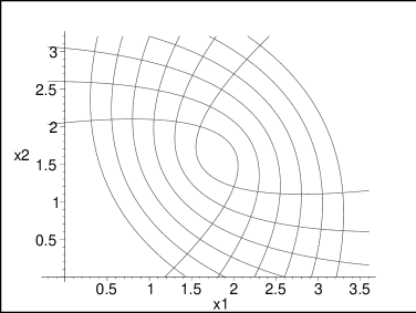
Figure 5: Web corresponding to $K$.

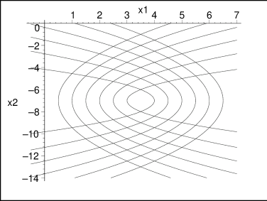
Figure 6: Web corresponding to $\widetilde{K}$.

The right moving frame from Table 6 immediately tells us that the map which takes the web in Fig. 6 to its canonical form requires the following rotation and translation

$$\theta=-\arctan\left(\tfrac{1}{2}\right)\ \mathrm{radians}\approx-27\ \mathrm{degrees},\qquad a=-\tfrac{26\sqrt{5}}{25},\qquad b=-\tfrac{7\sqrt{5}}{25},$$ (2.41)

where $a$ is a horizontal translation and $b$ is a vertical translation (applied after the rotation). Substituting (2.41) into the action (2.9) yields the following transformation

$$\bar{x}^{1}=\tfrac{2}{\sqrt{5}}x^{1}+\tfrac{1}{\sqrt{5}}x^{2}-\tfrac{26\sqrt{5}}{25},\qquad\bar{x}^{2}=-\tfrac{1}{\sqrt{5}}x^{1}+\tfrac{2}{\sqrt{5}}x^{2}-\tfrac{7\sqrt{5}}{25},$$

which maps the singular point to the origin and aligns the web from Fig. 6 with the coordinate axes for the ambient manifold $\mathbb{E}^{2}$. Similarly, applying the right moving frame to the web in Fig. 6 yields the following rotation and translation

$$\theta=\pm\ \pi\ \mathrm{radians},\qquad a=\tfrac{7}{2},\qquad b=-7.$$ (2.42)

Substituting (2.42) into the action (2.9) then gives the following transformation

$$\bar{x}^{1}=-x^{1}+\tfrac{7}{2},\qquad\bar{x}^{2}=-x^{2}-7,$$

which maps the singular point to the origin and aligns the web from Fig. 6 with the coordinate axes for the ambient manifold $\mathbb{E}^{2}$.

Implementing formula (2.40) gives the following canonical forms on the cross-section (2.27) for the components of the associated Killing tensors $K$ and $\widetilde{K}$

$$\begin{array}[]{l}K^{ij}\equiv\left(\begin{array}[]{cc}\displaystyle\tfrac{21}{5}&-\sqrt{5}x^{2}\vspace{1mm}\\ -\sqrt{5}x^{2}&\displaystyle\tfrac{21}{5}+2\sqrt{5}x^{1}\end{array}\right),\qquad\widetilde{K}^{ij}\equiv\left(\begin{array}[]{cc}-2&-x^{2}\\ \vskip 6.0pt plus 2.0pt minus 2.0pt\cr-x^{2}&-2+2x^{1}\end{array}\right).\end{array}$$

Elliptic-hyperbolic webs. For the family of elliptic-hyperbolic webs, the canonical forms should be those webs aligned with the coordinate axes for the ambient manifold $\mathbb{E}^{2}$. That is, we choose those webs whose singular points are on the horizontal axis and equi-distant from the origin. In this regard, the regular cross-section

$$\left(\begin{array}[]{cc}\alpha_{1}+\alpha_{6}(x^{2})^{2}&-\alpha_{6}x^{1}x^{2}\\ -\alpha_{6}x^{1}x^{2}&\alpha_{2}+\alpha_{6}(x^{1})^{2}\end{array}\right),\qquad\alpha_{6}(\alpha_{1}-\alpha_{2})>0,$$ (2.45)

satisfies the desired criteria.

The distinguished charts for the invariant submanifold $E_{3}^{2}$ is given by Table 7 below.

Table 7: Distinguished charts for $E_{3}^{2}\subset\Sigma\simeq\mathbb{R}^{6}$.

0.5ex$\iota_{1}=\alpha_{6}(\alpha_{1}-\alpha_{2})-\alpha_{4}^{2}+\alpha_{5}^{2}$,   $\iota_{2}=\alpha_{3}\alpha_{6}+\alpha_{4}\alpha_{5}$0.5ex
0.5ex Chart	Coordinate function	Coordinate Neighbourhood 0.5ex
5ex $(U_{1},\varphi)$	$\varphi(\alpha_{1},\ldots,\alpha_{6})=\left(\begin{array}[]{c}\psi_{1}(\alpha_{1},\ldots,\alpha_{6})\\ \mathcal{I}_{1}(\alpha_{1},\ldots,\alpha_{6})\\ \mathcal{I}_{2}(\alpha_{1},\ldots,\alpha_{6})\\ \mathcal{I}_{3}(\alpha_{1},\ldots,\alpha_{6})\end{array}\right)$	$U_{1}=\{(\alpha_{1},\ldots,\alpha_{6})\in E_{3}^{2}\ |\ \iota_{1}>0\}$ 5ex
5ex $(U_{2},\varphi)$	$\varphi(\alpha_{1},\ldots,\alpha_{6})=\left(\begin{array}[]{c}\psi_{1}(\alpha_{1},\ldots,\alpha_{6})\\ \mathcal{I}_{1}(\alpha_{1},\ldots,\alpha_{6})\\ \mathcal{I}_{2}(\alpha_{1},\ldots,\alpha_{6})\\ \mathcal{I}_{3}(\alpha_{1},\ldots,\alpha_{6})\end{array}\right)$	$U_{2}=\{(\alpha_{1},\ldots,\alpha_{6})\in E_{3}^{2}\ |\ \iota_{1}<0\}$5ex
5ex $(U_{3},\widetilde{\varphi})$	$\varphi(\alpha_{1},\ldots,\alpha_{6})=\left(\begin{array}[]{c}\psi_{2}(\alpha_{1},\ldots,\alpha_{6})\\ \mathcal{I}_{1}(\alpha_{1},\ldots,\alpha_{6})\\ \mathcal{I}_{2}(\alpha_{1},\ldots,\alpha_{6})\\ \mathcal{I}_{3}(\alpha_{1},\ldots,\alpha_{6})\end{array}\right)$	$U_{3}=\{(\alpha_{1},\ldots,\alpha_{6})\in E_{3}^{2}\ |\ \iota_{2}>0\}$ 5ex
5ex $(U_{4},\widetilde{\varphi})$	$\varphi(\alpha_{1},\ldots,\alpha_{6})=\left(\begin{array}[]{c}\psi_{2}(\alpha_{1},\ldots,\alpha_{6})\\ \mathcal{I}_{1}(\alpha_{1},\ldots,\alpha_{6})\\ \mathcal{I}_{2}(\alpha_{1},\ldots,\alpha_{6})\\ \mathcal{I}_{3}(\alpha_{1},\ldots,\alpha_{6})\end{array}\right)$	$U_{4}=\{(\alpha_{1},\ldots,\alpha_{6})\in E_{3}^{2}\ |\ \iota_{2}<0\}$ 5ex

where

$$\psi_{1}(\alpha_{1},\ldots,\alpha_{6})=\left(\begin{array}[]{c}\theta_{1}\\ a_{1}\\ b_{1}\\ \end{array}\right)=\left(\begin{array}[]{c}\displaystyle-\frac{1}{2}\arctan\left(\frac{2(\alpha_{3}\alpha_{6}+\alpha_{4}\alpha_{5})}{\alpha_{6}(\alpha_{1}-\alpha_{2})-\alpha_{4}^{2}+\alpha_{5}^{2}}\right)\vspace{1mm}\\ \displaystyle\frac{\alpha_{5}\cos\theta_{1}-\alpha_{4}\sin\theta_{1}}{\alpha_{6}}\vspace{1mm}\\ \displaystyle\frac{\alpha_{4}\cos\theta_{1}+\alpha_{5}\sin\theta_{1}}{\alpha_{6}}\end{array}\right),$$ (2.52)

$$\psi_{2}(\alpha_{1},\ldots,\alpha_{6})=\left(\begin{array}[]{c}\theta_{2}\\ a_{2}\\ b_{2}\end{array}\right)=\left(\begin{array}[]{c}\displaystyle\frac{1}{2}\arctan\left(\frac{\alpha_{6}(\alpha_{1}-\alpha_{2})-\alpha_{4}^{2}+\alpha_{5}^{2}}{2(\alpha_{3}\alpha_{6}+\alpha_{4}\alpha_{5})}\right)\vspace{1mm}\\ \displaystyle\frac{\alpha_{5}\cos\theta_{2}-\alpha_{4}\sin\theta_{2}}{\alpha_{6}}\vspace{1mm}\\ \displaystyle\frac{\alpha_{4}\cos\theta_{2}+\alpha_{5}\sin\theta_{2}}{\alpha_{6}}\end{array}\right),$$ (2.59)

$$\mathcal{I}_{1}(\alpha_{1},\ldots,\alpha_{6})=\alpha_{6},\qquad\mathcal{I}_{2}(\alpha_{1},\ldots,\alpha_{6})=\alpha_{6}(\alpha_{1}+\alpha_{2})-\alpha_{4}^{2}-\alpha_{5}^{2},$$

$$\mathcal{I}_{3}(\alpha_{1},\ldots,\alpha_{6})=\alpha_{6}(\alpha_{3}^{2}-\alpha_{1}\alpha_{2})+\alpha_{4}^{2}\alpha_{2}+2\alpha_{3}\alpha_{4}\alpha_{5}+\alpha_{1}\alpha_{5}^{2}.$$

Each leaf of the regular foliation is a union of the slices

$$S^{1}_{\beta}=\{(\alpha_{1},\ldots,\alpha_{6})\in U_{1}\ |\ \mathcal{I}_{1}=\beta_{1},\mathcal{I}_{2}=\beta_{2},\mathcal{I}_{3}=\beta_{3}\},$$

$$S^{2}_{\beta}=\{(\alpha_{1},\ldots,\alpha_{6})\in U_{2}\ |\ \mathcal{I}_{1}=\beta_{1},\mathcal{I}_{2}=\beta_{2},\mathcal{I}_{3}=\beta_{3}\},$$

$$S^{3}_{\beta}=\{(\alpha_{1},\ldots,\alpha_{6})\in U_{3}\ |\ \mathcal{I}_{1}=\beta_{1},\mathcal{I}_{2}=\beta_{2},\mathcal{I}_{3}=\beta_{3}\},$$

$$S^{4}_{\beta}=\{(\alpha_{1},\ldots,\alpha_{6})\in U_{4}\ |\ \mathcal{I}_{1}=\beta_{1},\mathcal{I}_{2}=\beta_{2},\mathcal{I}_{3}=\beta_{3}\},$$ (2.60)

In particular, the leaves, indexed by all $\beta=(\beta_{1},\beta_{2},\beta_{3})$ in $\mathcal{I}_{1}(E_{3}^{2})\times\mathcal{I}_{2}(E_{3}^{2})\times\mathcal{I}_{3}(E_{3}^{2})$, are given by

$$L^{3}_{\beta}=\bigcup_{i=1}^{4}S^{i}_{\beta}.$$ (2.61)

For the right moving frame giving the transformation that takes a Killing tensor to its canonical form (2.45), consult Table 8 below.

Table 8: Right moving frame for the global regular cross-section (2.45).

0.5ex	Right moving frame:
Coordinate neighbourhood	see (2.59) for $(\theta_{i},a_{i},b_{i})$, $i=1,2$ 0.5ex
4ex $(\alpha_{1},\ldots,\alpha_{6})\in U_{1}$	$\displaystyle\left(\begin{array}[]{c}\theta\\ a\\ b\end{array}\right)=\left(\begin{array}[]{c}\theta_{1}\\ a_{1}\\ b_{1}\end{array}\right)$ 4ex
4ex $(\alpha_{1},\ldots,\alpha_{6})\in U_{2}$	$\displaystyle\left(\begin{array}[]{c}\theta\\ a\\ b\end{array}\right)=\left(\begin{array}[]{c}\theta_{1}\pm\pi/2\\ \mp b_{1}\\ \pm a_{1}\end{array}\right)$ 4ex
4ex $(\alpha_{1},\ldots,\alpha_{6})\in U_{3}$	$\displaystyle\left(\begin{array}[]{c}\theta\\ a\\ b\end{array}\right)=\left(\begin{array}[]{c}\theta_{2}-\pi/4\\ \displaystyle\frac{a_{2}}{\sqrt{2}}+\frac{b_{2}}{\sqrt{2}}\\ \displaystyle-\frac{a_{2}}{\sqrt{2}}+\frac{b_{2}}{\sqrt{2}}\end{array}\right)$ 4ex
4ex $(\alpha_{1},\ldots,\alpha_{6})\in U_{4}$	$\displaystyle\left(\begin{array}[]{c}\theta\\ a\\ b\end{array}\right)=\left(\begin{array}[]{c}\theta_{2}+\pi/4\\ \displaystyle\frac{a_{2}}{\sqrt{2}}-\frac{b_{2}}{\sqrt{2}}\\ \displaystyle\frac{a_{2}}{\sqrt{2}}+\frac{b_{2}}{\sqrt{2}}\end{array}\right)$ 4ex

Moreover, the formula for the canonical form of an arbitrary point in $E_{3}^{2}$ is

$$P^{+}=\left(\frac{\mathcal{I}_{2}}{2\mathcal{I}_{1}}+\sqrt{\frac{\mathcal{I}_{3}}{\mathcal{I}_{1}}+\left(\frac{\mathcal{I}_{2}}{2\mathcal{I}_{1}}\right)^{2}},\ \frac{\mathcal{I}_{2}}{2\mathcal{I}_{1}}-\sqrt{\frac{\mathcal{I}_{3}}{\mathcal{I}_{1}}+\left(\frac{\mathcal{I}_{2}}{2\mathcal{I}_{1}}\right)^{2}},0,0,0,\mathcal{I}_{1}\right),$$ (2.62)

whenever $\mathcal{I}_{1}>0$, and the point

$$P^{-}=\left(\frac{\mathcal{I}_{2}}{2\mathcal{I}_{1}}-\sqrt{\frac{\mathcal{I}_{3}}{\mathcal{I}_{1}}+\left(\frac{\mathcal{I}_{2}}{2\mathcal{I}_{1}}\right)^{2}},\ \frac{\mathcal{I}_{2}}{2\mathcal{I}_{1}}+\sqrt{\frac{\mathcal{I}_{3}}{\mathcal{I}_{1}}+\left(\frac{\mathcal{I}_{2}}{2\mathcal{I}_{1}}\right)^{2}},0,0,0,\mathcal{I}_{1}\right),$$ (2.63)

whenever $\mathcal{I}_{1}<0$.

Example 2.13.

Consider the following two points in $E_{3}^{2}$

$$p_{1}=(\alpha_{1},\ldots,\alpha_{6})=(2,1,0,1,1,4),\qquad p_{2}=(\alpha_{1},\ldots,\alpha_{6})=(2,1,0,1,1,-4),$$

corresponding respectively to the Killing tensors $K$ and $\widetilde{K}$ with components

$$K^{ij}=\left(\begin{array}[]{cc}2+2x^{2}+4(x^{2})^{2}&-x^{1}-x^{2}-4x^{1}x^{2}\vspace{1mm}\\ -x^{1}-x^{2}-4x^{1}x^{2}&1+2x^{1}+4(x^{1})^{2}\end{array}\right),$$

$$\widetilde{K}^{ij}=\left(\begin{array}[]{cc}2+2x^{2}-4(x^{2})^{2}&-x^{1}-x^{2}+4x^{1}x^{2}\vspace{1mm}\\ -x^{1}-x^{2}+4x^{1}x^{2}&1+2x^{1}-4(x^{1})^{2}\end{array}\right).$$

To determine whether $K$ and $\widetilde{K}$ are $\mathrm{SE}(2)$-equivalent, use the formulae (2.60) for the slices to ascertain which leaf, using (2.61), each belongs to. That is to say, since

$$p_{1}\in L^{3}_{(4,10,-5)},\qquad p_{2}\in L^{3}_{(-4,-14,11)},\qquad\mbox{and}\qquad L^{3}_{(4,10,-5)}\not\equiv L^{3}_{(-4,-14,11)},$$

the Killing tensors $K$ and $\widetilde{K}$ are not $\mathrm{SE}(2)$-equivalent. To illustrate the transformation to canonical form, it is useful to regard the corresponding orthogonal webs. See Fig. 8 for the web generated by $K$ and Fig. 8 for the web generated by $\widetilde{K}$.

Figure 7: Web corresponding to $K$.

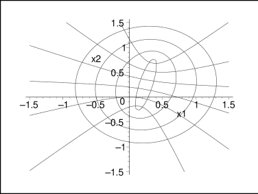
Figure 8: Web corresponding to $\widetilde{K}$.

Consulting Table 7 will reveal that $p_{1}\in U_{1}$ and $p_{2}\in U_{3}$. Table 8 gives the appropriate right moving frame for each point. Namely, for $p_{1}$ (the web in Fig. 8)

$$\theta=-\tfrac{1}{2}\arctan\left(\tfrac{1}{2}\right)\ \mathrm{radians}\approx-13\ \mathrm{degrees},$$

$$a=\tfrac{1}{4}\cos\left(\tfrac{1}{2}\arctan\left(\tfrac{1}{2}\right)\right)+\tfrac{1}{4}\sin\left(\tfrac{1}{2}\arctan\left(\tfrac{1}{2}\right)\right)\approx 0.30,$$

$$b=\tfrac{1}{4}\cos\left(\tfrac{1}{2}\arctan\left(\tfrac{1}{2}\right)\right)-\tfrac{1}{4}\sin\left(\tfrac{1}{2}\arctan\left(\tfrac{1}{2}\right)\right)\approx 0.18.$$ (2.64)

Substituting (2.64) into the action (2.9) gives the transformation

$$\bar{x}^{1}=x^{1}\cos\left(\tfrac{1}{2}\arctan\left(\tfrac{1}{2}\right)\right)+x^{2}\sin\left(\tfrac{1}{2}\arctan\left(\tfrac{1}{2}\right)\right)$$

$$\phantom{\bar{x}^{1}=}{}+\tfrac{1}{4}\cos\left(\tfrac{1}{2}\arctan\left(\tfrac{1}{2}\right)\right)+\tfrac{1}{4}\sin\left(\tfrac{1}{2}\arctan\left(\tfrac{1}{2}\right)\right),$$

$$\bar{x}^{2}=-x^{1}\sin\left(\tfrac{1}{2}\arctan\left(\tfrac{1}{2}\right)\right)+x^{2}\cos\left(\tfrac{1}{2}\arctan\left(\tfrac{1}{2}\right)\right)$$

$$\phantom{\bar{x}^{2}=}{}+\tfrac{1}{4}\cos\left(\tfrac{1}{2}\arctan\left(\tfrac{1}{2}\right)\right)-\tfrac{1}{4}\sin\left(\tfrac{1}{2}\arctan\left(\tfrac{1}{2}\right)\right),$$

which maps the singular points (foci) in Fig. 8 to the $x^{1}$-axis so that they are equally distant from the origin. Similarly, consulting Table 8 we get for $p_{2}$ (the web in Fig. 8)

$$\theta=-\tfrac{1}{2}\arctan(2)-\tfrac{\pi}{4}\ \mathrm{radians}\approx-77\ \mathrm{degrees},$$ (2.65)

$$a=-\tfrac{\sqrt{2}}{4}\cos\left(\tfrac{1}{2}\arctan(2)\right)\approx-0.30,\qquad b=\tfrac{\sqrt{2}}{4}\sin\left(\tfrac{1}{2}\arctan(2)\right)\approx 0.18.$$

Substituting (2.65) into the action (2.9) gives the transformation

$$\bar{x}^{1}=\cos\left(\frac{\arctan(2)}{2}\right)\left(\frac{x^{1}+x^{2}}{\sqrt{2}}-\frac{1}{2\sqrt{2}}\right)+\sin\left(\frac{\arctan(2)}{2}\right)\left(\frac{-x^{1}+x^{2}}{\sqrt{2}}\right),$$

$$\bar{x}^{2}=\cos\left(\frac{\arctan(2)}{2}\right)\left(\frac{-x^{1}+x^{2}}{\sqrt{2}}\right)+\sin\left(\frac{\arctan(2)}{2}\right)\left(\frac{-x^{1}-x^{2}}{\sqrt{2}}+\frac{1}{2\sqrt{2}}\right),$$

mapping the singular points (foci) in Fig. 8 to the $x^{1}$-axis so that they are equally distant from the origin.

In order to determine the canonical form for both $p_{1}$ and $p_{2}$, simply appeal to (2.62) and (2.63). The resulting canonical forms are

$$p_{1}\equiv\left(\frac{5+\sqrt{5}}{4},\frac{5-\sqrt{5}}{4},0,0,0,4\right),\hskip 28.45274ptp_{2}\equiv\left(\frac{7-\sqrt{5}}{4},\frac{7+\sqrt{5}}{4},0,0,0,-4\right),$$

which correspond to Killing tensors that generate elliptic-hyperbolic webs with singular values on the $x^{1}$-axis equally distant from the origin in $\mathbb{E}^{2}$.

2.4 The $\boldsymbol{\mathrm{SE}(3)}$-equivalence of Killing two-tensors

The components of a general Killing two-tensor defined in Euclidean space are given by

$$K_{11}=A_{{1}}-2\,B_{{1,2}}x^{3}+2\,B_{{1,3}}x^{2}+C_{{2}}{(x^{3})}^{2}+C_{{3}}{(x^{2})}^{2}-2\,\gamma_{{1}}x^{2}x^{3},$$

$$K_{22}=A_{{2}}-2\,B_{{2,3}}x^{1}+2\,B_{{2,1}}x^{3}+C_{{3}}{(x^{1})}^{2}+C_{{1}}{(x^{3})}^{2}-2\,\gamma_{{2}}x^{3}x^{1},$$

$$K_{33}=A_{{3}}-2\,B_{{3,1}}x^{2}+2\,B_{{3,2}}x^{1}+C_{{1}}{(x^{2})}^{2}+C_{{2}}{(x^{1})}^{2}-2\,\gamma_{{3}}x^{1}x^{2},$$

$$K_{23}=\alpha_{{1}}+B_{{3,1}}x^{3}-B_{{2,1}}x^{2}+\beta_{1}x^{1}+\left(\gamma_{{3}}x^{3}+\gamma_{{2}}x^{2}-\gamma_{{1}}x^{1}\right)x^{1}-C_{{1}}x^{2}x^{3},$$

$$K_{31}=\alpha_{{2}}+B_{{1,2}}x^{1}-B_{{3,2}}x^{3}+\beta_{2}x^{2}+\left(\gamma_{{1}}x^{1}+\gamma_{{3}}x^{3}-\gamma_{{2}}x^{2}\right)x^{2}-C_{{2}}x^{3}x^{1},$$

$$K_{12}=\alpha_{{3}}+B_{{2,3}}x^{2}-B_{{1,3}}x^{1}-\left(\beta_{1}+\beta_{2}\right)x^{3}+\left(\gamma_{{2}}x^{2}+\gamma_{{1}}x^{1}-\gamma_{{3}}x^{3}\right)x^{3}-C_{{3}}x^{1}x^{2}.$$ (2.66)

The $\mathrm{SE}(3)$ equivalence problem on these Killing tensors concerns the action of a $6$-dimensional group acting on a $20$-dimensional vector space. As a result, any explicit representation of the induced action on the twenty parameters defining a Killing-two tensor will be very large. To obtain such a representation, we must first consider the action of the proper Euclidean group for $\mathbb{E}^{3}$, mapping a point $(x^{1},x^{2},x^{3})\in\mathbb{E}^{3}$ to

$$\bar{x}^{1}=\cos\left(\theta_{{{x}^{3}}}\right)\cos\left(\theta_{{{x}^{2}}}\right)x^{1}+\cos\left(\theta_{{{x}^{3}}}\right)\sin\left(\theta_{{{x}^{2}}}\right)\sin\left(\theta_{{x^{1}}}\right){x}^{2}+\cos\left(\theta_{{{x}^{3}}}\right)\sin\left(\theta_{{{x}^{2}}}\right)\cos\left(\theta_{{x^{1}}}\right){x}^{3}$$

$$\phantom{\bar{x}^{1}=}{}-\sin\left(\theta_{{{x}^{3}}}\right)\cos\left(\theta_{{x^{1}}}\right){x}^{2}+\sin\left(\theta_{{{x}^{3}}}\right)\sin\left(\theta_{{x^{1}}}\right){x}^{3}+a,$$

$$\bar{x}^{2}=\sin\left(\theta_{{{x}^{3}}}\right)\cos\left(\theta_{{{x}^{2}}}\right)x^{1}+\sin\left(\theta_{{{x}^{3}}}\right)\sin\left(\theta_{{{x}^{2}}}\right)\sin\left(\theta_{{x^{1}}}\right){x}^{2}+\sin\left(\theta_{{{x}^{3}}}\right)\sin\left(\theta_{{{x}^{2}}}\right)\cos\left(\theta_{{x^{1}}}\right){x}^{3}$$

$$\phantom{\bar{x}^{2}=}{}+\cos\left(\theta_{{{x}^{3}}}\right)\cos\left(\theta_{{x^{1}}}\right){x}^{2}-\cos\left(\theta_{{{x}^{3}}}\right)\sin\left(\theta_{{x^{1}}}\right){x}^{3}+b,$$

$$\bar{x}^{3}=-\sin\left(\theta_{{{x}^{2}}}\right)x+\cos\left(\theta_{{{x}^{2}}}\right)\left(\sin\left(\theta_{{x^{1}}}\right){x}^{2}+\cos\left(\theta_{{x^{1}}}\right){x}^{3}\right)+c.$$ (2.67)

This particular representation is given by first rotating about the $x^{3}$-axis $(\theta_{x^{3}})$, followed by the $x^{2}$-axis $(\theta_{x^{2}})$ and ending with the rotation about the $x^{1}$-axis $(\theta_{x^{1}})$. In this case, the group parameters are given by $(\theta_{x^{1}},\theta_{x^{2}},\theta_{x^{3}},a,b,c)$.

To obtain the corresponding action on the parameters of $\mathcal{K}^{2}(\mathbb{E}^{3})$, we must determine the effect of the push forward for (2.67) on the components $K^{ij}$ (2.66). Such an action has been computed, however due to sheer size it cannot appear here. In order to illustrate, we have that the parameter $B_{1,3}$ transforms like

$$\overline{B_{1,3}}=C_{{1}}b\left(\cos\left(\theta_{{{x}^{2}}}\right)\right)^{2}-C_{{2}}\left(\cos\left(\theta_{{{x}^{2}}}\right)\right)^{2}b-B_{{2,1}}\sin\left(\theta_{{x^{1}}}\right)\cos\left(\theta_{{{x}^{3}}}\right)-B_{{3,1}}\cos\left(\theta_{{x^{1}}}\right)\cos\left(\theta_{{{x}^{3}}}\right)$$

$$\phantom{\overline{B_{1,3}}=}{}+B_{{3,2}}\cos\left(\theta_{{{x}^{2}}}\right)\sin\left(\theta_{{{x}^{3}}}\right)-C_{{1}}\cos\left(\theta_{{{x}^{2}}}\right)c\sin\left(\theta_{{{x}^{2}}}\right)\sin\left(\theta_{{{x}^{3}}}\right)$$

$$\phantom{\overline{B_{1,3}}=}{}-B_{{3,2}}\cos\left(\theta_{{{x}^{2}}}\right)\sin\left(\theta_{{{x}^{3}}}\right)\left(\cos\left(\theta_{{x^{1}}}\right)\right)^{2}+B_{{3,1}}\cos\left(\theta_{{x^{1}}}\right)\cos\left(\theta_{{{x}^{3}}}\right)\left(\cos\left(\theta_{{{x}^{2}}}\right)\right)^{2}$$

$$\phantom{\overline{B_{1,3}}=}{}+B_{{2,1}}\sin\left(\theta_{{x^{1}}}\right)\cos\left(\theta_{{{x}^{3}}}\right)\left(\cos\left(\theta_{{{x}^{2}}}\right)\right)^{2}+C_{{2}}\cos\left(\theta_{{{x}^{2}}}\right)\sin\left(\theta_{{{x}^{3}}}\right)\sin\left(\theta_{{{x}^{2}}}\right)c$$

$$\phantom{\overline{B_{1,3}}=}{}+2\gamma_{{2}}\left(\cos\left(\theta_{{{x}^{2}}}\right)\right)^{2}\sin\left(\theta_{{{x}^{3}}}\right)\cos\left(\theta_{{x^{1}}}\right)c+\gamma_{{2}}\sin\left(\theta_{{x^{1}}}\right)\cos\left(\theta_{{{x}^{3}}}\right)\sin\left(\theta_{{{x}^{2}}}\right)c$$

$$\phantom{\overline{B_{1,3}}=}{}+2\gamma_{{1}}\sin\left(\theta_{{x^{1}}}\right)\cos\left(\theta_{{{x}^{2}}}\right)c\cos\left(\theta_{{x^{1}}}\right)\sin\left(\theta_{{{x}^{2}}}\right)\sin\left(\theta_{{{x}^{3}}}\right)$$

$$\phantom{\overline{B_{1,3}}=}{}+2\gamma_{{1}}\left(\cos\left(\theta_{{x^{1}}}\right)\right)^{2}\cos\left(\theta_{{{x}^{3}}}\right)\cos\left(\theta_{{{x}^{2}}}\right)c-C_{{3}}\sin\left(\theta_{{x^{1}}}\right)\cos\left(\theta_{{{x}^{2}}}\right)c\cos\left(\theta_{{x^{1}}}\right)\cos\left(\theta_{{{x}^{3}}}\right)$$

$$\phantom{\overline{B_{1,3}}=}{}-\gamma_{{3}}\sin\left(\theta_{{{x}^{2}}}\right)c\cos\left(\theta_{{x^{1}}}\right)\cos\left(\theta_{{{x}^{3}}}\right)-C_{{2}}\left(\cos\left(\theta_{{x^{1}}}\right)\right)^{2}\cos\left(\theta_{{{x}^{2}}}\right)c\sin\left(\theta_{{{x}^{2}}}\right)\sin\left(\theta_{{{x}^{3}}}\right)$$

$$\phantom{\overline{B_{1,3}}=}{}+B_{{2,3}}\cos\left(\theta_{{{x}^{2}}}\right)\cos\left(\theta_{{x^{1}}}\right)\sin\left(\theta_{{{x}^{2}}}\right)\cos\left(\theta_{{{x}^{3}}}\right)\sin\left(\theta_{{x^{1}}}\right)$$

$$\phantom{\overline{B_{1,3}}=}{}+C_{{3}}\cos\left(\theta_{{{x}^{2}}}\right)\sin\left(\theta_{{{x}^{3}}}\right)\sin\left(\theta_{{{x}^{2}}}\right)c\left(\cos\left(\theta_{{x^{1}}}\right)\right)^{2}+2\,\gamma_{{3}}\left(\cos\left(\theta_{{{x}^{2}}}\right)\right)^{2}\sin\left(\theta_{{{x}^{3}}}\right)\sin\left(\theta_{{x^{1}}}\right)c$$

$$\phantom{\overline{B_{1,3}}=}{}+C_{{2}}\sin\left(\theta_{{x^{1}}}\right)\cos\left(\theta_{{{x}^{2}}}\right)c\cos\left(\theta_{{x^{1}}}\right)\cos\left(\theta_{{{x}^{3}}}\right)+\left(\cos\left(\theta_{{{x}^{2}}}\right)\right)^{2}\cos\left(\theta_{{{x}^{3}}}\right)B_{{1,3}}\cos\left(\theta_{{x^{1}}}\right)$$

$$\phantom{\overline{B_{1,3}}=}{}+B_{{3,2}}\cos\left(\theta_{{{x}^{2}}}\right)\cos\left(\theta_{{x^{1}}}\right)\sin\left(\theta_{{{x}^{2}}}\right)\cos\left(\theta_{{{x}^{3}}}\right)\sin\left(\theta_{{x^{1}}}\right)$$

$$\phantom{\overline{B_{1,3}}=}{}-\beta_{{1}}\cos\left(\theta_{{{x}^{2}}}\right)\sin\left(\theta_{{{x}^{2}}}\right)\cos\left(\theta_{{{x}^{3}}}\right)\left(\cos\left(\theta_{{x^{1}}}\right)\right)^{2}-\beta_{{1}}\cos\left(\theta_{{{x}^{2}}}\right)\sin\left(\theta_{{{x}^{3}}}\right)\sin\left(\theta_{{x^{1}}}\right)\cos\left(\theta_{{x^{1}}}\right)$$

$$\phantom{\overline{B_{1,3}}=}{}-2\left(\cos\left(\theta_{{{x}^{2}}}\right)\right)^{2}\gamma_{{1}}b\sin\left(\theta_{{x^{1}}}\right)\cos\left(\theta_{{x^{1}}}\right)+2\gamma_{{3}}\cos\left(\theta_{{{x}^{2}}}\right)b\sin\left(\theta_{{x^{1}}}\right)\sin\left(\theta_{{{x}^{2}}}\right)$$

$$\phantom{\overline{B_{1,3}}=}{}+2\cos\left(\theta_{{{x}^{2}}}\right)\gamma_{{2}}b\sin\left(\theta_{{{x}^{2}}}\right)\cos\left(\theta_{{x^{1}}}\right)-C_{{3}}\left(\cos\left(\theta_{{{x}^{2}}}\right)\right)^{2}b\left(\cos\left(\theta_{{x^{1}}}\right)\right)^{2}$$

$$\phantom{\overline{B_{1,3}}=}{}-\gamma_{{2}}\sin\left(\theta_{{{x}^{3}}}\right)c\cos\left(\theta_{{x^{1}}}\right)-\gamma_{{3}}c\sin\left(\theta_{{x^{1}}}\right)\sin\left(\theta_{{{x}^{3}}}\right)-B_{{3,1}}\sin\left(\theta_{{x^{1}}}\right)\sin\left(\theta_{{{x}^{2}}}\right)\sin\left(\theta_{{{x}^{3}}}\right)$$

$$\phantom{\overline{B_{1,3}}=}{}-\cos\left(\theta_{{{x}^{2}}}\right)\gamma_{{1}}c\cos\left(\theta_{{{x}^{3}}}\right)+\cos\left(\theta_{{{x}^{2}}}\right)\cos\left(\theta_{{{x}^{3}}}\right)\beta_{{2}}\sin\left(\theta_{{{x}^{2}}}\right)$$

$$\phantom{\overline{B_{1,3}}=}{}+\beta_{{1}}\cos\left(\theta_{{{x}^{2}}}\right)\sin\left(\theta_{{{x}^{2}}}\right)\cos\left(\theta_{{{x}^{3}}}\right)-B_{{2,3}}\cos\left(\theta_{{{x}^{2}}}\right)\sin\left(\theta_{{{x}^{3}}}\right)\left(\cos\left(\theta_{{x^{1}}}\right)\right)^{2}$$

$$\phantom{\overline{B_{1,3}}=}{}+B_{{2,1}}\cos\left(\theta_{{x^{1}}}\right)\sin\left(\theta_{{{x}^{2}}}\right)\sin\left(\theta_{{{x}^{3}}}\right)+\left(\cos\left(\theta_{{{x}^{2}}}\right)\right)^{2}\cos\left(\theta_{{{x}^{3}}}\right)B_{{1,2}}\sin\left(\theta_{{x^{1}}}\right)$$

$$\phantom{\overline{B_{1,3}}=}{}+C_{{2}}\left(\cos\left(\theta_{{{x}^{2}}}\right)\right)^{2}b\left(\cos\left(\theta_{{x^{1}}}\right)\right)^{2}-C_{{1}}b$$

under this action. In addition to this, there are $19$ more larger formulas that determine such an action. As a result, computing the moving frame associated with a cross-section proves to be a challenge. To this end, such a moving frame has not been constructed. In many cases, even upon restricting one’s attention to particular invariant subspaces, it remains a very difficult problem, however some success has resulted in this context.

Due to the sheer size of the system, it may seem prudent to seek an alternative method to solve the corresponding equivalence problem. In doing so, invariant functions for this action have been calculated without resorting to the action. In particular, the invariant condition on the infinitesimal generators leads to a system of first order linear homogeneous PDEs. The solution to these PDEs yields the invariant functions. Utilizing this technique, a complete set of invariant functions has been computed and used to distinguish between the type of orthogonal web generated by a given valence-two Killing tensor in Euclidean space. Consult [6] for the details concerning the calculation and application of the invariant functions.

The problem of distinguishing between the orbits is of a more subtle nature then distinguishing between the type of web, and may be very difficult without resorting to the action. For example, if we choose a cross-section and see that the invariant functions take a unique value at each point on the cross-section, then we know that the invariant functions will distinguish between each orbit through the cross-section. The difficulty lies in determining whether a particular point belongs to an orbit that intersects the given cross-section. For this, it may be necessary to resort to the action.

3 Hamilton–Jacobi theory

In this section we shall briefly review the underlying idea of the Hamilton–Jacobi theory of orthogonal separation of variables and establish the requisite language to be used in what follows. Let $(M,{\bf g})$ be an $n$-dimensional pseudo-Riemannian manifold of constant curvature. Recall that a Hamiltonian system defined by a natural Hamiltonian function with a scalar potential $V$, which can be written as

$$H({\bf q},{\bf p})=\frac{1}{2}g^{ij}({\bf q})p_{i}p_{j}+V({\bf q}),$$ (3.1)

can in many cases be integrated by quadratures by considering the corresponding Hamilton–Jacobi equation (HJE). Here $g^{ij}$ are the contravariant components of the corresponding metric tensor $\bf g$ and $({\bf q},{\bf p})\in T^{*}M$ are the canonical position-momenta coordinates. The procedure consists of a canonical coordinate transformation (CT) $T:({\bf q},{\bf p})$ $\rightarrow$ $({\bf u},{\bf v})$ to separable coordinates (SC) $({\bf u},{\bf v})$, with respect to which the Hamilton–Jacobi equation

$$\frac{1}{2}g^{ij}({\bf u})\frac{\partial W}{\partial u^{i}}\frac{\partial W}{\partial u^{j}}+V({\bf u})=E,\qquad v_{j}=\frac{\partial W}{\partial u^{i}},$$ (3.2)

admits a complete integral (CI) $W({\bf u},{\bf c})$, satisfying the non-degeneracy condition:

$$\det\|\partial^{2}W/\partial u^{i}\partial c_{j}\|_{n\times n}\not=0,$$

where ${\bf c}=(c_{1},\ldots,c_{n})$ is a constant vector. The function $W$ is usually sought in the form

$$W({\bf u},{\bf c})=\sum_{i=1}^{n}W_{i}(u^{i},{\bf c}),$$

which is the essence of the additive separation ansatz. In view of Jacobi’s theorem, once $W$ has been found, the integral curves of the flow generated by (3.1) can be determined from the equations

$$v_{i}=\frac{\partial W}{\partial u^{i}},\qquad b_{j}=\frac{\partial W}{\partial c_{j}},\qquad t-t_{0}=\frac{\partial W}{\partial E},$$

where $i=1,\ldots,n,$ $j=1,\ldots,n-1.$ The inverse canonical transformation $({\bf u},{\bf v})$ $\rightarrow$ $({\bf q},{\bf p})$ yields the solution in terms of the original position-momenta coordinates $({\bf q},{\bf p})$. Geometrically, the Hamilton–Jacobi equation and its solution $W$ can be interpreted as follows (see Benenti [2]): In a neighborhood of a regular point the equation (3.2) determines a hypersurface ${\cal H}\subset T^{*}M$, while the set of equations $v_{i}=\partial W/\partial u_{i}$ determine a Lagrangian submanifold $\Lambda\subset T^{*}M$, as an image of a closed one-form $dW$. Therefore $W$ is a solution to (3.2) iff ${\cal H}\subset\Lambda$. The Hamilton–Jacobi theory of orthogonal separation of variables is based on point transformations to separable coordinates, namely the transformations of the form $u^{i}=u^{i}({\bf q}),\,i=1,\ldots,n.$ Moreover, the point transformation in this context is (non-)orthogonal iff the metric tensor $\bf g$ of (3.1) is (non-) diagonal with respect to the separable coordinates $u^{1},\ldots,u^{n}$.

The existence of orthogonal separable coordinates $({\bf u},{\bf v})$ is usually guaranteed by the existence and geometric properties of Killing tensors associated with the system defined by (3.1).

The following criterion due to Benenti [2] generalizes the famous theorem proved by Eisenhart for geodesic Hamiltonians [3]:

Theorem 3.1.

The Hamiltonian system defined by $(\ref{H})$ is orthogonally separable if and only if there exists a valence two Killing tensor $\bf K$ with pointwise simple and real eigenvalues, orthogonally integrable eigenvectors such that

$$\mbox{d}({\bf\hat{K}}\mbox{d}V)=0,$$ (3.3)

where the linear operator $\bf\hat{K}$ is given by ${\bf\hat{K}}:={\bf K}{\bf g}$.

The hypothesis of Theorem 3.1 implies that the Hamiltonian system in question admits a first integral quadratic in the momenta of the form:

$$F({\bf q},{\bf p})=\tfrac{1}{2}K^{ij}({\bf q})p^{i}p^{j}+U({\bf q}),$$

where $K^{ij}$ are the components of the Killing tensor $\bf K$ and $\mbox{d}U=\hat{K}\mbox{d}V$, while $\hat{K}$ is the $(1,1)$-tensor obtained from $\bf K$ by lowering one index. As functions of the position coordinates ${\bf q}=(q^{1},\ldots,q^{n})$ the components $K^{ij}$, $i,j=1,\ldots,n$ satisfy the Killing tensor equation:

$$[{\bf g},{\bf K}]^{ijk}=g^{(ij}_{\,\;\;\;,\ell}K^{k)\ell}-K^{(ij}_{\;\;\;\,,\ell}g^{k)\ell}=0,$$

where $[~{},~{}]$ is the Schouten bracket. It must be mentioned that in the case when the underlying manifold is of dimension two, the condition of orthogonal integrability of eighenvectors in Theorem 3.1 can be dropped (it satisfies them automatically). On the other hand, the condition that the eigenvalues of ${\bf K}$ be real is essential, since they can be complex in general when the underlying manifold is pseudo-Riemannian. Note that Theorem 3.1 is the key result that allows us to connect naturally the Hamilton–Jacobi theory of orthogonal separation of variables with the study of vector spaces of Killing tensors under the action of the corresponding isometry groups.

Example 3.2.

Let $(M,{\bf g})=\mathbb{E}^{2}$. Then the components of the general solution (with respect to Cartesian coordinates ${\bf x}=(x^{1},x^{2})$ to the Killing tensor equation in this case can be expressed as follows:

$$K^{11}({\bf x})=\alpha_{1}+2\alpha_{4}x^{2}+\alpha_{6}(x^{2})^{2},\qquad K^{12}({\bf x})=K^{21}({\bf x})=\alpha_{3}-\alpha_{4}x^{1}-\alpha_{5}x^{2}-\alpha_{6}x^{1}x^{2},$$

$$K^{22}({\bf x})=\alpha_{2}+2\alpha_{5}x^{1}+\alpha_{6}(x^{1})^{2}.$$ (3.4)

The solution space to the Killing tensor equation given by (3.4) in this case is nothing but the vector space of Killing two tensors defined in ${\mathbb{E}}^{2}$ which we denote here by ${\cal K}^{2}(\mathbb{E}^{2})$. The orthogonal coordinate systems are then defined by the $n$ foliations, the leaves of which are $(n-1)$-dimensional hypersurfaces orthogonal to the eigenvectors of $\bf K$. Such geometric structures defined by the Killing tensors having the properties prescribed in Theorem 3.1 are called orthogonal coordinate webs.

Thus, employing the Hamilton–Jacobi theory of orthogonal separation of variables to solve a Hamiltonian system defined by a Hamiltonian whose potential satisfies the hypothesis of Theorem 3.1 boils down to solving the following two fundamental problems:

1. Classify each Killing tensor $\bf K$ with distinct eigenvalues and orthogonally integrable eigenvectors, which is compatible with a given potential $V$ via the compatibility condition (3.3). In this context the classification problem is equivalent to the problem of the determination of the orthogonal coordinate webs generated by $\bf K$. The most natural framework of solving this problem is via considering the orbit problem of the corresponding isometry group acting in the vector space of Killing tensors of valence two.

2. Once the first problem is solved, one next has to determine the transformation(s) of the corresponding orthogonal coordinate webs to their canonical forms.

Example 3.3.

Consider the 2nd integrable case of Yatsun defined by the natural Hamiltonian with the potential $V$ given by:

$$V(q^{1},q^{2})=-2\left((q^{1})^{4}+2(q^{1})^{2}(q^{2})^{2}+\frac{2\lambda}{g^{2}}(q^{2})^{4}\right)$$

$$\phantom{V(q^{1},q^{2})=}{}+4\left((q^{1})^{3}+q^{1}(q^{2})^{2}\right)-2\left((q^{1})^{2}+(q^{2})^{2}\right).$$ (3.5)

It has been shown (see [9, 10] for the references) that the Hamiltonian system is completely integrable if $g^{2}=2\lambda$ admitting the following additional first integral quadratic in the momenta:

$$F_{2}=\left((q^{2})^{2}+\frac{3}{4}\right)p_{1}^{2}-(2q^{1}-1)q^{2}p_{1}p_{2}+(q^{1}-1)q^{1}p_{2}^{2}$$

$$\phantom{F_{2}=}{}-3(q^{1})^{4}-2(q^{1})^{2}(q^{2})^{2}+(q^{2})^{4}+6(q^{1})^{3}+2(q^{1})(q^{2})^{2}-3(q^{1})^{2}.$$

Taking into the account the formula (3.4), we conclude therefore that the Killing tensor $\bf K$ compatible with the potential given by (3.5) is given by

$$K^{11}({\bf q})=\tfrac{3}{4}+(q^{2})^{2},\qquad K^{12}({\bf q})=K^{21}({\bf q})=\tfrac{1}{2}q^{2}-q^{1}q^{2},$$

$$K^{22}({\bf q})=-q^{1}+(q^{1})^{2}.$$ (3.6)

Now, in view of the above, in order to solve the problem of orthogonal separability of the corresponding Hamilton–Jacobi equation and thus find exact solutions to the original Hamiltonian system, one has to determine 1) the type of orthogonal coordinate web that the Killing tensor given by (3.6) generates, 2) determine the transformation of the coordinates $(q^{1},q^{2})$ that put the Killing tensor (3.6) into its canonical form.

In what follows we shall show that the problems above can be solved in general within the context of Section 2. More specifically, the first problem is essentially the equivalence problem, while the second problem is the canonical forms problem and the problem of the determination of the corresponding moving frame map(s) for a given cross-section.

4 Fusion

In view of the material presented in Section 2, it is evident now that the two basic problems of the Hamilton–Jacobi theory of orthogonal separation of variables presented in Section 3 can be translated into the geometric language of group actions. Indeed, let ${\bf K}\in{\cal K}^{2}(M)$ be a Killing two-tensor defined on a pseudo-Riemannian manifold $(M,{\bf g})$ of constant curvature satisfying the hypothesis of Theorem 3.1 and $G$ – the corresponding isometry group. Then the problem of solving the Hamiltonian system in question via orthogonal separation of variables (refer to Theorem 3.1) in the associated Hamilton–Jacobi equation reduces to following two problems:

1. Determine the orbit of the group action $G\circlearrowright{\cal K}^{2}(M)$ that the Killing tensor ${\bf K}$ corresponds to.

2. For a given cross-section determine the moving frame map that maps the point on the orbit corresponding to ${\bf K}$ to the intersection of the cross-section with the orbit (canonical form).

To confirm our claim with a proper illustration we now revisit Example 3.3. Recall that the Killing tensor K, see (3.6), compatible with the potential given by (3.5) may be represented by the symmetric matrix

$$\left(\begin{array}[]{cc}\displaystyle\tfrac{3}{4}+(q^{2})^{2}&\displaystyle\tfrac{1}{2}q^{2}-q^{1}q^{2}\vspace{2mm}\\ \displaystyle\tfrac{1}{2}q^{2}-q^{1}q^{2}&-q^{1}+(q^{1})^{2}\end{array}\right).$$ (4.3)

Comparing (4.3) with the general Killing tensor (2.8) will show that K corresponds to the point

$$(\alpha_{1},\alpha_{2},\alpha_{3},\alpha_{4},\alpha_{5},\alpha_{6})=(3/4,0,0,0,-1/2,1)$$

in the parameter space $\Sigma$. Appealing to Table 1, since

$$\Delta_{1}=(\alpha_{6}(\alpha_{1}-\alpha_{2})-\alpha_{4}^{2}+\alpha_{5}^{2})^{2}+4(\alpha_{6}\alpha_{3}+\alpha_{4}\alpha_{5})^{2}=1\neq 0,$$

we see that the Killing tensor K belongs to the invariant submanifold $E_{3}$, see (2.11), i.e. a generic 3-dimensional orbit. Moreover, $\Delta_{2}=\alpha_{6}\neq 0$, and as a result K belongs to the invariant submanifold $E_{3}^{2}$, see (2.24), and so is an elliptic-hyperbolic web.

Consulting Table 7, it is clear that the point represented by K lies in the chart $(U_{1},\varphi)$, since

$$\iota_{1}=\alpha_{6}(\alpha_{1}-\alpha_{2})-\alpha_{4}^{2}+\alpha_{5}^{2}=1>0.$$

Table 8 thus indicates that the associated moving frame map is given by

$$\psi_{1}(\alpha_{1},\ldots,\alpha_{6})=\left(\begin{array}[]{c}\theta_{1}\\ a_{1}\\ b_{1}\\ \end{array}\right)=\left(\begin{array}[]{c}\displaystyle-\frac{1}{2}\arctan\left(\frac{2(\alpha_{3}\alpha_{6}+\alpha_{4}\alpha_{5})}{\alpha_{6}(\alpha_{1}-\alpha_{2})-\alpha_{4}^{2}+\alpha_{5}^{2}}\right)\vspace{1mm}\\ \displaystyle\frac{\alpha_{5}\cos\theta_{1}-\alpha_{4}\sin\theta_{1}}{\alpha_{6}}\vspace{1mm}\\ \displaystyle\frac{\alpha_{4}\cos\theta_{1}+\alpha_{5}\sin\theta_{1}}{\alpha_{6}}\end{array}\right),$$

from (2.59). Immediately, by substituting the parameters into the moving frame map, we get that the separable coordinates for the system are shifted (along the $x^{1}$-axis) elliptic-hyperbolic coordinates

$$\theta_{1}=0,\qquad a_{1}=-\tfrac{1}{2},\qquad b_{1}=0,$$ (4.4)

as is well known. Indeed, substituting (4.4) into the action (2.9) on $\mathbb{E}^{2}$, gives the transformation

$$\overline{q}^{1}=q^{1}-\tfrac{1}{2},\qquad\overline{q}^{2}=q^{2},$$ (4.5)

that takes K to its canonical form.

Finally, we may utilize (2.62), (2.63) and the invariant functions (2.59) to get the explicit formula for the canonical form, namely

$$\textbf{K}\equiv\left(\begin{array}[]{cc}\tfrac{3}{4}+(\overline{q}^{2})^{2}&-\overline{q}^{1}\overline{q}^{2}\vspace{1mm}\\ -\overline{q}^{1}\overline{q}^{2}&-\tfrac{1}{4}+(\overline{q}^{1})^{2}\\ \end{array}\right).$$

The problem of integrating the Hamiltonian system defined by (3.5) via orthogonal separation of variables in the associated Hamilton–Jacobi equation, can now be solved with the aid of the separable coordinates $(\overline{q}^{1},\overline{q}^{2})$ given by (4.5). Indeed, it is easy to verify, for example, that the potential $V$ (3.5) after the transformation to separable coordinates given by (4.5) will satisfy the Levi-Civita criterion.

5 Conclusion

In this paper we have demonstrated that the underlying ideas of the Hamilton–Jacobi theory of orthogonal separation of variables can be naturally described in the language of the geometric theory of group actions as applied to the study of Killing tensors defined in pseudo-Riemannian spaces of constant curvature. Although we have mainly used the Euclidean space as the underlying space for our studies, it is clear that the approach will work for other homogeneous spaces as underlying spaces where the vector spaces of Killing two-tensors are defined. For example, the natural projection $\pi:\,SO(3)\rightarrow SO(3)/SO(2)$ gives rise to the corresponding problem based on the geometric study of ${\cal K}^{2}(\mathbb{S}^{2})$, the vector space of Killing two-tensors defined on two-sphere $\mathbb{S}^{2}=SO(3)/SO(2)$. The application of the moving frames method to the orbit problem $SO(3)\circlearrowright{\cal K}^{2}(\mathbb{S}^{2})$ will provide the mathematical background to study the Hamilton–Jacobi orthogonal separation of variables for the Hamiltonian systems defined on the curved space $\mathbb{S}^{2}$.

Acknowledgements

The research was supported in part by National Sciences and Engineering Research Council of Canada Discovery Grants. The authors wish to thank the anonymous referees for useful comments.

References

- [1]
- [2] Benenti S., Intrinsic characterization of the variable separation in the Hamilton–Jacobi equation, J. Math. Phys. 38 (1997), 6578–6602.
- [3] Eisenhart L.P., Separable systems of Stäckel, Ann. Math. 35 (1934), 284–305.
- [4] Fels M., Olver P.J., Moving coframes. I. A practical algorithm, Acta. Appl. Math. 51 (1998), 161–213.
- [5] Fels M., Olver P.J., Moving coframes. II. Regularization and theoretical foundations, Acta. Appl. Math. 55 (1999), 127–208.
- [6] Horwood J.T., McLenaghan R.G., Smirnov R.G., Invariant classification of orthogonal separable Hamiltonian systems in Euclidean space, Comm. Math. Phys. 221 (2005), 679–709, math-ph/0605023.
- [7] Kuznetsov V.B., Simultaneous separation for the Kowalevski and Goryachev–Chaplygin gyrostats, J. Phys. A: Math. Gen. 35 (2002), 6419-6430, nlin.SI/0201004.
- [8] MacArthur J.D., The equivalence problem in differential geometry, MSc thesis, Dalhousie University, 2005.
- [9] McLenaghan R.G., Smirnov R.G., The D., Group invariant classification of separable Hamiltonian systems in the Euclidean plane and the -symmetric Yang–Mills theories of Yatsun, J. Math. Phys. 43 (2002), 1422–1440.
- [10] McLenaghan R.G., Smirnov R.G., The D., An extension of the classical theory of invariants to pseudo-Riemannian geometry and Hamiltonian mechanics, J. Math. Phys. 45 (2004), 1079–1120.
- [11] Olver P.J., Classical invariant theory, Student Texts, Vol. 44, London Mathematical Society, Cambridge University Press, 1999.
- [12] Palais R.S., A global formulation of the Lie theory of transportation groups, Memoirs Amer. Math. Soc., no. 22, AMS, Providence, R.I., 1957.
- [13] The D., Notes on complete sets of group-invariants in and , 2004, unpublished.