Effects of correlations on the total neutron-Nucleus cross section at high energies
Abstract
The total neutron-Nucleus cross section has been calculated within an approach which takes into account nucleon-nucleon correlations, Glauber multiple scattering and inelastic shadowing corrections. Nuclear targets ranging from to and neutron incident momentum ranging from to , have been considered. Correlations have been introduced by two different approaches leading to the same results. The commonly used approximation, consisting in treating nuclear effects only by a product of one-body densities, is carefully analyzed and it is shown that the effects of realistic correlations resulting from modern nucleon-nucleon interactions and realistic correlations resulting from realistic nucleon-nucleon interactions and microscopic ground state calculation of nuclear properties cannot be disregarded.
a Department of Physics, University of Perugia, and
INFN, Sezione di Perugia, via A. Pascoli, Perugia, I-06100, Italy
b Sapporo Gakuin University, Bunkyo-dai, Ebetsu, Hokkaido 069-8555, Japan
The total neutron-Nucleus cross section at high energies has been the object of many calculations for its dependence is very sensitive to various effects, such as Glauber elastic [1]) and Gribov inelastic [2]) diffractive shadowing, which are relevant for the interpretation of color transparency phenomena [3, 4] and relativistic heavy ion processes [5]. The major mechanism governing the total cross section is Glauber inelastic shadowing, but a quantitative explanation of the experimental data has been achieved in the past only by considering also the effects of inelastic shadowing [6, 7]. All calculations so far performed were based upon the so called one body density approximation, in which all terms but the first one of the correct expansion of the square of the nuclear wave function in terms of density matrices [8] are disregarded, which amounts to neglect all kinds of nucleon nucleon correlations. The necessity to investigate the effects of correlations on the total cross section was pointed out by several authors [3, 7]. It is precisely the aim of this work to present the results of calculations of the total neutron-Nucleus cross section within an approach based upon realistic many-body correlated wave functions [9] obtained with realistic nucleon-nucleon interactions [10], Glauber multiple scattering and Gribov inelastic shadowing.
1 Basic formalism
Considering both Glauber (G) elastic scattering and Gribov inelastic shadowing (IS) , the total cross section on a nucleus can be written as follows
| (1) |
where and denote respectively the Glauber and inelastic shadowing contributions, and and the corresponding forward elastic scattering amplitudes related to the full nuclear profile as follows
| (2) |
The Glauber nuclear profile describing the elastic scattering of the neutron has the usual form
| (3) |
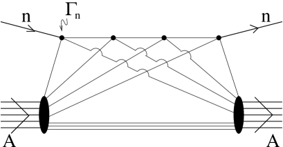
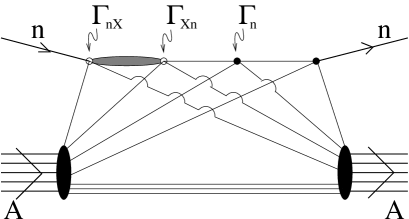
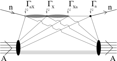
where , with , is the ground state wave function of the target nucleus, the impact parameter of the neutron moving along the -axis, and the nucleon-nucleon elastic profile function. The Inelastic Shadowing Profile should describe the diffractive dissociation of the neutron via the process and its de-excitation to the ground state by the process , as well as the elastic scattering of off the target nucleons. The three processes are described by the inelastic profiles and , and by the elastic profile , respectively. In our approach, as in Ref. [3], we will consider only two non-diagonal transitions, i.e. and , and the elastic scattering of . The corresponding diagrams are shown in Fig. 1. Within such an approximation, the Inelastic Shadowing profile can be written in the following form [3]:
| (4) | |||||
where
| (5) |
is the longitudinal momentum transfer. The basic nuclear ingredient appearing in Eqs. (3) and (4) is the square of the nuclear wave function , which can be written in terms of density matrices as follows [8]:
| (6) | |||||
in which is the one-body density matrix
| (7) |
and the two-body contraction is defined as follows:
| (8) |
where is the two-body density matrix
| (9) |
The one- and two-body density matrices appearing in Eq. (6) are normalized according to
| (10) |
and satisfy the following sequential conditions:
| (11) |
| (12) |
which leads to
| (13) |
In Eq. (6) only unlinked contractions have to be considered, and the higher order terms include unlinked products of 3, 4, etc. two-body contractions, unlinked products of three-body contractions, describing three-nucleon correlations, and so on. When all terms up to A-body correlations are written down explicitly, an identity is obtained.
The common approximation in Glauber type calculations consists in disregarding all terms of Eq. (6) but the first one. In this case the very well known expression for the total Glauber profile is given by
| (14) |
By taking into account two-body correlations, i.e. all unlinked products of two-body contractions in Eq. (6), one obtains [11, 12]
| (15) | |||||
which in the optical limit (A 1) becomes
| (16) |
As for the inelastic shadowing contribution (4), it can be reduced to an expression depending upon the total nucleon and diffractive cross sections and respectively.
| (17) | |||||
Within the approximation and disregarding correlations () the well-known Karmanov-Kondratyuk [13] expression is obtained
| (18) |
where depends upon .
In our calculations we have used both Eqs. (16) and (18). We have checked that the optical limit for is valid within , whereas correlations produce very tiny effects on . The ingredients of our calculations were as follows:
-
1.
The density matrices have been obtained by a linked cluster expansion for the one- and two-body density operators expectation value, evaluated over a fully-correlated wave function [9] obtained variationally with the Argonne interaction [10]. The one-body density has been obtained by integrating the two-body density. Let us stress that, unlike previous calculations, our two-body contractions (Eq. (8)) exactly satisfy the condition given by Eq. (13);
-
2.
the Glauber profile function is of the usual form
(19) with the energy-dependent parameters taken from [14];
-
3.
the parameters for the inelastic shadowing were taken from [6].
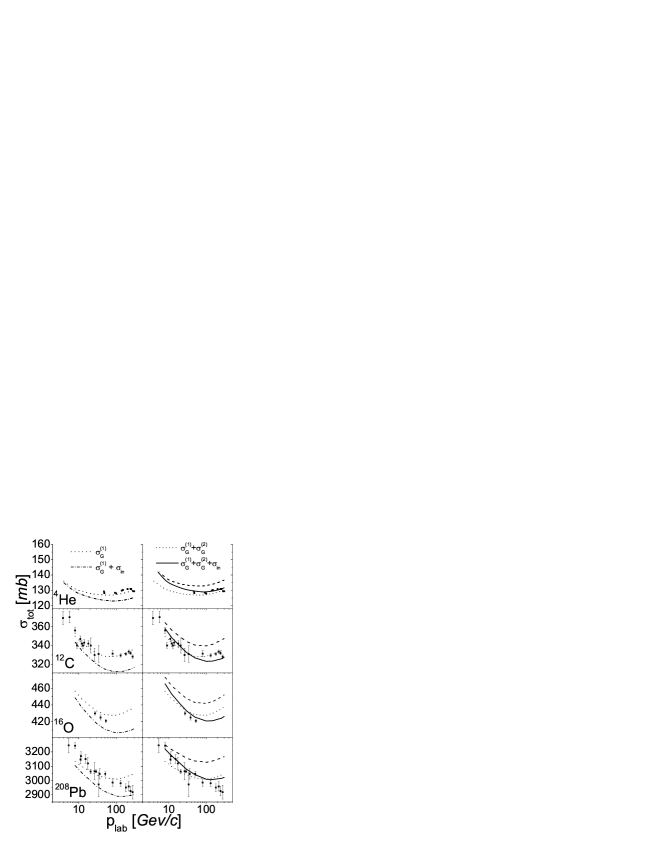
The results of calculations for , , and are presented in Fig. 2. The left panel shows the results obtained without correlations, whereas the effects of correlations are presented in the right panel. The results presented in Fig. 2 deserve the following comments:
-
1.
it can be seen that correlations increase the total cross section by about , i.e. they decrease the nuclear transparency, worsening the agreement with the experimental data when only Glauber shadowing is considered; the inclusion of inelastic shadowing brings back theoretical calculations in good agreement with experimental data;
-
2.
in the case of we have calculated the cross section to all orders of correlations using the exact wave function of Ref. [15]; it turns out that three- and four-nucleon correlations produce negligible effects on the total cross section;
-
3.
the effect of correlations is of the same order as the one from inelastic shadowing.
It should be pointed out that the contribution to the optical phase shift (the second term in the exponent of Eq. (16)) is always negative; the black disk limit of our approach is satisfied.
In Fig. 3 the difference between the two-body density calculated within the mean field, the cluster expansion and the following approximation for the two-body density
| (20) |
frequently used in case of complex nuclei (see e.g. Ref. [11]), is exhibited. The curves represent the quantity
| (21) |
It can be seen that the two-body density of Eq. (21) represents a poor representation of the realistic one. We have checked to what extent the sequential relation (13) is violated by the approximate two-body density matrix. The amount of violation of the integral in Eq. (13) can be checked by calculating the quantity
| (22) |
which is shown in Fig. 4 for various nuclei. Fig. 5 shows the effect of violation of the sequential relation on the total cross section.
2 A cluster expansion approach to the total cross section
We have developed a cluster-expansion [9] formulation for based upon the one-body distorted density matrix of Ref. [16], obtained taking into account two-nucleon correlations at first order of the cluster expansion and Glauber rescatterings at all orders. The zeroth-order approximation (i.e. with no correlation effects) is the same as Eq. (14); correlations can be included with the first term of the wave function expansion of Eq. (6), by replacing the one-body densities appearing in such a term with the distorted one-body density proposed in Ref. [16], in such a way one obtains contributions representing the interaction of the incident nucleon with the particles involved in each of the diagrams contributing to the distorted density (namely, the shell model, hole and spectator diagrams). The final expression for the total cross section reads as follows:
| (23) |
in which the shell model (), hole () and spectator contributions are as follows:
| (24) | |||||
Note that in the final calculations the shell model term has been exponentiated as in Eq. (16).
The results of calculations for obtained with Eq. (24) are compared in Fig. 5, with the results predicted, by Eqs. (6) and (20), respectively. It can be seen that the expansion based on the distorted density of Ref. [16] is in perfect agreement with the one of the approach based on the expansion of the wave function, Eq. (16), despite the different class of diagrams appearing in each contribution.
It should be stressed that the expansion used for the distorted one-body density can be used to calculate, as in Ref. [16], the total transparency in experiments and distorted momentum distributions, as in Refs. ([17, 18]) with the full correlated wave function for complex nuclei. Calculations of nuclear and color transparencies in and are in progress and will be reported elsewhere.
3 Summary and conclusions
We have developed a method which can be used to calculate scattering processes at medium and high energies within a realistic and parameter-free description of nuclear structure. Our calculations followed the following strategy:
-
i)
the values of the parameters pertaining to the correlation functions and the mean field wave functions, have been obtained from the calculation of the ground-state energy, radius and density of the nucleus using realistic nucleon-nucleon interactions;
-
ii)
using these parameters we have calculated the total neutron-Nucleus cross section taking rigorously into account two-nucleon correlations within the expansion of the exact wave function 6. We have also adopted a cluster expansion procedure [16] obtaining essentially the same results. This gives us confidence that the treatment of correlations is model independent to a large extent.
The method we have developed appears to be a very effective, transparent and parameter-free one and the main results we have obtained are:
-
i)
the effects generated by two-nucleon correlations (i.e. by those parts of the wave function expansion (6) which contain two-body contractions), are of the same order as Gribov inelastic shadowing; this, in our opinion, points to the necessity of an analysis of the accuracy of the common approximation used in medium-high energy hadronic scattering processes consisting in disregarding all terms of the expansion (6) but the first one;
-
ii)
correlations due to three and higher order contractions appear to produce only negligible effects on the total cross section.
4 Acknowledgements
We are indebted to Daniele Treleani, Boris Kopeliovich and Nikolai Nikolaev for many illuminating discussions.
References
- [1] R. J. Glauber, in Lectures in Theoretical Physics, W. E. Brittin et al Editors, New York (1959)
- [2] V. N. Gribov, Sov. JETP 29 (1969) 483; J. Pumplin, M. Ross, Phys. Rev. Lett. 21 (1968) 1778;
- [3] B. K. Jennings and G. A. Miller, Phys. Rev. C49 (1999) 2637.
- [4] B. Kopeliovich and J. Nemchik, Phys. Lett. B368 (1996) 187
- [5] B. Kopeliovich, Phys. Rev. C68 (2003) 044906
- [6] P. V. Murthy, C. A. Ayre, H.R. Gustafson, L. W. Jones and M. J. Longo, Nucl. Phys. B92, (1975) 269
- [7] N. N. Nikolaev, Sov. Phys. Usp. 24 (1981) 531
- [8] L. L. Foldy and J. D. Walecka, Ann. Phys. 54, (1969) 447
- [9] M. Alvioli, C. Ciofi degli Atti, H. Morita, Phys. Rev. C72 (2005) 054310
- [10] B. S. Pudliner, V. R. Pandharipande, J. Carlson, S. C. Pieper and R. B. Wiringa, Phys. Rev. C56, (1997) 1720
- [11] E. J. Moniz and G. D. Nixon, Ann. Phys. 67, (1971) 58
- [12] R. Guardiola and E. Oset, Nucl. Phys. A234 (1974) 458
- [13] V. A. Karmanov, L. A. Kondratyuk, JETP Lett. 18 (1973) 451
- [14] K. Hikasa, Particle Data Group Phys. Rev. D45 S1 (1992); M. M. Block, K. Kang and A. R. White, Int. J. Mod. Phys. A77 (1992) 4449
- [15] H. Morita, Y. Akaishi, O. Endo and H. Tanaka, Prog. Theor. Phys. 78 (1987) 1117
- [16] C. Ciofi degli Atti, D. Treleani, Phys. Rev. C60 (1999) 024602
- [17] M. Alvioli, C. Ciofi degli Atti, and H. Morita, Fizika B13 (2004) 585;
- [18] M. Alvioli, C. Ciofi degli Atti and H. Morita Int. J. Mod. Phys. B20 (2006) 5325
- [19] J. Engler et al., Phys. Lett. B32 (1970) 716; L. W. Jones et al., Phys. Lett. B36 (1971) 509
a)
b)
c)